Article

Drought Impacts on Vegetation in Southeastern Europe

by
Patrícia Páscoa
1,2,3,*,
Célia M. Gouveia
1,2,
Ana C. Russo
2,
Roxana Bojariu
4,
Sergio M. Vicente-Serrano
5 and
Ricardo M. Trigo
2,6
1
Instituto Português do Mar e da Atmosfera, 1749-077 Lisbon, Portugal
2
Instituto Dom Luiz, Faculdade de Ciências da Universidade de Lisboa, 1749-016 Lisbon, Portugal
3
Environmental Physics Laboratory (EPhysLab), Facultade de Ciencias, Universidad de Vigo, 32004 Ourense, Spain
4
National Meteorological Administration, 013686 Bucharest, Romania
5
Instituto Pirenaico de Ecología, (IPE-CSIC), 50192 Zaragoza, Spain
6
Departamento de Meteorologia, Universidade Federal do Rio de Janeiro, 21941-916 Rio de Janeiro, Brasil
*
Author to whom correspondence should be addressed.
Remote Sens. 2020, 12(13), 2156; https://doi.org/10.3390/rs12132156
Submission received: 25 May 2020 / Revised: 30 June 2020 / Accepted: 1 July 2020 / Published: 6 July 2020
(This article belongs to the Special Issue Feature Paper Special Issue on Forest Remote Sensing)

Abstract

:
We evaluated the response of vegetation’s photosynthetic activity to drought conditions from 1998 to 2014 over Romania and the Republic of Moldova. The connection between vegetation stress and drought events was assessed by means of a correlation analysis between the monthly Standardized Precipitation Evaporation Index (SPEI), at several time scales, and the Normalized Difference Vegetation Index (NDVI), as well as an assessment of the simultaneous occurrence of extremes in both indices. The analysis of the relationship between drought and vegetation was made for the growing season (from April to October of the entire period), and special attention was devoted to the severe drought event of 2000/2001, considered as the driest since 1961 for the study area. More than three quarters (77%) of the agricultural land exhibits a positive correlation between the two indices. The sensitivity of crop areas to drought is strong, as the impacts were detected from May to October, with a peak in July. On the other hand, forests were found to be less sensitive to drought, as the impacts were limited mostly to July and August. Moreover, vegetation of all land cover classes showed a dependence between the sign of the correlation and the elevation gradient. Roughly 60% (20%) of the study domain shows a concordance of anomalously low vegetation activity with dry conditions of at least 50% (80%) in August. By contrast, a lower value of concordance was observed over the Carpathian Mountains. During the severe drought event of 2000/2001, a decrease in vegetation activity was detected for most of the study area, showing a decrease lasting at least 4 months, between April and October, for more than two thirds (71%) of the study domain.

Graphical Abstract

1. Introduction

The destruction caused by natural disasters has significant economic, environmental and social impacts [1]. One of the most significant hydroclimatic hazards striking the environment and society is drought [2,3,4], but its effects are not easy to quantify, as the start, end, duration, intensity and spatial extent of a drought episode are not easy to determine [5]. Moreover, given the large number of environmental systems and socioeconomic sectors affected by drought, including agriculture [6,7], power production [8], water supply [9,10] and natural ecosystems [11,12,13], a simple and universal definition of drought is impossible [14]. Droughts are known to reduce the primary and secondary production of vegetation and forests [15,16], and to induce tree mortality episodes [17] and pasture loss [18]. However, the diverse resilience and resistance of many vegetation types to water scarcity [19,20,21,22], and the complex interactions between the severity and time scales of droughts with respect to their effects on vegetation [23,24,25], complicate the overall assessment of the impact of drought events on natural systems.
Several approaches to assessing the impact of drought on vegetation activity have been proposed, including: (i) analyses of the hydraulic properties of vegetation, on either a species or a biome level [26,27]; (ii) assessment of the impacts on tree growth based on tree-ring data [28,29]; (iii) analyses of crop yields [30,31]; (iv) phenological studies [32,33]; and v) monitoring vegetation using satellite data [34,35,36]. The latter approach is advantageous, since it allows repeated measurements with high spatial resolution to be made over large areas and at different times [37]. For example, the impacts of drought on vegetation activity and on crop yields have been evaluated using so-called vegetation indices, obtained from remote sensing information, such as the Normalized Differences Vegetation Index (NDVI), at local, regional or global scales [25,35,38,39,40,41,42,43].
Alternatively, meteorological variables can be used to compute multiscalar drought indicators, such as the Standardized Precipitation Index (SPI) [44] or the Standardized Precipitation Evapotranspiration Index (SPEI) [45], which can thus characterize drought impacts on different vegetation types and biomes. The advantage of using multiscalar drought indices is related to their ability to take differences in the response times of vegetations to water-deficit conditions into account [23,25,46,47], thereby facilitating determinations of the relationships between ecosystem variables and drought severity.
Southeastern Europe (SEE), a region located between the Mediterranean Sea and the Black Sea, encompassing Romania and the Republic of Moldova, is characterized by highly diverse bioclimatic features and vegetation types [48,49,50]. Intense land use over several centuries has altered the natural vegetation of SEE [51,52] in ways that are distinct from the anthropogenic changes in western Europe [53,54]. For example, agricultural intensification occurred later in SEE than in western Europe, and grasslands persisted in SEE for a longer period of time [55,56]. In addition, while between 1947 and 1989 the transfer to the state of land ownership led to the intensification of agriculture [57], after the regime change of 1989 this trend reversed, and large areas of farmland were abandoned [58,59]. In the forest regions, there are patches consisting of high percentages of monoculture plantations or semi-natural forests [60]. These areas are less resilient to climate variability than natural forests [61]. Nonetheless, there are also well-preserved natural ecosystems. In fact, the largest areas of pristine forests in eastern and central Europe are found in the Carpathian Mountains, and the biodiversity of those forests is very high [60]. Grasslands and agricultural mosaics in SEE also have a rich biodiversity [62], and provide habitats for several rare or endangered species, such as a number of species of butterfly [63]. Although the climate classification in Romania and the Republic of Moldova ranges from humid to dry [64], the annual water balance in areas mainly occupied by agriculture is negative, and becomes even more severe during the growing season [65].
Several relevant changes have recently been identified in the climate of SEE, such as increases in temperature [66,67] and in the atmospheric evaporative demand (AED) [68], that may alter the primary and secondary growth of many types of vegetation [69]. Climate change models predict increased climate-related impacts, including in SEE, where a decrease in precipitation during the warm season [70], but also an increase in the AED [64], are expected. The resulting increase in climate aridity, together with longer, more severe drought events, could have important effects on ecosystems in SEE. An in-depth evaluation of the responses of SEE biomes to drought events, which highlights the relation between vegetation activity and climate or environmental features such as topography, is therefore essential. This must include the impacts of severe drought events, which are known to cause short-term changes in productivity [71] but may also cause long-term impacts [17,72]. In this context, it is worth noticing that climate change scenarios for the region project an increase in the frequency and severity of these drought events at the end of the 21st century [73,74,75].
In this study, we analyzed the impacts of drought on vegetation activity in Romania and the Republic of Moldova using SPEI at several time scales and the satellite-derived NDVI. Our main objectives were: (i) to map the impact of drought conditions on vegetation activity; (ii) to analyze the response of the different land cover classes to drought; and (iii) to study the impact on vegetation activity of an extreme drought event.

2. Materials and Methods

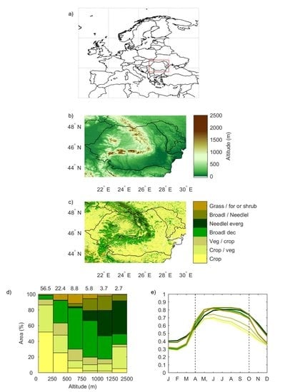
2.1. Land Cover and Elevation Data

The study area is located at 43°N–49˚N, 20.2˚E–30.1°E, as shown in Figure 1a. Land cover classification data with a spatial resolution of 300 m and containing 22 land cover classes were obtained from the Globcover 2009 project [76]. The majority rule and a nearest neighbor interpolation were used to resample the Globcover 2009 map to the resolution and coordinates of the NDVI data set used here (see Section 2.2). Urban areas, water bodies and land cover classes occupying a small area were discarded, so that only representative land cover classes were analyzed. The land cover classes that were not considered accounted only for < 1% of the study area. Elevation data were obtained from the GLOBE project [77] with a spatial resolution of 1 km, and were resampled to match the coordinates of the NDVI by means of a bilinear interpolation.
The area (%) of the land cover classes considered is shown in Table 1. Agricultural land occupied 70.6% of the area, and included the classes rainfed cropland (34.8%), and a mixture of cropland and natural vegetation (two classes occupying 26.2% and 9.6%, respectively). The three classes corresponding to forests occupy 23.7% of the area, and mixtures of grassland and forest/shrubland occupy 3.8%. Table 1 also lists the labels used in Figure 1, Figure 4, Figure 5 and Figure 7, and Table 4 and Table 5, to represent each of the land cover classes. Figure 1 also maps the elevation (b) and land cover classes (c). The distinct shape of the Carpathian Mountains (forested areas) is evident, as well as the elevation dependence of the land cover classes. Agricultural areas are the most common land cover classes at low elevations (Figure 1d), while at higher elevations, forests are more common, constituting the dominant land cover class at elevations higher than 500 m (Figure 1e). It is evident that forest classes change with elevation, the broadleaved forest being the more frequent land cover class at lower elevations and needleleaved forest, which account for only 3.3% of the total area, covering around 35% at elevations higher than 1000 m. It must be addressed that, even though in this mountainous region the elevation reached almost 2500 m, most of the study area (56.5%) was at an elevation below 250 m (Figure 1d).

2.2. Vegetation Index

Compared to in-situ methods, the data obtained via satellite allows large areas to be monitored at several spatial and temporal resolutions. Vegetation indices derived from remotely sensed data can be used to study vegetation status and variability. The NDVI is computed using reflectance measurements in the red and near-infrared channels; as a measure of vegetation greenness, the index is related to canopy structure, leaf area index and canopy photosynthesis [78,79].
The currently available NDVI datasets differ in their temporal and spatial resolutions, as well as the period they cover. The spatial resolution of the Global Inventory Modeling and Mapping Studies (GIMMS) dataset is 8 km and time series are available from the beginning of the 1980s, this being the longest available dataset covering the study area. Newer datasets have a higher spatial resolution, but encompass a shorter time period. An example is the NDVI dataset obtained using the SPOT VEGETATION instrument, available from 1998 to 2014, with a spatial resolution of 1 km, and the MODIS instrument, available since the beginning of the 21st century with a spatial resolution of 250 m. Taking into account the extent of the study area and the previous experience of using the SPOT VEGETATION dataset in similar assessments of vegetation dynamics and drought at a regional scale [34,36,80], the SPOT/VGT Collection 3 [81] was considered to be the most appropriate for our study. The SPOT/VGT Collection 3 dataset provided a value for every 10 days and covers the period from April 1998 to May 2014. The data was computed using atmospherically corrected and geometrically calibrated data, and was retrieved using the maximum value composite technique [82]. In our study, pixels identified as snow cover by the status map (information included in the dataset, at pixel basis, regarding the presence of clouds, cloud shadows or ice) were excluded, as were NDVI values < 0.1, because they do not represent vegetation.
Monthly NDVI time series were built by choosing the highest NDVI value on a monthly basis, and the median monthly values were computed for each land cover class, as shown in Figure 1e. While in the winter months vegetation activity was lower on all land cover classes, although increasing significantly in April and May, the highest NDVI value was reached in June for almost all land cover classes. The exception was needleleaved forests, where the NDVI was highest in August. In November, the NDVI values decreased abruptly. The present assessment was performed in the months from April to October, as they correspond to the months with the highest NDVI values, wherein it is expected to identify the highest signal of drought variability [42]. This period agrees with the start and end of the growing season in the study area, as obtained with experimental data [83].

2.3. Drought Index

Drought indices have been widely used to identify the occurrence of drought events, as well as their duration, intensity and spatial extent [84]. Because the impacts of droughts manifest at different time scales, potentially accumulating over time and lasting months or even years after the drought event has ended, they are best evaluated using a multiscalar drought index [84]. The multiscalar drought index SPI is computed using only precipitation data [44], and the SPEI requires a simple water balance, computed as the difference between precipitation and the AED [45]. The time scale corresponds to the number of months used to accumulate precipitation, in the case of SPI, and water-deficit, in the case of SPEI. The use of the AED is particularly suitable to evaluating the influence of drought conditions, and their variability, on vegetation activity [23,25,31,45,85,86,87]. Because the SPEI is standardized, it can be computed for all regions and compared directly, regardless of the climatology.
Therefore, in this study SPEI was used to assess drought conditions and their variability. The precipitation and AED data used to compute the SPEI were obtained from the Climate Research Unit (CRU) TS3.23 database. This database provides potential evapotranspiration, computed on a monthly time scale using a variant of the Penman–Monteith method [88]. This variable is a metric of the AED and was therefore used in this work. The data have a 0.5° spatial resolution and cover the period between 1901 and 2014 [88]. SPEI was computed for 5 different times scales (1-, 3-, 6-, 9- and 12-month), in order to reflect the different responses of the several land cover classes, as was done previously for the entire Mediterranean basin [25]. The classification of drought severity used in this work was that proposed by Agnew [89], and is shown in Table 2, together with the return period of each class. Considering the return periods of different droughts, the threshold of −0.84 was chosen to identify drought events. This threshold corresponds to the most severe drought event expected over a 5-year period [89].

2.4. Analysis

2.4.1. Correlation Analysis

This analysis followed an approach similar to the one adopted by Gouveia et al. [25], in which the response of vegetation to drought episodes over the Mediterranean basin was evaluated using the NDVI from the GIMMS dataset, at an 8-km spatial resolution, and SPEI. A correlation analysis between the monthly NDVI values and SPEI for the 5 selected timescales was performed, using the two-tailed Pearson correlation coefficient and considering a level of significance of 0.1. To avoid erroneous interpretations of correlation values, affected by the existence of trends in the time series related with changes in drought occurrence and severity [90,91], advances in agricultural technologies [92,93] and/or CO2 fertilization [94,95], both monthly time series NDVI and SPEI were previously detrended. Moreover, a bilinear interpolation was used to resample the SPEI time series so that it matched the resolution of the NDVI. Considering the relatively low spatial variability of the drought phenomena, and also the low temporal resolution used in this work, the interpolation performed is not expected to significantly change the variability of the SPEI time series [96], and thus should not significantly impact the correlation coefficients obtained.
To evaluate the drought’s influence on the different land cover classes, the percentage of area showing significant correlations, positive or negative, was computed for the 5 considered SPEI time scales. The mean and standard deviation of the significant correlation values obtained, considering each land cover class, time scale and month, were also obtained. It should be noted that the occurrence of a land cover class depends on elevation, which may also have influenced the results (Figure 1d). Consequently, for the months of June and July, the percent area with significant correlations was computed at several elevation intervals.

2.4.2. Occurrence of Vegetation Stress and Drought

The interannual variability of the climate conditions is reflected in the obtained correlation values between the SPEI and NDVI, including the influence of dry and wet episodes, and all severity classes. In order to evaluate in more detail the effects of dry conditions, the simultaneous occurrence of vegetation stress and drought conditions was assessed. As demonstrated in a number of studies conducted in different regions of the globe, vegetation stress is reflected by persistent negative NDVI anomalies (e.g., [34,36,80]). Monthly NDVI anomalies were obtained by subtracting the NDVI values from the monthly median. Sensitivity tests were performed to choose the threshold of NDVI anomalies that adequately identified the vegetation under stress conditions. Taking into account the land cover classes, vegetation was classified as being under stress if the NDVI anomaly was lower than −0.025 (NDVIanom25). This threshold was successfully used in a previous study of a region with similar vegetation types [34,35]. The simultaneous occurrence of NDVIanom25 and SPEI values lower than −0.84 (SPEI84, Table 2) was then computed, as a percentage of the total number of SPEI84, for each month and time scale, over the entire period.

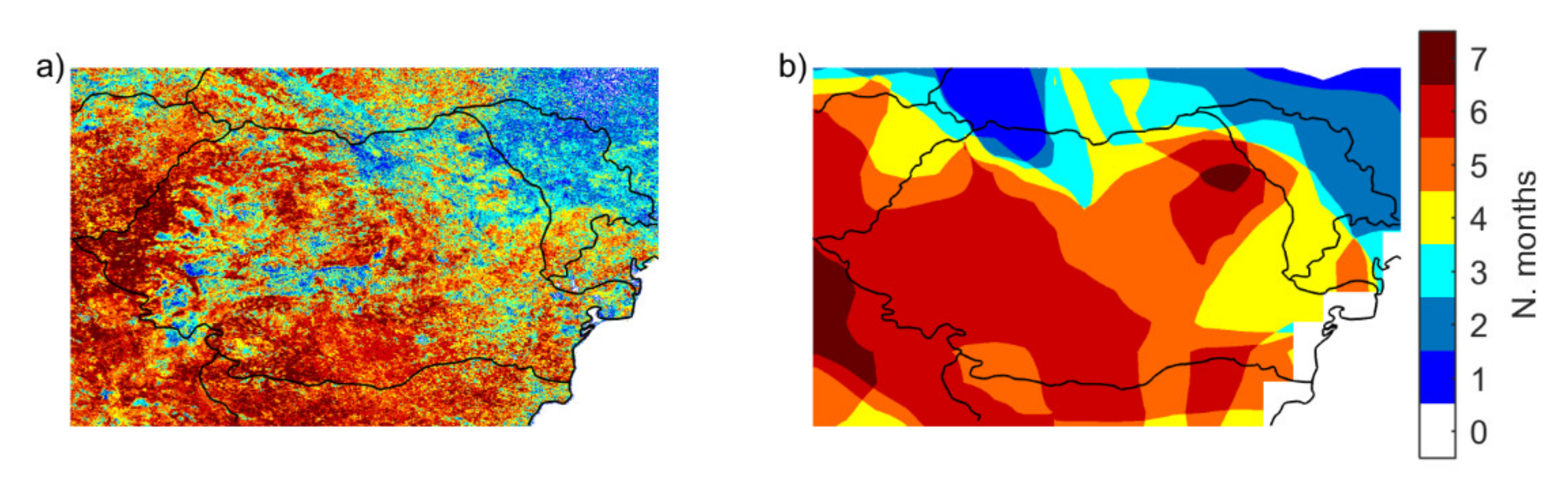
2.4.3. Drought Event of 2000/2001

The study area has been affected by several drought events in the last few decades. During the studied period (1998–2014), drought events were identified in 2000, 2002, 2003, 2007 and 2011 [97,98]. The drought event in 2000/2001 was considered the most severe drought during the period 1960–2013 [97,98], not only due to its intensity, but also to its duration. Spinoni et al. (2013) [97] identified June 2000 as the start, and February 2001 as the end of this drought event, using the SPI and SPEI at a 6-month time scale. The impact of the drought was particularly evident in Romania, Hungary and Bulgaria [99], Greece, Turkey, Italy, and the Balkan countries [100], and included reduced crop yields [99] and hydroelectrical production [101]. These authors point to an affected area of 30–40% in these regions, while in Romania it reached 60% [98], which resulted in an estimated economical cost of USD 500 million (EM-DAT, International Disaster Database, in [99]).
We applied the approach proposed by Gouveia et al. [34] to assess the effects on vegetation of this extreme drought event. Only the drought-affected months in 2000 were considered, since in 2001 the drought occurred before the start of the growing season [97]. Therefore, the persistence of NDVIanom25 was computed, on a pixel-level, by summing the number of months (from April to October 2000) that presented NDVI anomalies lower than −0.025. This methodology was also applied for SPEI84. Finally, we mapped the land cover classes for the regions presenting drought duration periods longer than 2 months, as identified by SPEI 6. The mapping was performed for both the shorter (less than 5 months) and longer (5 months or more) persistence of NDVIanom25.

3. Results

3.1. Spatial Distribution of Vegetation Response to drought Conditions

3.1.1. Correlation between SPEI and NDVI

Figure 2 maps the monthly correlation between the SPEI at 1-, 3- and 6-month time scales and the NDVI during the months from April to October. The results obtained using the time scales of 9 and 12 months were excluded from the analysis, as they were very similar to those obtained at 6 months. Negative correlations between the NDVI and SPEI were more frequent in May and June, mostly for the Carpathians, though positive correlations during these months were noted as well (Figure 2). In June, most of the correlations between the NDVI and SPEI were positive in the extra-Carpathian regions, and the areas in which this was the case increased in size as the time scale increased. No significant correlations at shorter time scales were found in the area south of the Carpathians in June. In July and August, at a 3-month time scale, a pattern of positive significant correlation is evident over this area, whereas in the Carpathian Mountains and the areas to the north the correlation values were less significant (Figure 2).

3.1.2. Occurrence of Vegetation Stress and Drought

The impacts of dry conditions on NDVI were additionally evaluated by counting the number of months in which both NDVI and SPEI anomalies were extremely negative. The obtained results are shown as a percentage relative to the number of SPEI84, and the areas with at least 50% and 80% (Table 3) concordance for each time scale and month were also computed. The spatial patterns of the simultaneous occurrence of NDVIanom25 and SPEI84 presented a dependence on both the analyzed month and the time scale for both the SPEI, and exhibited spatial variability (Figure 3). Simultaneous occurrence of SPEI84 and NDVIanom25 occurred in May in the central region, in June in the northeast and in July in the south (Figure 3). The results obtained for August are similar to those obtained for July. At the shortest time scale, the area showing a concordance of SPEI84 and NDVIanom25 of at least 50% was higher in May, and it increased from June to October, as well as with the time scale. A concordance of at least 80% was reached in a small area, with a peak in May, and in larger areas in September and October. The Carpathians had a lower concordance than the other areas, consistent with the negative correlations found in this area.

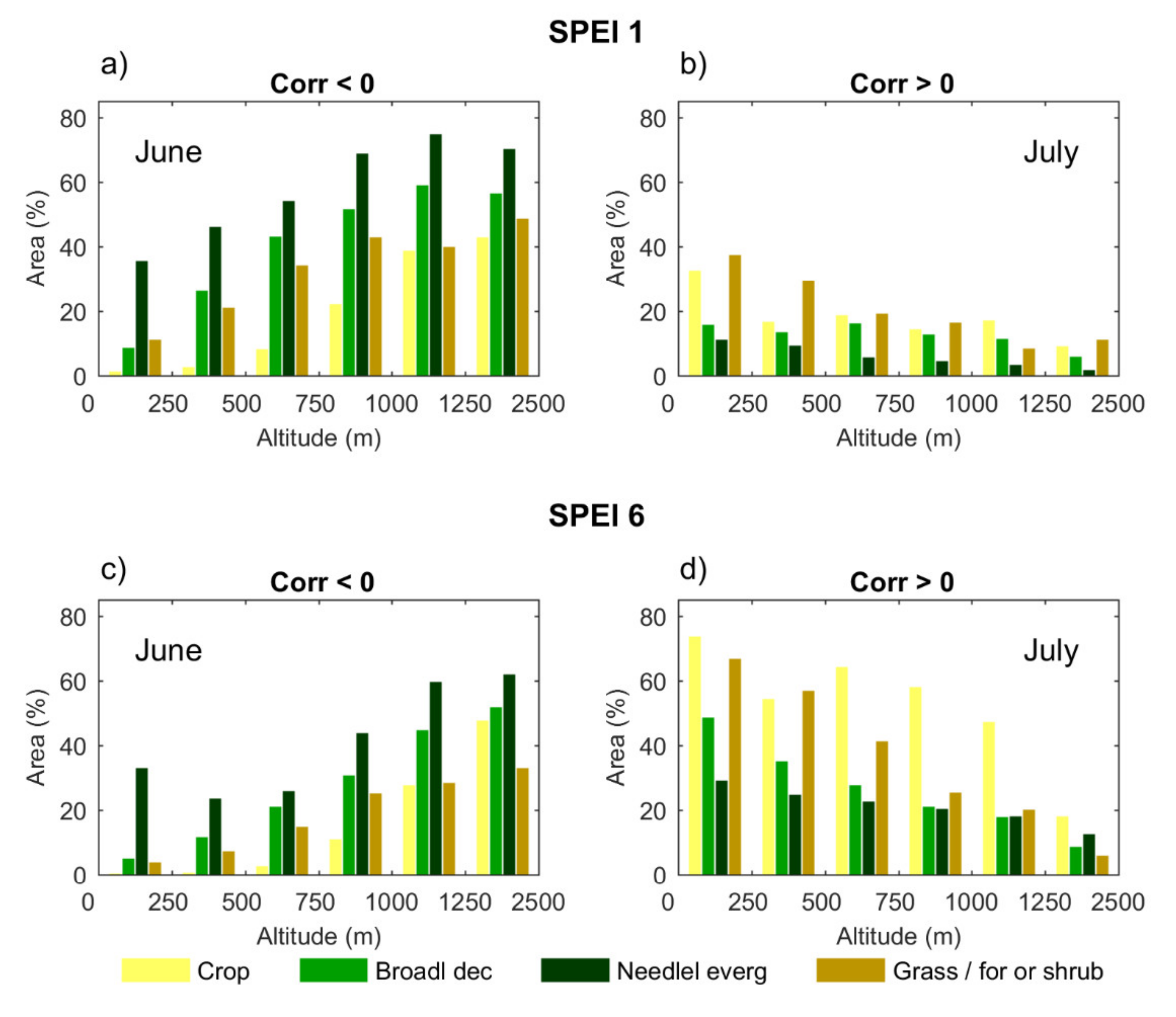
3.2. Response of Land Cover Classes to Drought Conditions

The areas (%) characterized by significant positive and negative correlations for each land cover class are shown in Table 4 and Table 5, respectively. Agricultural land is the land cover class showing the largest areas with positive correlation values from April to June (Table 4). Specifically, the areas showing significant positive correlations increased with the SPEI time scale and over time, exceeding one third (37%) of the total cropland area in June. From July onwards, the surface area (%) presenting positive correlations, considering the 6-month SPEI time scale, was very high (Table 4): more than three quarters (76%) of the cropland in August, and two thirds (65%) of the grassland in September. Similarly, for broadleaved forests, areas with positive correlations were particularly large during July, August, and September, with a maximum in August (42%) at a 6-month time scale. Considering needleleaved forests, the area (%) with a significant positive correlation was much lower, reaching only 17% in July (at a 6-month time scale) and even lower values in the other months (Table 4). As expected from Figure 2, the largest areas of negative correlations occurred in May and June (Table 5). Negative correlation values obtained for the time scale of 1-month were more frequent in June for needleleaved (70%) and broadleaved (35%) forests, followed by a mixture of grassland and forest or shrubland (25%). In the case of the mixture of broadleaved and needleleaved forests, the affected area is similar to the one observed for needleleaved forests.
Correlations are strongly related to the elevation. Figure 4 shows the area (%) presenting significant correlation values for different land covers classes: cropland, broadleaved forest, needleleaved forest and grassland, considering several elevation intervals, and the time scales of 1 month [a) and b)] and 6 months [c) and d)]. Only the positive correlations obtained in June and the negative correlations obtained in July are shown and analyzed. Negative (positive) correlations were mainly observed at higher (lower) elevations, and a reduction of the size of the area was obtained with decreasing (increasing) elevation. The largest (smallest) area of negative (positive) correlations was observed for needleleaved forests at all the elevation intervals. Furthermore, a large area of positive correlations was observed for cropland. Moreover, with the exception of SPEI 6 for croplands, the grassland cover class accounted for the largest area of positive correlations at almost all intervals.
Figure 5 depicts, for each land cover class, the mean values of the significant correlations and corresponding standard deviations (only values lower than 0.2 are shown) obtained for each time scale and month. In agricultural areas, the mean correlation was mostly positive, but the standard deviation was low only from July onwards. For land cover consisting of forest, the area of significant correlations was smaller, but there was a clear pattern of negative correlations between April and June, and of positive correlations starting in July. Nonetheless, the mean correlation values for needleleaved forests were again negative (often significantly) in August and later when considered at short time scales.
The contrasting patterns of correlations obtained for forests and croplands are consistent with the different seasonal cycles of these land cover classes. It must be stressed that the high NDVI values observed over needleleaved forests (including mixed broadleaved and needleleaved forest) were maintained until October (Figure 1e), whereas in the remaining land cover classes, greenness started to decrease in June. Nonetheless, grasslands, as well as needleleaved and broadleaved forests, exhibited high NDVI values between June and October. The correlation patterns for these land cover classes were very similar (Figure 5), although presenting contrasting patterns of standard deviation. Needleleaved forests presented the lowest values of standard deviation until June, whereas the values obtained for broadleaved forests and grasslands were lowest after July, reflecting the different areas presented in Table 4 and Table 5. This feature also highlights the greater sensitivity of needleleaved forests, in the case of negative correlations, contrasting with the opposite sign of response to drought in the case of broadleaved forests.

3.3. Impact of the Drought Event of 2000/2001

In this section we evaluated the impact of the 2000/2001 drought episode. Our assessment is based on an in-depth analysis of the NDVI anomalies from April to October 2000, which corresponds to the growing season during the drought event. The number of months displaying NDVIanom25 and SPEI84 are shown in Figure 6a,b, respectively. The northeastern region and part of the Carpathians were less affected by the drought, as evidenced by the persistence of low NDVI anomalies for 3 months or less (Figure 6a). In the remaining region, NDVIanom25 occurred for at least 4 months in roughly 70% of the area, and for at least 5 months in approximately 50% of the area. Moreover, drought conditions, as obtained by SPEI, are spread over most of the study area (Figure 6b). The main spatial pattern of reduction in the vegetation activity, as obtained through NDVI anomalies, was generally in accordance with the spatial pattern of SPEI, thus identifying that this drought event is linked with the decreased vegetation activity. According to SPEI, dry conditions persisted for a shorter time in the north and northeast, which explained the NDVI results. However, the spatial pattern for the Carpathian Mountains differed from the ones in the remaining areas.
An additional assessment was made for the regions where drought duration was longer than 2 months (Figure 6b), by analyzing separately the land cover classes showing a persistence of NDVIanom25 of less than 5 months (Figure 7a) and 5 months or more (Figure 7b). Figure 6b shows that a link between the persistence of low NDVI anomalies and the duration of the drought is evident for agricultural land cover classes. The needleleaved forests were the least affected, with NDVIanom25 persisting for less than 5 months in most of its areas (Figure 7b). This is likely related to the fact that this land cover class appears primarily at high elevations. Conversely, broadleaved forests appear mostly at lower elevations, where the persistence of NDVIanom25 in this land cover class is longer (Figure 7b) than it is at high elevations (Figure 7a). Nonetheless, it should be highlighted that the northern area showed less severe drought conditions than in the south, and consequently a lower impact on vegetation is to be expected (Figure 7a).

4. Discussion

Here we have analyzed the impact of drought severity on vegetation activity in SEE, considering not only distinct time lags but also different land cover classes and elevation ranges. Additionally, we have analyzed the conditions under the most extreme drought event recorded in the last five decades.
The correlations between SPEI and NDVI agree with previous works done in the study area. Potopová et al. (2016) [102] examined drought effects on several crops in Moldova, and found them to be lower in April and higher from July onwards. Levanič et al. (2013) [103] examined the relationship between monthly precipitation and Pinus nigra tree-ring widths in southern Romania, and found that the correlation was also strongest in July; however, when using the 3-month SPI, the correlation was strongest in July, August and September. The correlation values between SPEI and NDVI reflect the water balance, and have a tendency to increase when the latter decreases [23,25]. In our study area, monthly mean precipitation is highest in June [104,105,106], whereas the maximum monthly temperature occurs in July [106,107]. Therefore, it is possible to associate the decrease in soil water content with the increase of the values of correlation between NDVI and SPEI. The correlations were mainly negative (positive) at high (low) elevations, which is in agreement with the fact that the factors limiting vegetation photosynthetic activity are dependent on elevation, as a response to the varying climate conditions observed. Moreover, photosynthetic activity is more likely to be limited by radiation and/or temperature in humid and cold mountainous regions [108]. Gouveia et al. (2017) [25] found similar patterns of negative and positive correlations, although the negative correlations presented by those authors were not significant, since they analyzed fewer months. The negative correlations, at high elevations, obtained here occurred during the months when both the NDVI values and the precipitation levels were higher, similar to the results previously reported for this area [109], pointing to temperature or radiation as the main factors controlling vegetation activity. Sidor et al. (2015) [110] analyzed the tree-rings of Norway spruce stands in the eastern Carpathian Mountains, and found a positive effect of temperature at high elevations, as well as a negative influence of precipitation in June and July, demonstrating that temperature is not the sole driver of vegetation activity at high elevations. Nonetheless, precipitation is inversely related to radiation, therefore both the correlation identified by Sidor et al. (2015) [110] and our own results can be explained accordingly. Specifically, a decrease in precipitation may imply an increase of cloud free sky, and thus radiation, which limits vegetation activity. At lower elevations, the relationship between tree growth and precipitation/temperature is inverted, and the authors suggest that water stress may induce negative responses to temperature [110]. Our results showed a subsequent sign change in July, which may be associated with the combined effect of increasing temperature and decreasing precipitation (and thus water stress). At shorter time scales, and contrasting with low elevation regions, the correlation values at high elevations were mostly non-significant, coinciding with the higher values of water balance. Nonetheless, the size of the area (%) in which the correlation was positive also increased with longer time scales, indicative of the impacts on the vegetation of longer periods of lower water balance, despite the humid climate at high elevations. The effect was likely exacerbated by the increased vegetation activity in June, which may result in soil water depletion, and by the decreased water availability during the driest months.
Low values of NDVI anomalies indicate the potentially negative impact of drought episodes on vegetation activity occurring in areas where the correlation is negative or non-significant. This feature has previously been shown in the Iberian Peninsula, where some regions showing non-significant correlations between wheat yield and SPEI also showed a high simultaneous occurrence of low wheat yield anomalies and drought conditions [31,111]. Although a simultaneous occurrence of SPEI84 and NDVIanom25 was observed in over half of the study area, the small area of significant correlations during April and May suggested that drought conditions had little influence on vegetation activity.
Among the studied land cover classes, the most sensitive to drought was agricultural land, as cropland displayed a larger area of significant positive correlation values, and a much smaller area of negative correlations. Similar results were obtained by Schwalm et al. [112] through the application of a different approach based on the use of FLUXNET data, which showed a negative impact of droughts on the productivity of croplands. For agricultural land (and grasslands from June onwards), positive correlations were relatively high even at smaller time scales (1- and 3-month), which indicates a strong reaction even to brief drought periods. The importance of summer months (July onwards) for the agricultural land, grassland and broadleaved forest land cover classes is highlighted by the obtained low standard deviations. However, although positive correlations were also determined for needleleaved and mixed forests throughout the summer months, the smaller area with significant positive correlation values, and the large standard deviations, implied that these land cover classes were less susceptible to drought. A dual behavior was identified for all land cover classes, as for the month of June (July), negative (positive) correlations were determined, and the size of the affected area increased (decreased) with increasing elevation. These results are in accordance with those reported by Sidor et al. [110] for the Carpathians, and for lower-elevation areas by Baumbach et al. [113].
The impact of the 2000/2001 drought event was consistent with the different climate-related limitations to vegetation activity within the respective elevation range [108,114]. The negative correlations of NDVI and SPEI, coupled with the low concordance of the negative NDVI anomalies and negative SPEI values (Figure 3), were consistent with vegetation stress of shorter duration in the Carpathians during this severe drought event. The drought episode of 2000/01 was equivalent in severity to that of other drought events that occurred in Europe, such as the pan-European drought in 2003 and the drought in the Iberian Peninsula in 2005. The impacts of both these latter events on vegetation and net primary production have been assessed [35,71], but the impact of the drought event of 2000/01 has received little interest. A distinct reaction from vegetation was identified in the study area, which reflected its varying responses and high geographic diversity, contrarily to the usual homogeneous response of vegetation in low-diversity regions.
Furthermore, our results showed that strong drought episodes have a significant impact, even on humid areas, since low NDVI anomalies occurred even at higher elevations, which implies that humid vegetation communities have a differentiated response to different levels of drought and are very sensitive to extreme drought episodes, due to their low ecophysiological resistance to water deficits [19,20].

5. Conclusions

The impacts of droughts on vegetation in SEE were analyzed through the application of a multi-scale drought indicator (SPEI) and a vegetation index (NDVI). The proposed approach, applied to the growing season of vegetation (April to October), allowed the identification of spatial patterns of drought-dependence in the most common land cover classes of the study area, namely three classes of croplands and of forest, and grasslands.
Significant correlations were detected across most of the study area, which were dominated by varied spatial patterns according to the growing state of the vegetation. The main findings of this study can be summarized as follows:
(i)
during the first months of the growing season (April to June), areas with significant correlation values (both positive and negative) increased at all time scales;
(ii)
the middle period of the growing season (July and August) showed almost only positive correlations at all time scales;
(iii)
finally, positive correlations start disappearing from September onwards, starting at shorter time scales.
Another aspect that was identified in the present study was the relation to elevation, which was indicated by the general association of high (low) elevation with the presence of negative (positive) correlations between the NDVI and SPEI. In order to complement the correlation analysis, we analysed the simultaneous occurrence of both negative NDVI anomalies and SPEI values. The results reinforced some of the findings of the former, in that areas with a higher (lower) concordance generally coincided with areas of positive (negative) correlations.
The high response to drought of agricultural land during the entire growing season, contrary to what is seen for needleleaved forests, was observable through the application of separate analyses for the different land cover classes in the region. Indeed, grasslands and forests showed a lower response to drought conditions, particularly from July onwards, but this response is however dependent on elevation.
Finally, the spatial mapping of the impacts of the major registered drought event in the study area during the growing season of 2000 showed decreased vegetation activity across the entire study area, in accordance with the drought conditions assessed by SPEI. The duration of this negative impact was similar to that identified in the correlation and concordance analysis. Thus, the drought, while severe, was of shorter duration in the Carpathian Mountains than in the other areas of the study location. In addition, the decrease of vegetation activity in needleleaved forests, which were shown to be of low drought sensitivity, was of shorter duration than that seen in highly sensitive agricultural land and grasslands.

Author Contributions

Conceptualization, P.P., C.M.G., A.C.R., R.B., S.M.V.-S. and R.M.T.; Data curation, P.P. and A.C.R.; Formal analysis, P.P.; Funding acquisition, C.M.G., R.B., S.M.V.-S. and R.M.T.; Investigation, P.P. and A.C.R.; Methodology, P.P. and C.M.G.; Writing—original draft, P.P.; Writing–review and editing, C.M.G., A.C.R., R.B., S.V.-S. and R.M.T. All authors have read and agreed to the published version of the manuscript.

Funding

This work was partially supported by national funds through FCT (Fundacão para a Ciência e a Tecnologia, Portugal) under Project IMDROFLOOD (WaterJPI/0004/2014) and the research grant attributed to Ana Russo (SFRH/BPD/99757/2014). One of the authors also acknowledge the support of the Romanian Executive Unit for Financing Higher Education, Research, Development and Innovation (UEFISCDI) under Grant no. 81/2016.

Conflicts of Interest

The authors declare no conflict of interest.

References

  1. Kelman, I.; Gaillard, J.; Lewis, J.; Mercer, J. Learning from the history of disaster vulnerability and resilience research and practice for climate change. Nat. Hazards 2016, 82, 129–143. [Google Scholar] [CrossRef] [Green Version]
  2. Below, R.; Grover-Kopec, E.; Dilley, M. Documenting Drought-Related Disasters: A Global Reassessment. J. Environ. Dev. 2007, 16, 328–344. [Google Scholar] [CrossRef]
  3. Carrão, H.; Naumann, G.; Barbosa, P. Mapping global patterns of drought risk: An empirical framework based on sub-national estimates of hazard, exposure and vulnerability. Glob. Environ. Chang. 2016, 39, 108–124. [Google Scholar] [CrossRef]
  4. Wilhite, D.A.; Pulwarty, R.S. Drought as a hazard: Understanding the natural and the social context. In Drought and Water Crisis. Integrating Science, Management, and Policy; CRC Press: Boca Raton, FL, USA, 2017; pp. 3–20. [Google Scholar]
  5. Wilhite, D.A. Drought as a natural hazard: Concepts and definitions. In Drought: A Global Assessment; Routledge: New York, NY, USA, 2000; Volume 1, pp. 3–18. [Google Scholar]
  6. Li, Y.; Ye, W.; Wang, M.; Yan, X. Climate change and drought: A risk assessment of crop-yield impacts. Clim. Res. 2009, 39, 31–46. [Google Scholar] [CrossRef]
  7. Lesk, C.; Rowhani, P.; Ramankutty, N. Influence of extreme weather disasters on global crop production. Nature 2016, 529, 84–87. [Google Scholar] [CrossRef] [PubMed]
  8. Stagge, J.H.; Kohn, I.; Tallaksen, L.M.; Stahl, K. Modeling drought impact occurrence based on meteorological drought indices in Europe. J. Hydrol. 2015, 530, 37–50. [Google Scholar] [CrossRef]
  9. De Wit, M.; Stankiewicz, J. Changes in Surface Water Supply Across Africa with Predicted Climate Change. Science 2006, 311, 1917. [Google Scholar] [CrossRef] [Green Version]
  10. Rajagopalan, B.; Nowak, K.; Prairie, J.; Hoerling, M.; Harding, B.; Barsugli, J.; Ray, A.; Udall, B. Water supply risk on the Colorado River: Can management mitigate? Water Resour. Res. 2009, 45. [Google Scholar] [CrossRef]
  11. Allen, C.D.; Breshears, D.D. Drought-induced shift of a forest–woodland ecotone: Rapid landscape response to climate variation. Proc. Natl. Acad. Sci. USA 1998, 95, 14839. [Google Scholar] [CrossRef] [Green Version]
  12. Zeng, N.; Qian, H.; Roedenbeck, C.; Heimann, M. Impact of 1998–2002 midlatitude drought and warming on terrestrial ecosystem and the global carbon cycle. Geophys. Res. Lett. 2005, 32. [Google Scholar] [CrossRef] [Green Version]
  13. Fauset, S.; Baker, T.R.; Lewis, S.L.; Feldpausch, T.R.; Affum-Baffoe, K.; Foli, E.G.; Hamer, K.C.; Swaine, M.D. Drought-induced shifts in the floristic and functional composition of tropical forests in Ghana. Ecol. Lett. 2012, 15, 1120–1129. [Google Scholar] [CrossRef]
  14. Lloyd-Hughes, B. The impracticality of a universal drought definition. Theor. Appl. Climatol. 2014, 117, 607–611. [Google Scholar] [CrossRef] [Green Version]
  15. Martínez-Alonso, C.; Valladares, F.; Camarero, J.J.; Arias, M.L.; Serrano, M.; Rodríguez, J.A. The uncoupling of secondary growth, cone and litter production by intradecadal climatic variability in a mediterranean scots pine forest. For. Ecol. Manag. 2007, 253, 19–29. [Google Scholar] [CrossRef]
  16. Bennett, A.C.; McDowell, N.G.; Allen, C.D.; Anderson-Teixeira, K.J. Larger trees suffer most during drought in forests worldwide. Nat. Plants 2015, 1, 15139. [Google Scholar] [CrossRef] [PubMed]
  17. Allen, C.D.; Macalady, A.K.; Chenchouni, H.; Bachelet, D.; McDowell, N.; Vennetier, M.; Kitzberger, T.; Rigling, A.; Breshears, D.D.; Hogg, E.T.; et al. A global overview of drought and heat-induced tree mortality reveals emerging climate change risks for forests. For. Ecol. Manag. 2010, 259, 660–684. [Google Scholar] [CrossRef] [Green Version]
  18. Smit, H.J.; Metzger, M.J.; Ewert, F. Spatial distribution of grassland productivity and land use in Europe. Agric. Syst. 2008, 98, 208–219. [Google Scholar] [CrossRef]
  19. Chaves, M.M.; Maroco, J.P.; Pereira, J.S. Understanding plant responses to drought—From genes to the whole plant. Funct. Plant Biol. 2003, 30, 239–264. [Google Scholar] [CrossRef]
  20. McDowell, N.; Pockman, W.T.; Allen, C.D.; Breshears, D.D.; Cobb, N.; Kolb, T.; Plaut, J.; Sperry, J.; West, A.; Williams, D.G.; et al. Mechanisms of plant survival and mortality during drought: Why do some plants survive while others succumb to drought? New Phytol. 2008, 178, 719–739. [Google Scholar] [CrossRef] [PubMed]
  21. Gazol, A.; Camarero, J.J.; Vicente-Serrano, S.M.; Sánchez-Salguero, R.; Gutiérrez, E.; de Luis, M.; Sangüesa-Barreda, G.; Novak, K.; Rozas, V.; Tíscar, P.A.; et al. Forest resilience to drought varies across biomes. Glob. Chang. Biol. 2018, 24, 2143–2158. [Google Scholar] [CrossRef]
  22. Kannenberg, S.A.; Schwalm, C.R.; Anderegg, W.R.L. Ghosts of the past: How drought legacy effects shape forest functioning and carbon cycling. Ecol. Lett. 2020, 23, 891–901. [Google Scholar] [CrossRef] [Green Version]
  23. Vicente-Serrano, S.M.; Gouveia, C.; Camarero, J.J.; Beguería, S.; Trigo, R.; López-Moreno, J.I.; Azorín-Molina, C.; Pasho, E.; Lorenzo-Lacruz, J.; Revuelto, J.; et al. Response of vegetation to drought time-scales across global land biomes. Proc. Natl. Acad. Sci. USA 2013, 110, 52. [Google Scholar] [CrossRef] [PubMed] [Green Version]
  24. Vicente-Serrano, S.M.; Camarero, J.J.; Azorin-Molina, C. Diverse responses of forest growth to drought time-scales in the Northern Hemisphere. Glob. Ecol. Biogeogr. 2014, 23, 1019–1030. [Google Scholar] [CrossRef] [Green Version]
  25. Gouveia, C.M.; Trigo, R.M.; Beguería, S.; Vicente-Serrano, S.M. Drought impacts on vegetation activity in the Mediterranean region: An assessment using remote sensing data and multi-scale drought indicators. Glob. Planet. Chang. 2017, 151, 15–27. [Google Scholar] [CrossRef] [Green Version]
  26. Anderegg, W.R.; Berry, J.A.; Smith, D.D.; Sperry, J.S.; Anderegg, L.D.; Field, C.B. The roles of hydraulic and carbon stress in a widespread climate-induced forest die-off. Proc. Natl. Acad. Sci. USA 2012, 109, 233–237. [Google Scholar] [CrossRef] [PubMed] [Green Version]
  27. Choat, B.; Jansen, S.; Brodribb, T.J.; Cochard, H.; Delzon, S.; Bhaskar, R.; Bucci, S.J.; Feild, T.S.; Gleason, S.M.; Hacke, U.G.; et al. Global convergence in the vulnerability of forests to drought. Nature 2012, 491, 752–755. [Google Scholar] [CrossRef] [Green Version]
  28. Rigling, A.; Bräker, O.; Schneiter, G.; Schweingruber, F. Intra-annual tree-ring parameters indicating differences in drought stress of Pinus sylvestris forests within the Erico-Pinion in the Valais (Switzerland). Plant. Ecol. 2002, 163, 105–121. [Google Scholar] [CrossRef] [Green Version]
  29. Bigler, C.; Bräker, O.U.; Bugmann, H.; Dobbertin, M.; Rigling, A. Drought as an Inciting Mortality Factor in Scots Pine Stands of the Valais, Switzerland. Ecosystems 2006, 9, 330–343. [Google Scholar] [CrossRef] [Green Version]
  30. Hlavinka, P.; Trnka, M.; Semerádová, D.; Dubrovský, M.; Žalud, Z.; Možný, M. Effect of drought on yield variability of key crops in Czech Republic. Agric. For. Meteorol. 2009, 149, 431–442. [Google Scholar] [CrossRef]
  31. Páscoa, P.; Gouveia, C.M.; Russo, A.; Trigo, R.M. The role of drought on wheat yield interannual variability in the Iberian Peninsula from 1929 to 2012. Int. J. Biometeorol. 2017, 61, 439–451. [Google Scholar] [CrossRef]
  32. Bernal, M.; Estiarte, M.; Peñuelas, J. Drought advances spring growth phenology of the Mediterranean shrub Erica multiflora. Plant. Biol. 2011, 13, 252–257. [Google Scholar] [CrossRef]
  33. Ivits, E.; Horion, S.; Fensholt, R.; Cherlet, M. Drought footprint on European ecosystems between 1999 and 2010 assessed by remotely sensed vegetation phenology and productivity. Glob. Chang. Biol. 2014, 20, 581–593. [Google Scholar] [CrossRef] [PubMed]
  34. Gouveia, C.; Trigo, R.M.; DaCamara, C.C. Drought and vegetation stress monitoring in Portugal using satellite data. Nat. Hazards Earth Syst. Sci. 2009, 9, 185–195. [Google Scholar] [CrossRef] [Green Version]
  35. Gouveia, C.M.; Bastos, A.; Trigo, R.M.; DaCamara, C.C. Drought impacts on vegetation in the pre- and post-fire events over Iberian Peninsula. Nat. Hazards Earth Syst. Sci. 2012, 12, 3123–3137. [Google Scholar] [CrossRef]
  36. Trigo, R.M.; Gouveia, C.M.; Barriopedro, D. The intense 2007–2009 drought in the Fertile Crescent: Impacts and associated atmospheric circulation. Agric. For. Meteorol. 2010, 150, 1245–1257. [Google Scholar] [CrossRef]
  37. Kerr, J.T.; Ostrovsky, M. From space to species: Ecological applications for remote sensing. Trends Ecol. Evol. 2003, 18, 299–305. [Google Scholar] [CrossRef]
  38. Gu, Y.; Brown, J.F.; Verdin, J.P.; Wardlow, B. A five-year analysis of MODIS NDVI and NDWI for grassland drought assessment over the central Great Plains of the United States. Geophys. Res. Lett. 2007, 34. [Google Scholar] [CrossRef] [Green Version]
  39. Vicente-Serrano, S.M. Evaluating the Impact of Drought Using Remote Sensing in a Mediterranean, Semi-arid Region. Nat. Hazards 2007, 40, 173–208. [Google Scholar] [CrossRef]
  40. Mkhabela, M.S.; Bullock, P.; Raj, S.; Wang, S.; Yang, Y. Crop yield forecasting on the Canadian Prairies using MODIS NDVI data. Agric. For. Meteorol. 2011, 151, 385–393. [Google Scholar] [CrossRef]
  41. Xu, X.; Piao, S.; Wang, X.; Chen, A.; Ciais, P.; Myneni, R.B. Spatio-temporal patterns of the area experiencing negative vegetation growth anomalies in China over the last three decades. Environ. Res. Lett. 2012, 7, 035701. [Google Scholar] [CrossRef]
  42. Vicente-Serrano, M.S.; Cabello, D.; Tomás-Burguera, M.; Martín-Hernández, N.; Beguería, S.; Azorin-Molina, C.; Kenawy, E.A. Drought Variability and Land Degradation in Semiarid Regions: Assessment Using Remote Sensing Data and Drought Indices (1982–2011). Remote Sens. 2015, 7. [Google Scholar] [CrossRef] [Green Version]
  43. Bento, V.A.; Gouveia, C.M.; DaCamara, C.C.; Trigo, I.F. A climatological assessment of drought impact on vegetation health index. Agric. For. Meteorol. 2018, 259, 286–295. [Google Scholar] [CrossRef]
  44. McKee, T.B.; Doesken, N.J.; Kleist, J. The relationship of drought frequency and duration to time-scales. In Proceedings of the 8th Conference on Applied Climatology, Anaheim, CA, USA, 17–22 January 1993. [Google Scholar]
  45. Vicente-Serrano, S.M.; Beguería, S.; López-Moreno, J.I. A Multiscalar Drought Index Sensitive to Global Warming: The Standardized Precipitation Evapotranspiration Index. J. Clim. 2010, 23, 1696–1718. [Google Scholar] [CrossRef] [Green Version]
  46. Pasho, E.; Camarero, J.J.; de Luis, M.; Vicente-Serrano, S.M. Factors driving growth responses to drought in Mediterranean forests. Eur. J. For. Res. 2012, 131, 1797–1807. [Google Scholar] [CrossRef]
  47. Lévesque, M.; Saurer, M.; Siegwolf, R.; Eilmann, B.; Brang, P.; Bugmann, H.; Rigling, A. Drought response of five conifer species under contrasting water availability suggests high vulnerability of Norway spruce and European larch. Glob. Chang. Biol. 2013, 19, 3184–3199. [Google Scholar] [CrossRef] [PubMed]
  48. Horvat, I.; Glavac, V.; Ellenberg, H. Vegetation Südosteuropas; Gustav Fischer Verlag: Stuttgart, Germany, 1974; Volume 4. [Google Scholar]
  49. Doniţă, N.; Ivan, D.; Coldea, G.; Sanda, V.; Popescu, A.; Chifu, T.; Păucă-Comănescu, M.; Mititelu, D.; Boşcaiu, N. Vegetaţia României, Editura Tehnică Agricolă; Editura Tehnică Agricolă: Bucharest, Romania, 1992. [Google Scholar]
  50. Bohn, U.; Neuhäusl, R.; Gollub, G.; Hettwer, C.; Neuhäuslová, Z.; Raus, T.; Schluter, H.; Weber, H. Karte der natürlichen Vegetation Europas/Map of the natural vegetation of Europe. Maßstab/Scale 1: 2500000. Available online: https://is.muni.cz/el/1431/podzim2012/Bi9420/um/Bohn_etal2004_Map-Nat-Veg-Europe.pdf (accessed on 25 May 2020).
  51. Badea, O.; Biriş, I.A. Ancient beech forests of Romania-the preliminary identification of potential nomination areas for the World Heritage List. Available online: https://scholar.google.com/scholar?q=1.+51.+Badea%2C+O.%3B+Biri%C5%9F%2C+I.A.+Ancient+beech+forests+of+Romania-the+preliminary+identification+of+potential+nomination+areas+for+the+World+Heritage+List.+Proj.+Rep.+%28Contract+No.+8789%2F02.05.+2012+Bundesamt+f%C3%BCr+Nat.+ICAS+Bucure%C8%99ti+2012. (accessed on 25 May 2020).
  52. Knorn, J.; Kuemmerle, T.; Radeloff, V.C.; Keeton, W.S.; Gancz, V.; Biriş, I.-A.; Svoboda, M.; Griffiths, P.; Hagatis, A.; Hostert, P. Continued loss of temperate old-growth forests in the Romanian Carpathians despite an increasing protected area network. Environ. Conserv. 2013, 40, 182–193. [Google Scholar] [CrossRef] [Green Version]
  53. Kuemmerle, T.; Levers, C.; Erb, K.; Estel, S.; Jepsen, M.R.; Müller, D.; Plutzar, C.; Stürck, J.; Verkerk, P.J.; Verburg, P.H.; et al. Hotspots of land use change in Europe. Environ. Res. Lett. 2016, 11, 064020. [Google Scholar] [CrossRef]
  54. Feurdean, A.; Munteanu, C.; Kuemmerle, T.; Nielsen, A.B.; Hutchinson, S.M.; Ruprecht, E.; Parr, C.L.; Perşoiu, A.; Hickler, T. Long-term land-cover/use change in a traditional farming landscape in Romania inferred from pollen data, historical maps and satellite images. Reg. Environ. Chang. 2017, 17, 2193–2207. [Google Scholar] [CrossRef] [Green Version]
  55. Jepsen, M.R.; Kuemmerle, T.; Müller, D.; Erb, K.; Verburg, P.H.; Haberl, H.; Vesterager, J.P.; Andrič, M.; Antrop, M.; Austrheim, G.; et al. Transitions in European land-management regimes between 1800 and 2010. Land Use Policy 2015, 49, 53–64. [Google Scholar] [CrossRef]
  56. Hajnalová, M.; Dreslerová, D. Ethnobotany of einkorn and emmer in Romania and Slovakia: Towards interpretation of archaeological evidence. Památky Archeol. 2010, 101, 169–202. [Google Scholar]
  57. Sarbu, A.; Coldea, G.; Negrean, G.; Cristea, V.; Hanganu, J.; Veen, P. Grasslands of Romania—Final Report on National Grasslands Inventory 2000–2003; University of Bucharest: Bucharest, Romania, 2004. [Google Scholar]
  58. Kuemmerle, T.; Müller, D.; Griffiths, P.; Rusu, M. Land use change in Southern Romania after the collapse of socialism. Reg. Environ. Chang. 2009, 9, 1. [Google Scholar] [CrossRef]
  59. Stoate, C.; Báldi, A.; Beja, P.; Boatman, N.D.; Herzon, I.; van Doorn, A.; de Snoo, G.R.; Rakosy, L.; Ramwell, C. Ecological impacts of early 21st century agricultural change in Europe—A review. J. Environ. Manag. 2009, 91, 22–46. [Google Scholar] [CrossRef]
  60. United Nations Environment Programme; Division of Early Warning and Assessment. Carpathians Environment Outlook; United Nations Environment Programme: Geneva, Switzerland, 2007. [Google Scholar]
  61. Noss, R.F. Beyond Kyoto: Forest Management in a Time of Rapid Climate Change. Conserv. Biol. 2001, 15, 578–590. [Google Scholar] [CrossRef]
  62. Loos, J.; Turtureanu, P.D.; von Wehrden, H.; Hanspach, J.; Dorresteijn, I.; Frink, J.P.; Fischer, J. Plant diversity in a changing agricultural landscape mosaic in Southern Transylvania (Romania). Agric. Ecosyst. Environ. 2015, 199, 350–357. [Google Scholar] [CrossRef]
  63. Cremene, C.; Groza, G.; Rakosy, L.; Schileyko, A.A.; Baur, A.; Erhardt, A.; Baur, B. Alterations of Steppe-Like Grasslands in Eastern Europe: A Threat to Regional Biodiversity Hotspots. Conserv. Biol. 2005, 19, 1606–1618. [Google Scholar] [CrossRef]
  64. Cheval, S.; Dumitrescu, A.; Birsan, M.-V. Variability of the aridity in the South-Eastern Europe over 1961–2050. CATENA 2017, 151, 74–86. [Google Scholar] [CrossRef]
  65. Paltineanu, C.; Mihailescu, I.F.; Seceleanu, I.; Dragota, C.; Vasenciuc, F. Using aridity indices to describe some climate and soil features in Eastern Europe: A Romanian case study. Theor. Appl. Climatol. 2007, 90, 263–274. [Google Scholar] [CrossRef]
  66. Dumitrescu, A.; Bojariu, R.; Birsan, M.-V.; Marin, L.; Manea, A. Recent climatic changes in Romania from observational data (1961–2013). Theor. Appl. Climatol. 2015, 122, 111–119. [Google Scholar] [CrossRef]
  67. Marin, L.; Birsan, M.-V.; Bojariu, R.; Dumitrescu, A.; Micu, D.M.; Manea, A. An overview of annual climatic changes in Romania: Trends in air temperature, precipitation, sunshine hours, cloud cover, relative humidity and wind speed during the 1961–2013 period. Carpathian J. Earth Environ. Sci. 2014, 9, 253–258. [Google Scholar]
  68. Croitoru, A.-E.; Piticar, A.; Dragotă, C.S.; Burada, D.C. Recent changes in reference evapotranspiration in Romania. Glob. Planet. Chang. 2013, 111, 127–136. [Google Scholar] [CrossRef]
  69. Pravalie, R.; Sîrodoev, I.; Peptenatu, D. Detecting climate change effects on forest ecosystems in Southwestern Romania using Landsat TM NDVI data. J. Geogr. Sci. 2014, 24, 815–832. [Google Scholar] [CrossRef] [Green Version]
  70. Bojariu, R.; Birsan, M.-V.; Cica, R.; Velea, L.; Burcea, S.; Dumitrescu, A.; Dascalu, S.I.; Gothard, M.; Dobrinescu, A.; Carbunaru, F.; et al. Schimbările Climatice—de la Bazele Fizice la Riscuri şi Adaptare; Printech: Bucharest, Romania, 2015. [Google Scholar]
  71. Ciais, P.; Reichstein, M.; Viovy, N.; Granier, A.; Ogée, J.; Allard, V.; Aubinet, M.; Buchmann, N.; Bernhofer, C.; Carrara, A.; et al. Europe-wide reduction in primary productivity caused by the heat and drought in 2003. Nature 2005, 437, 529–533. [Google Scholar] [CrossRef] [PubMed]
  72. Bréda, N.; Huc, R.; Granier, A.; Dreyer, E. Temperate forest trees and stands under severe drought: A review of ecophysiological responses, adaptation processes and long-term consequences. Ann. For. Sci. 2006, 63, 625–644. [Google Scholar] [CrossRef] [Green Version]
  73. Giorgi, F.; Lionello, P. Climate change projections for the Mediterranean region. Glob. Planet. Chang. 2008, 63, 90–104. [Google Scholar] [CrossRef]
  74. Zhao, T.; Dai, A. Uncertainties in historical changes and future projections of drought. Part II: Model-simulated historical and future drought changes. Clim. Chang. 2017, 144, 535–548. [Google Scholar] [CrossRef]
  75. Samaniego, L.; Thober, S.; Kumar, R.; Wanders, N.; Rakovec, O.; Pan, M.; Zink, M.; Sheffield, J.; Wood, E.F.; Marx, A. Anthropogenic warming exacerbates European soil moisture droughts. Nat. Clim. Chang. 2018, 8, 421–426. [Google Scholar] [CrossRef]
  76. Bontemps, S.; Defourny, P.; van Bogaert, E.; Arino, O.; Kalogirou, V.; Perez, J.R. GlobCover 2009: Products Description and Validation Report; ESA GlobCover Project: London, UK, 2011; p. 53. [Google Scholar]
  77. GLOBE; Hastings, D.A.; Dunbar, P.K.; Elphingstone, G.M.; Bootz, M.; Murakami, H. The Global Land One-Kilometer Base Elevation (GLOBE) Digital Elevation Model; National Oceanic and Atmospheric Administration, National Geophysical Data Center: Boulder, CO, USA, 1999; pp. 80305–83328. [Google Scholar]
  78. Gamon, J.A.; Field, C.B.; Goulden, M.L.; Griffin, K.L.; Hartley, A.E.; Joel, G.; Penuelas, J.; Valentini, R. Relationships Between NDVI, Canopy Structure, and Photosynthesis in Three Californian Vegetation Types. Ecol. Appl. 1995, 5, 28–41. [Google Scholar] [CrossRef] [Green Version]
  79. Grace, J.; Nichol, C.; Disney, M.; Lewis, P.; Quaife, T.; Bowyer, P. Can we measure terrestrial photosynthesis from space directly, using spectral reflectance and fluorescence? Glob. Chang. Biol. 2007, 13, 1484–1497. [Google Scholar] [CrossRef]
  80. Barriopedro, D.; Gouveia, C.M.; Trigo, R.M.; Wang, L. The 2009/10 drought in China: Possible causes and impacts on vegetation. J. Hydrometeorol. 2012, 13, 1251–1267. [Google Scholar] [CrossRef] [Green Version]
  81. Toté, C.; Swinnen, E.; Sterckx, S.; Clarijs, D.; Quang, C.; Maes, R. Evaluation of the SPOT/VEGETATION Collection 3 reprocessed dataset: Surface reflectances and NDVI. Remote Sens. Environ. 2017, 201, 219–233. [Google Scholar] [CrossRef]
  82. Holben, B.N. Characteristics of maximum-value composite images from temporal AVHRR data. Int. J. Remote Sens. 1986, 7, 1417–1434. [Google Scholar] [CrossRef]
  83. Chmielewski, F.-M.; Rötzer, T. Response of tree phenology to climate change across Europe. Agric. For. Meteorol. 2001, 108, 101–112. [Google Scholar] [CrossRef]
  84. Mishra, A.K.; Singh, V.P. A review of drought concepts. J. Hydrol. 2010, 391, 202–216. [Google Scholar] [CrossRef]
  85. Vicente-Serrano, S.M.; Beguería, S.; Lorenzo-Lacruz, J.; Camarero, J.J.; López-Moreno, J.I.; Azorin-Molina, C.; Revuelto, J.; Morán-Tejeda, E.; Sanchez-Lorenzo, A. Performance of Drought Indices for Ecological, Agricultural, and Hydrological Applications. Earth Interact. 2012, 16, 1–27. [Google Scholar] [CrossRef] [Green Version]
  86. Huang, L.; He, B.; Chen, A.; Wang, H.; Liu, J.; Lű, A.; Chen, Z. Drought dominates the interannual variability in global terrestrial net primary production by controlling semi-arid ecosystems. Sci. Rep. 2016, 6, 24639. [Google Scholar] [CrossRef] [PubMed] [Green Version]
  87. Labudová, L.; Labuda, M.; Takáč, J. Comparison of SPI and SPEI applicability for drought impact assessment on crop production in the Danubian Lowland and the East Slovakian Lowland. Theor. Appl. Climatol. 2017, 128, 491–506. [Google Scholar] [CrossRef]
  88. Harris, I.; Jones, P.D.; Osborn, T.J.; Lister, D.H. Updated high-resolution grids of monthly climatic observations—The CRU TS3.10 Dataset. Int. J. Climatol. 2014, 34, 623–642. [Google Scholar] [CrossRef] [Green Version]
  89. Agnew, C.T. Using the SPI to Identify Drought; University College London: London, UK, 2000. [Google Scholar]
  90. Sousa, P.M.; Trigo, R.M.; Aizpurua, P.; Nieto, R.; Gimeno, L.; Garcia-Herrera, R. Trends and extremes of drought indices throughout the 20th century in the Mediterranean. Nat. Hazards Earth Syst. Sci. 2011, 11, 33–51. [Google Scholar] [CrossRef] [Green Version]
  91. Dai, A. Increasing drought under global warming in observations and models. Nat. Clim. Chang. 2013, 3, 52–58. [Google Scholar] [CrossRef]
  92. Calderini, D.F.; Slafer, G.A. Changes in yield and yield stability in wheat during the 20th century. Field Crop. Res. 1998, 57, 335–347. [Google Scholar] [CrossRef]
  93. Hafner, S. Trends in maize, rice, and wheat yields for 188 nations over the past 40 years: A prevalence of linear growth. Agric. Ecosyst. Environ. 2003, 97, 275–283. [Google Scholar] [CrossRef]
  94. Piao, S.; Friedlingstein, P.; Ciais, P.; Zhou, L.; Chen, A. Effect of climate and CO2 changes on the greening of the Northern Hemisphere over the past two decades. Geophys. Res. Lett. 2006, 33. [Google Scholar] [CrossRef] [Green Version]
  95. Donohue, R.J.; Roderick, M.L.; McVicar, T.R.; Farquhar, G.D. Impact of CO2 fertilization on maximum foliage cover across the globe’s warm, arid environments. Geophys. Res. Lett. 2013, 40, 3031–3035. [Google Scholar] [CrossRef] [Green Version]
  96. Berndt, C.; Haberlandt, U. Spatial interpolation of climate variables in Northern Germany—Influence of temporal resolution and network density. J. Hydrol. Reg. Stud. 2018, 15, 184–202. [Google Scholar] [CrossRef]
  97. Spinoni, J.; Antofie, T.; Barbosa, P.; Bihari, Z.; Lakatos, M.; Szalai, S.; Szentimrey, T.; Vogt, J. An overview of drought events in the Carpathian Region in 1961–2010. Adv. Sci. Res. 2013, 10, 21–32. [Google Scholar] [CrossRef] [Green Version]
  98. Ionita, M.; Scholz, P.; Chelcea, S. Assessment of droughts in Romania using the Standardized Precipitation Index. Nat. Hazards 2016, 81, 1483–1498. [Google Scholar] [CrossRef] [Green Version]
  99. Sepulcre-Canto, G.; Horion, S.; Singleton, A.; Carrao, H.; Vogt, J. Development of a Combined Drought Indicator to detect agricultural drought in Europe. Nat. Hazards Earth Syst. Sci. 2012, 12, 3519–3531. [Google Scholar] [CrossRef] [Green Version]
  100. Spinoni, J.; Naumann, G.; Vogt, J.V.; Barbosa, P. The biggest drought events in Europe from 1950 to 2012. J. Hydrol. Reg. Stud. 2015, 3, 509–524. [Google Scholar] [CrossRef]
  101. Colesca, S.E.; Ciocoiu, C.N. An overview of the Romanian renewable energy sector. Renew. Sustain. Energy Rev. 2013, 24, 149–158. [Google Scholar] [CrossRef]
  102. Potopová, V.; Boroneanţ, C.; Boincean, B.; Soukup, J. Impact of agricultural drought on main crop yields in the Republic of Moldova. Int. J. Climatol. 2016, 36, 2063–2082. [Google Scholar] [CrossRef] [Green Version]
  103. Levanič, T.; Popa, I.; Poljanšek, S.; Nechita, C. A 323-year long reconstruction of drought for SW Romania based on black pine (Pinus Nigra) tree-ring widths. Int. J. Biometeorol. 2013, 57, 703–714. [Google Scholar] [CrossRef]
  104. Koleva, E.; Alexandrov, V. Drought in the Bulgarian low regions during the 20th century. Theor. Appl. Climatol. 2008, 92, 113–120. [Google Scholar] [CrossRef] [Green Version]
  105. Cheval, S.; Baciu, M.; Dumitrescu, A.; Breza, T.; Legates, D.R.; Chendeş, V. Climatologic adjustments to monthly precipitation in Romania. Int. J. Climatol. 2011, 31, 704–714. [Google Scholar] [CrossRef]
  106. Spinoni, J.; Szalai, S.; Szentimrey, T.; Lakatos, M.; Bihari, Z.; Nagy, A.; Németh, Á.; Kovács, T.; Mihic, D.; Dacic, M.; et al. Climate of the Carpathian Region in the period 1961–2010: Climatologies and trends of 10 variables. Int. J. Climatol. 2015, 35, 1322–1341. [Google Scholar] [CrossRef] [Green Version]
  107. Dascălu, S.I.; Gothard, M.; Bojariu, R.; Birsan, M.-V.; Cică, R.; Vintilă, R.; Adler, M.-J.; Chendeș, V.; Mic, R.-P. Drought-related variables over the Bârlad basin (Eastern Romania) under climate change scenarios. CATENA 2016, 141, 92–99. [Google Scholar] [CrossRef] [Green Version]
  108. Nemani, R.R.; Keeling, C.D.; Hashimoto, H.; Jolly, W.M.; Piper, S.C.; Tucker, C.J.; Myneni, R.B.; Running, S.W. Climate-Driven Increases in Global Terrestrial Net Primary Production from 1982 to 1999. Science 2003, 300, 1560. [Google Scholar] [CrossRef] [Green Version]
  109. Karnieli, A.; Agam, N.; Pinker, R.T.; Anderson, M.; Imhoff, M.L.; Gutman, G.G.; Panov, N.; Goldberg, A. Use of NDVI and Land Surface Temperature for Drought Assessment: Merits and Limitations. J. Clim. 2010, 23, 618–633. [Google Scholar] [CrossRef]
  110. Sidor, C.G.; Popa, I.; Vlad, R.; Cherubini, P. Different tree-ring responses of Norway spruce to air temperature across an altitudinal gradient in the Eastern Carpathians (Romania). Trees 2015, 29, 985–997. [Google Scholar] [CrossRef]
  111. Ribeiro, A.F.S.; Russo, A.; Gouveia, C.M.; Páscoa, P. Copula-based agricultural drought risk of rainfed cropping systems. Agric. Water Manag. 2019, 223, 105689. [Google Scholar] [CrossRef]
  112. Schwalm, C.R.; Williams, C.A.; Schaefer, K.; Arneth, A.; Bonal, D.; Buchmann, N.; Chen, J.; Law, B.E.; Lindroth, A.; Luyssaert, S.; et al. Assimilation exceeds respiration sensitivity to drought: A FLUXNET synthesis. Glob. Chang. Biol. 2010, 16, 657–670. [Google Scholar] [CrossRef]
  113. Baumbach, L.; Siegmund, J.F.; Mittermeier, M.; Donner, R.V. Impacts of temperature extremes on European vegetation during the growing season. Biogeosciences 2017, 14, 4891–4903. [Google Scholar] [CrossRef] [Green Version]
  114. Babst, F.; Poulter, B.; Trouet, V.; Tan, K.; Neuwirth, B.; Wilson, R.; Carrer, M.; Grabner, M.; Tegel, W.; Levanic, T. Site-and species-specific responses of forest growth to climate across the E uropean continent. Glob. Ecol. Biogeogr. 2013, 22, 706–717. [Google Scholar] [CrossRef]
Figure 1. (a) Location of the study area; (b) elevation, as obtained by GLOBE project; (c) land cover classes, as identified by Globcover 2009; (d) area covered by each land cover class along the elevation range. Top axis shows the percentage area on each elevation interval, relative to the total land area; (e) median monthly NDVI (Normalized Difference Vegetation Index) for each cover class, as obtained by SPOT VEGETATION.
Remotesensing 12 02156 g001
Figure 2. Correlation between detrended NDVI and SPEI from April to October, for the time scales of 1, 3 and 6 months. The minimum significant correlation is ±0.43.
Remotesensing 12 02156 g002
Figure 3. Simultaneous occurrence of NDVI anomalies lower than −0.025 and SPEI lower than −0.84, shown as a percentage of the number of months showing SPEI lower than −0.84, for the months of April to October and the time scales of 1, 3 and 6 months.
Remotesensing 12 02156 g003
Figure 4. Percentage area showing significant: (a) negative correlations in June for SPEI 1; (b) positive correlations in July for SPEI 1; (c) negative correlations in June for SPEI 6; (d) positive correlations in July for SPEI 6.
Remotesensing 12 02156 g004
Figure 5. Mean value of the significant correlations between detrended NDVI and SPEI for the months from April to October and time scales of 1, 3 and 6 months. The X symbol corresponds to a standard deviation lower than 0.2. Only land cover classes covering more than 1% of the area are shown.
Remotesensing 12 02156 g005
Figure 6. (a) Persistence, in moths, of NDVI anomalies below −0.025; (b) duration of the drought event, in months, as assessed by SPEI with the time scale of 6 months.
Remotesensing 12 02156 g006
Figure 7. Land cover classes associated with NDVI anomalies below −0.025, over (a) less than 5 months and (b) 5 months or longer. Areas where drought duration was 1 or 2 months, as assessed by SPEI 6, are shown in gray.
Remotesensing 12 02156 g007
Table 1. Original land cover class labels, land cover labels used in this work, and area occupied by each land cover class, as obtained by Globcover 2009. Only cover classes covering more than 1% of the territory are shown.
Globcover Class LabelLabelArea (%)
Rainfed croplandsCrop34.8
Mosaic cropland (50–70%) / natural vegetation (grassland/shrubland/forest) (20–50%)Crop/Veg26.2
Mosaic natural vegetation (grassland/shrubland/forest) (50–70%) / cropland (20–50%)Veg/Crop9.6
Closed (>40%) broadleaved deciduous forest (>5 m)Broadl dec18.2
Closed (>40%) needleleaved evergreen forest (>5 m)Neddlel everg3.3
Closed to open (>15%) mixed broadleaved and needleleaved forest (>5 m)Broadl/Neddlel2.2
Mosaic grassland (50–70%) / forest or shrubland (20–50%)Grass3.8
Table 2. Drought classes, and their corresponding range of SPEI (Standardized Precipitation Evapotranspiration Index) values and probability of occurrence, as proposed by Agnew [89] and used in this work.
Drought ClassificationSPEI RangeReturn Period
Moderate−0.84 < SPEI1 in 5 years
Severe−1.28 < SPEI1 in 10 years
Extreme−1.65 < SPEI1 in 20 years
Table 3. Percentage of area showing at least 50% and 80% of simultaneous occurrence of NDVI anomalies lower than −0.025, and SPEI lower than −0.84, for the months of April to October and the time scales of 1, 3 and 6 months. The results are shown as a percentage of the number of months showing SPEI lower than −0.84.
>50%>80%
SPEI 1SPEI 3SPEI 6SPEI 1SPEI 3SPEI 6
Apr22.424.738.00.60.62.6
May42.035.433.26.05.44.6
Jun23.828.534.42.03.53.6
Jul28.736.851.42.96.17.6
Aug29.339.850.81.43.99.2
Sep31.245.856.64.77.013.2
Oct36.142.755.26.411.713.5
Table 4. Percentage area of each land cover class presenting significant positive correlations between NDVI and SPEI, for the months from April to October and time scales of 1, 3 and 6 months. Only land cover classes covering more than 1% of the area are shown.
Time ScaleCropCrop/VegVeg/CropBroadl DecNeedlel EvergBroadl/ NeedlelGrass/For or Shrub
AprSPEI 16.26.33.51.00.50.60.9
SPEI 35.45.63.71.30.50.81.1
SPEI 63.23.64.92.91.72.52.4
MaySPEI 18.89.16.51.70.90.43.1
SPEI 313.213.69.52.30.80.44.0
SPEI 617.017.212.03.51.00.54.8
JunSPEI 118.116.99.71.50.10.01.0
SPEI 325.523.513.92.40.10.02.1
SPEI 637.834.421.14.30.10.15.2
JulSPEI 130.927.527.014.53.65.426.7
SPEI 349.544.942.619.25.45.534.3
SPEI 672.768.668.232.117.312.950.9
AugSPEI 127.924.424.214.61.33.323.4
SPEI 350.245.345.726.62.25.040.4
SPEI 676.470.071.242.86.09.259.5
SepSPEI 11.51.40.80.10.00.00.1
SPEI 326.124.229.89.90.50.618.9
SPEI 669.065.972.341.53.75.465.3
OctSPEI 114.913.416.49.40.10.212.9
SPEI 323.820.421.910.70.10.215.9
SPEI 653.751.047.518.91.00.729.9
Table 5. Percentage area of each land cover class presenting significant negative correlations between NDVI and SPEI, for the months from April to October and time scales of 1, 3 and 6 months. Only land cover classes covering more than 1% of the area are shown.
Time-ScaleCropCrop/VegVeg/CropBroadl DecNeedlel EvergBroadl/ NeedlelGrass/For or Shrub
AprSPEI 10.60.90.72.411.89.61.7
SPEI 30.41.00.73.012.410.02.3
SPEI 60.81.31.55.26.14.84.2
MaySPEI 12.34.46.520.930.441.015.6
SPEI 31.93.95.820.226.635.615.6
SPEI 61.73.44.518.219.225.914.9
JunSPEI 12.35.49.634.571.069.725.8
SPEI 31.64.67.129.369.466.620.3
SPEI 61.13.63.718.955.450.911.2
JulSPEI 11.11.30.92.23.01.61.7
SPEI 30.30.40.31.52.41.41.3
SPEI 60.00.10.11.11.91.41.0
AugSPEI 10.60.90.51.04.72.50.5
SPEI 30.30.60.30.63.01.30.3
SPEI 60.10.10.10.10.90.30.1
SepSPEI 11.22.12.310.415.424.05.0
SPEI 30.10.40.31.44.96.50.3
SPEI 60.00.10.00.20.70.80.0
OctSPEI 17.08.311.912.531.427.414.2
SPEI 31.64.08.114.736.237.613.9
SPEI 60.10.40.73.54.68.81.8

