Spectral-Similarity-Based Kernel of SVM for Hyperspectral Image Classification

Abstract

Spectral similarity measures can be regarded as potential metrics for kernel functions, and can be used to generate spectral-similarity-based kernels. However, spectral-similarity-based kernels have not received significant attention from researchers. In this paper, we propose two novel spectral-similarity-based kernels based on spectral angle mapper (SAM) and spectral information divergence (SID) combined with the radial basis function (RBF) kernel: Power spectral angle mapper RBF (Power-SAM-RBF) and normalized spectral information divergence-based RBF (Normalized-SID-RBF) kernels. First, we prove these spectral-similarity-based kernels to be Mercer’s kernels. Second, we analyze their efficiency in terms of local and global kernels. Finally, we consider three hyperspectral datasets to analyze the effectiveness of the proposed spectral-similarity-based kernels. Experimental results demonstrate that the Power-SAM-RBF and SAM-RBF kernels can obtain an impressive performance, particularly the Power-SAM-RBF kernel. For example, when the ratio of the training set is $20\%$, the kappa coefficient of Power-SAM-RBF kernel (0.8561) is $1.61\%$, $1.32\%$, and $1.23\%$ higher than that of the RBF kernel on the Indian Pines, University of Pavia, and Salinas Valley datasets, respectively. We present three conclusions. First, the superiority of the Power-SAM-RBF kernel compared to other kernels is evident. Second, the Power-SAM-RBF kernel can provide an outstanding performance when the similarity between spectral signatures in the same hyperspectral dataset is either extremely high or extremely low. Third, the Power-SAM-RBF kernel provides even greater benefits compared to other commonly used kernels when the sizes of the training sets increase. In future work, multiple kernels combining with the spectral-similarity-based kernel are expected to be provide better hyperspectral classification.

1. Introduction

Hyperspectral data, which span the visible to infrared spectrum and cover hundreds of bands, can provide important spectral information regarding land cover. Hyperspectral sensors record the collected information as a series of images; these images provide the spatial distribution of solar radiation reflected from a point of observation [1]. Such a high-dimensional spectral feature space is suitable for a wide range of applications, including land-cover classification [1], ground target detection [2], anomaly detection [3], and spectral unmixing [4].

High-dimensionality data from hyperspectral imaging also represents a significant challenge for image classification [5,6]. Classification performance is strongly affected by the dimensionality of the feature space (e.g., the Hughes phenomenon [7]). This problem can typically be simplified by employing a feature extraction to reduce the dimensionality of the hyperspectral images (HSIs) while maintaining as much valuable data as possible. Next, conventional statistical approaches, such as k-nearest neighbors, a maximum likelihood (ML) or Bayes classification method [8,9], and random forest [10], are used to perform HSI classification.

Two impressive methods for HSI classification are kernel-based methods and spectral similarity measures. Neither are affected by the Hughes phenomenon. Kernel-based methods, such as a support vector machines (SVMs) [11], kernel Fisher discriminant (KFD) analysis [12], support vector clustering (SVC) [13], the regularized AdaBoost (Reg-AB) algorithm [14], and other kernel-based methods [15,16], can achieve strong robustness in terms of the Hughes phenomenon, and provide elegant ways to handle nonlinear problems [7]. Such methods have attracted significant attention because they provide superior and stable performance for HSI classification. Among these methods, SVMs are the most well suited for high-dimensional data classification when the training samples are limited [17,18].

The key to the SVM method lies with the kernel functions, which have been focused as its ability to solve the non-linear problem, and determines the mapping between the input and feature spaces with high dimensionality. Commonly used kernels include linear, polynomial, radial basis function (RBF), and sigmoid kernels, although there are other single kernel functions used in specific application. For example, a Fisher kernel [12,19] uses the gradient of the log-likelihood with respect to the parameters of a generative model as a feature for discriminative classifiers [20]. Lodhi et al. [21] proposed a string subsequence kernel for categorizing text documents. Additionally, Wahba et al. [22] proposed an analysis of variance kernel that defines joint kernels from existing kernels. Other kernels include the Matérn kernel [23], histogram intersection (HI) kernel [24], and Laplacian kernel [25]. In HSI classification, a discrete space model and SVM were combined for HSI classification [26]. Xia [27] proposed a rotation-based SVM for HSI classification.

However, some kernels are limited by the complexity of images. Therefore, a number of multiple-kernel methods have been developed for disease prediction [28], electroglottograph signal classification [29], anomaly detection [30], genomic data mining [31], and kinship verification [32]. Meanwhile, multiple-kernel-based SVMs have also been widely applied to HSI classification [33,34], as there is a very limited selection of a single kernel, which is able to fit complex data structures [35]. For example, subspace multiple-kernel learning MKL [36] uses a subspace method to obtain the weights of the base kernels in a linear combination. Nonlinear MKL learns an optimal combined kernel from predefined linear kernels to achieve better inter-scale and inter-structural similarity among extended morphological profiles [37]. Other MKL methods include sparse MKL [38], class-specific MKL [39], and ensemble MKL [40].

Spectral similarity measures are used to measure the spectral similarity between target and reference spectral signatures and to implement HSI classification. Such measures are also unaffected by the Hughes phenomenon. Commonly used spectral similarity measures include the spectral angle mapper (SAM) [41], spectral information divergence (SID) [42], spectral correlation mapper (SCM) [43], spectral gradient angle (SGA) [44], Euclidean distance (ED) [45], and SID×tan(SAM) and SID×sin(SAM) [46]. Wang et al. [47,48] proposed frequency-domain-based spectral similarity measures for HSI classification. Such measures can be used for anomaly detection [49], crop monitoring [50,51,52], and land cover classification [53].

Researchers have also used spectral similarity measures as kernel functions for SVMs for HSI classification. Mercier and Lennon [54] proposed two mixture kernels based on spectral angle mapper (SAM)-based RBF (SAM-RBF) and spectral information divergence (SID)-based RBF (SID-RBF) kernels. Fauvel et al. [55] also used the SAM-RBF kernel for HSI classification. The results indicated that the SAM-RBF kernel is inferior to the RBF kernel. However, we experimentally determined that spectral-similarity-based kernels still have certain advantages for HSI classification. We also propose two novel types of kernels for HSI classification based on spectral similarity measures.

In this study, we first prove that both the SAM-RBF and SID-RBF kernels fulfill Mercer’s conditions and that the two newly proposed spectral-similarity-based kernels are also Mercer’s kernels. Second, we compare the efficiencies of the spectral-similarity-based kernels in terms of local and global kernels. Finally, we employ these kernels in SVM on three hyperspectral datasets in classification experiments, where the classification accuracies and effects of the similarity between the spectral signatures and sizes of the training sets are analyzed in detail.

2. Support Vector Machines

In this section, the SVM model is briefly reviewed. A detailed description can be found in [11]. The SVM model attempts to classify samples by tracing a maximum separating hyperplane in the kernel space. Given a nonlinear mapping function $\varphi \left(x\right)$, the discriminant function associated with the separating hyperplane is defined as follows:

$$f\left(x\right)=w^T\varphi \left(x\right)+b,$$

(1)

where w is the vector normal to the hyperplane, and b is the closest distance to the origin of the coordinate system. Because maximizing the distance between samples and the hyperplane is equivalent to minimizing the norm of w, an SVM aims to solve the following problem:

$$\begin{array}{c}\underset{w,{\xi }_i,b}{min}\{\frac{1}{2}{\parallel w\parallel }_2^2+C\sum _i{\xi }_i\}\hfill \\ s.t.y_i(w^T\varphi \left(x_i\right)+b)\ge 1,i=1,2,3,\dots ,m,\hfill \end{array}$$

(2)

where C controls the generalization capabilities of the classifier, and ${\xi }_i$ is a positive slack variable allowing permitted errors to be considered.

The above optimization problem above can be reformulated through a Lagrange function for which the Lagrange multipliers can be found by means of dual optimization, leading to a quadratic programming (QP) solution [11]. The solution can be identified by solving a Lagrangian dual problem defined as follows:

$$\begin{array}{c}\underset{\alpha }{max}\sum _{i=1}^m{\alpha }_i-\frac{1}{2}\sum _{i=1}^m\sum _{j=1}^m{\alpha }_i{\alpha }_j{y}_i{y}_j\varphi {\left(x_i\right)}^T\varphi \left(x_j\right)\hfill \\ s.t.\sum _{i=1}^m{\alpha }_i{y}_i=0,\hfill \\ {\alpha }_i\ge 0,i=1,2,3,\dots ,m,\hfill \end{array}$$

(3)

where ${\alpha }_i$ is a Lagrange multiplier. A kernel function $K(x_i,x_j)$ is defined as follows:

$$K(x_i,x_j)=\varphi {\left(x_i\right)}^T\varphi \left(x_j\right).$$

(4)

Then, a nonlinear SVM can be defined when the kernel function $K(x_i,x_j)$ satisfies Mercer’s conditions. The popular kernels are defined as follows:

For the linear kernel,

$$K(x_i,x_j)=\langle x_i,x_j\rangle$$

(5)

For the polynomial kernel,

$$K(x_i,x_j)={(a\langle x_i,x_j\rangle +b)}^d$$

(6)

For the radial basis function (RBF) kernel,

$$K(x_i,x_j)=e^{-\frac{\left|\right|x_i-x_j{\left|\right|}_2^2}{2{\sigma }^2}}$$

(7)

3. Methods

3.1. Mercer’s Kernels

The flexibility of the SVM is mainly attributed to its formulation in terms of the kernel function. A kernel function can be viewed as a similarity measure in the feature space corresponding to a mapping of data into a high-dimensional space [56]. The kernel function decides the way of mapping data into the high dimensional space, which leads to how high separability of data. Therefore, exploring more efficient kernel is important to classification. A kernel function must satisfy Mercer’s condition [57]. Mercer’s theorem presents the Mercer’s condition to justify if a kernel being the Mercer’s kernel. Mercer’s theorem and the properties of Mercer’s kernels are as follows:

Mercer’s theorem: Let $\mathcal{X}$ be a Hilbert space. Suppose $K:\mathcal{X}\times \mathcal{X}\to \mathrm{I}\mathrm{R}$ is a continuous symmetric function in $L_2\left({\mathcal{X}}^2\right)$. Then, there is a mapping $\Phi$ and an expansion

$$K(x_i,x_j)=\sum _n\Phi {\left(x_i\right)}_n\Phi {\left(x_j\right)}_n$$

(8)

if and only if, for any $g\left(x\right)$ such that $\int g{\left(x\right)}^{2}dx$ is finite, we have

$$\int K(x_i,x_j)g\left(x_i\right)g\left(x_j\right)dxdy\ge 0$$

(9)

where $x_1,x_2,\dots ,x_n\in \mathcal{X}$.

Mercer’s condition is an important requirement for obtaining a global solution for an SVM. It is nontrivial to check Mercer’s condition, as indicated by Equation (9). However, it has been proven that a positive definite kernel is equivalent to a dot product kernel [56]. In other words, any kernel that can be expressed as

$$K(x_i,x_j)=\sum _{p=0}^{inf}{c}_p{(x_i,x_j)}^p,$$

(10)

where $c_p$ are positive real coefficients and the series is uniformly convergent, satisfying Mercer’s condition [58].

When proving or proposing a novel Mercer’s kernel, several properties of such kernel are applicable.

Property 1: If $K_1,K_2,K_3\dots$ are Mercer’s kernels and $K\langle x_i,x_j\rangle =li{m}_{n\to \infty }{K}_n\langle x_i,x_j\rangle$, then K is a valid Mercer’s kernel.

Property 2: If $K_1,K_2$ are Mercer’s kernels, $a_1\ge 0$, $a_2\ge 0$ and $K\langle x_i,x_j\rangle =a_1{K}_1\langle x_i,x_j\rangle +a_2{K}_2\langle x_i,x_j\rangle$, then K is a valid Mercer’s kernel.

Property 3: If $K_1,K_2$ are Mercer’s kernels and $K\langle x_i,x_j\rangle =K_1\langle x_i,x_j\rangle K_2\langle x_i,x_j\rangle$, then K is a valid Mercer’s kernel.

3.2. Spectral-Similarity-Based Kernels and Proofs

Kernel functions can be viewed as metrics or similarity measures in the feature space corresponding to a mapping of data into a high-dimensional space [56]. Spectral similarity measures are used in HSI analysis to weigh the similarity and discrimination between a target and reference spectral signature. Therefore, a spectral similarity measure is a type of metric in the spectral feature space. Given two spectral vectors $A={(A_1,A_2,A_3,\cdots ,A_n)}^T$ and $B={(B_1,B_2,B_3,\cdots ,B_n)}^T$, the spectral angle mapper (SAM) and spectral information divergence (SID) can be defined as follows:

SAM:

$$SAM={cos}^{-1}\left(\frac{\langle A,B\rangle }{\left|\right|A\left|\right|·\left|\right|B\left|\right|}\right),$$

(11)

SID:

$$SID(A,B)=-\left(D\right(A\left|\right|B)+D(B\left|\right|A\left)\right),$$

(12)

where

$$D\left(A\right|\left|B\right)=\sum _{i=1}^n{p}_{i}log\left(\frac{p_i}{q_i}\right),$$

(13)

$$D\left(B\right|\left|A\right)=\sum _{i=1}^n{q}_{i}log\left(\frac{q_i}{p_i}\right),$$

(14)

and $p={(p_1,p_2,p_3,\cdots ,p_n)}^T$ and $q={(q_1,q_2,q_3,\cdots ,q_n)}^T$ are the probability vectors from A and B, respectively. Additionally, $p_i$ and $q_i$ are defined as follows:

$$p_i=\frac{A_i}{{\sum }_{i=1}^n{A}_i},$$

(15)

$$q_i=\frac{B_i}{{\sum }_{i=1}^n{B}_i}.$$

(16)

Mercier and Lennon [54], and Fauvel et al. [55] used the SAM and SID to obtain new kernel functions. However, they did not present the details of their proofs. Here, we provide a proof to satisfy Mercer’s condition.

Proposition 1.

Given a pair of training samples $x_i,x_j\in \mathcal{X}$, the SAM-RBF kernel function defined as

$$K(x_i,x_j)=exp\left(-\frac{{cos}^{-1}\left(\frac{\langle x_i,x_j\rangle }{\left|\right|x_i\left|\right|·\left|\right|x_j\left|\right|}\right)}{2{\sigma }^2}\right)$$

(17)

is a Mercer’s kernel.

Proof. 

Here, $\frac{\langle x_i,x_j\rangle }{\left|\right|x_i\left|\right|·\left|\right|x_j\left|\right|}$ is a normalized linear kernel, meaning it is also a Mercer’s kernel. Let $K_n=\frac{\langle x_i,x_j\rangle }{\left|\right|x_i\left|\right|·\left|\right|x_j\left|\right|}$, $|K_n|<1$, and the Taylor expansion of ${cos}^{-1}\left(K_n\right)$ be expressed as follows:

$${cos}^{-1}\left(K_n\right)=\pi \left(K_n+\frac{1}{2}\frac{K_n^3}{3}+\frac{1·3}{2·4}\frac{K_n^5}{5}+\dots \right)\left|K_n\right|<1.$$

(18)

Then, according to Properties 2 and 3, ${cos}^{-1}\left(K_n\right)={cos}^{-1}\left(\frac{\langle x_i,x_j\rangle }{\left|\right|x_i\left|\right|·\left|\right|x_j\left|\right|}\right)$ is a Mercer’s kernel. Let $K_{arccos}={cos}^{-1}\left(\frac{\langle x_i,x_j\rangle }{\left|\right|x_i\left|\right|·\left|\right|x_j\left|\right|}\right)$. Similarly, $exp\left(-\frac{K_{arccos}}{2{\sigma }^2}\right)$ can also be spread using Taylor’s formula as follows:

$$exp\left(-\frac{K_{arccos}}{2{\sigma }^2}\right)=1-\frac{K_{arccos}}{2{\sigma }^2}+\frac{K_{arccos}^2}{2!2^2{\sigma }^{2·2}}+\frac{K_{arccos}^n}{n!2^n{\sigma }^{2n}}.$$

(19)

Therefore, based on Properties 2 and 3, it can be proven that the spectral angle mapper-based RBF (SAM-RBF) kernel function is a Mercer’s kernel.  □

Proposition 2.

Given a pair of training samples $x_i,x_j\in \mathcal{X}$, the spectral information divergence-based RBF (SID-RBF) kernel function defined as

$$K(x_i,x_j)=exp\left(\frac{D(x_i\left|\right|x_j)+D(x_j\left|\right|x_i)}{2{\sigma }^2}\right)$$

(20)

is a Mercer’s kernel.

Proof. 

According to the Equation (14), $K(x_i,x_j)$ in Equation (20) can be rewritten as

$$K(x_i,x_j)=exp\left(-\frac{K_{j,j}+K_{i,i}-K_{j,i}-K_{i,j}}{2{\sigma }^2}\right),$$

(21)

where

$$K_{i,i}=\langle \frac{x_i}{S_i},log(\frac{x_i}{S_i})\rangle$$

(22)

$$K_{j,j}=\langle \frac{x_j}{S_j},log(\frac{x_j}{S_j})\rangle$$

(23)

$$K_{i,j}=\langle \frac{x_i}{S_i},log(\frac{x_j}{S_j})\rangle$$

(24)

$$K_{j,i}=\langle \frac{x_j}{S_j},log(\frac{x_i}{S_i})\rangle$$

(25)

where $S_i={\sum }_n{x}_i\left(n\right)$ and $S_j={\sum }_n{x}_j\left(n\right)$.

Therefore, $K(x_i,x_j)$ in Equation (21) can be divided into four power exponents of $K_{i,i}$, $K_{i,j}$, $K_{j,i}$, and $K_{j,j}$. The first exponent $K_{i,i}$ in Equation (22) can be rewritten as follows:

$$\begin{array}{cc}\hfill \langle \frac{x_i}{S_i},log(\frac{x_i}{S_i})\rangle & =\frac{1}{S_i}\langle x_i,log\left(x_i\right)-log\left(S_i\right))\rangle \hfill \\ \hfill & =\frac{1}{S_i}(\langle x_i,log\left(x_i\right)\rangle -\langle x_i,log\left(S_i\right)\rangle ).\hfill \end{array}$$

(26)

One can see that $K_{i,i}$ is a Mercer’s kernel according to Property 2. Similarly, $K_{i,j}$, $K_{j,i}$, and $K_{j,j}$ can also be considered as Mercer’s kernels. Therefore, $K(x_i,x_j)$ is a Mercer’s kernel according to Property 2.  □

3.3. Proposed Kernels

Spectral similarity measures are used to weigh the similarity between a target and reference spectral signature. Therefore, it can be considered as a metric and kernel function for SVM. Meanwhile, since spectral similarity measures are commonly used into hyperspectral image classification, they will have high optiential to improve hyperspectral image classification as kernel functions. Here, we propose two modified spectral similarity-based kernels based on the SAM-RBF and SID-RBF kernels.

Proposition 3.

A modified kernel, called the Power-SAM-RBF kernel defined as

$$K(x_i,x_j)=exp\left(-\frac{{cos}^{-1}{\left(\frac{\langle x_i,x_j\rangle }{\left|\right|x_i\left|\right|·\left|\right|x_j\left|\right|}\right)}^t}{2{\sigma }^2}\right)t>0,t\in \mathrm{I}\mathrm{R}$$

(27)

is a Mercer’s kernel.

Proof. 

According to Proof 1, we must prove that ${\left(\frac{\langle x_i,x_j\rangle }{\left|\right|x_i\left|\right|·\left|\right|x_j\left|\right|}\right)}^t$, where $t\in \mathrm{I}\mathrm{R}$ is a Mercer’s kernel. In Equation (10), p is an integral real coefficient. Because $\frac{\langle x_i,x_j\rangle }{\left|\right|x_i\left|\right|·\left|\right|x_j\left|\right|}$ is a Mercer’s kernel, we should prove that $K{(x_i,x_j)}^t$, where $t\in \mathrm{I}\mathrm{R}$ is also a Mercer’s kernel. This expression can be rewritten as follows:

$$K{(x_i,x_j)}^t=K{(x_i,x_j)}^a·\frac{1}{K{(x_i,x_j)}^b},$$

(28)

where $t\in \mathrm{I}\mathrm{R}$, $a,b=1,2,3,\dots ,N$. Additionally, the Taylor expansion of $\frac{1}{K(x_i,x_j)}$ can be expressed as

$$\frac{1}{K(x_i,x_j)}=-1-(K(x_i,x_j)+1)+{(K(x_i,x_j)+1)}^2-\dots$$

(29)

Then, Equation (29) can be rewritten as

$$\frac{1}{K(x_i,x_j)}=r_0+r_{1}K(x_i,x_j)+r_{2}K{(x_i,x_j)}^2+\dots ,$$

(30)

where $r_i\in \mathbb{Z}$.

According to Properties 2 and 3, $\frac{1}{K(x_i,x_j)}$ is a Mercer’s kernel. Additionally, $K{(x_i,x_j)}^a·\frac{1}{K(x_i,x_j)}$ is also a Mercer’s kernel. Finally, the function in Proposition 3 can be used as a Mercer’s kernel for an SVM.  □

Compared to the SAM-RBF kernel, this modified kernel has one additional parameter and must be optimized, which will give it the potential to outperform the SAM-RBF kernel.

Proposition 4.

A modified kernel, called the Normalized-SID-RBF kernel, is defined as follows:

$$K(x_i,x_j)=exp(-\frac{K_{j,j}^{\prime }-K_{j,i}^{\prime }+K_{i,i}^{\prime }-K_{i,j}^{\prime }}{2{\sigma }^2}),$$

(31)

where

$$K_{j,j}^{\prime }=\frac{\langle \frac{x_j}{S_j},log(\frac{x_j}{S_j})\rangle }{\left|\right|\frac{x_j}{S_j}\left|\right|·\left|\right|log(\frac{x_j}{S_j})\left|\right|},$$

(32)

$$K_{j,i}^{\prime }=\frac{\langle \frac{x_j}{S_j},log(\frac{x_i}{S_i})\rangle }{\left|\right|\frac{x_j}{S_j}\left|\right|·\left|\right|log(\frac{x_i}{S_i})\left|\right|},$$

(33)

$$K_{i,i}^{\prime }=\frac{\langle \frac{x_i}{S_i},log(\frac{x_i}{S_i})\rangle }{\left|\right|\frac{x_i}{S_i}\left|\right|·\left|\right|log(\frac{x_i}{S_i})\left|\right|},$$

(34)

$$K_{i,j}^{\prime }=\frac{\langle \frac{x_i}{S_i},log(\frac{x_j}{S_j})\rangle }{\left|\right|\frac{x_i}{S_i}\left|\right|·\left|\right|log(\frac{x_j}{S_j})\left|\right|},$$

(35)

represnet a Mercer’s kernel.

Proof. 

According to Equation (32), $K_{j,j}^{\prime }$ is the normalized function of $\langle \frac{x_j}{S_j},log(\frac{x_j}{S_j})\rangle$, which is a Mercer’s kernel. Therefore, $K_{j,j}^{\prime }$ is also Mercer’s kernel. Similarly, $K_{j,i}^{\prime }$, $K_{i,i}^{\prime }$, and $K_{i,j}^{\prime }$ are Mercer’s kernels. Next, we can infer that the Normalized-SID-RBF kernel $K(x_i,x_j)$ in Equation (31) is a Mercer’s kernel, according to Proof 2.  □

3.4. Kernel Efficiency

A kernel function is essential for determining the efficiency of an SVM model in its application. Smits and Jordaan [59] divided kernels into two classes: Local and global kernels. Local kernels, having an effect on the data in the neighborhood of the center point of kernel, have a better interpolation ability than global kernels but fail to achieve longer-range extrapolation, whereas global kernels, allowing every data point far away from others to have an influence on the kernel values as well, perform better than local kernels in terms of their extrapolation. Given a two-dimensional vector $x={(x_1,x_2)}^T$, test input point $(2,2)$, and kernel range $x\in [0,10],y\in [0,10]$, the polynomial, RBF, SAM-RBF, SID-RBF, and proposed Power-SAM-RBF and Normalized-SID-RBF kernels are presented for the analysis of kernel efficiency.

First, Figure 1 presents the polynomial and RBF kernels within the neighborhood of the test input point. As a clarification of Reference [59], one can see that polynomial (global) kernels have an advantage for extrapolation and that RBF (local) kernels have an advantage for interpolation.

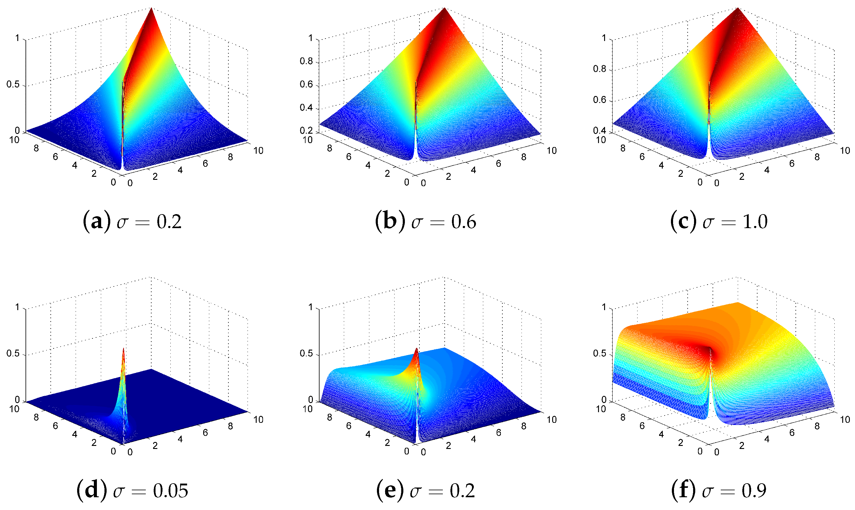
Second, spectral-similarity-based kernels, namely SAM-RBF and SID-RBF, are illustrated in Figure 2, which reveals that they combine the characteristics of both local and global kernels. The SAM-RBF kernel response on the whole increases as $x_1$ and $x_2$ increase overall. In this regard, it is similar to a global kernel. However, local kernels have distinct characteristics along the direction of $x_1$ or $x_2$. It should be noted that the properties of the local kernels are sensitive to the parameter of $\sigma$. When $\sigma$ increases from 0.2 to 1.0, as shown in Figure 2a–c, the shape of the SAM-RBF kernel exhibits a significant change in the gradient of the “watershed.”

As shown in Figure 2d–f, there is a distinct appearance in the form of a peak response for the SID-RBF kernel. Therefore, it also possesses the characteristics of a local kernel, which is weaker than the SAM-RBF kernel.

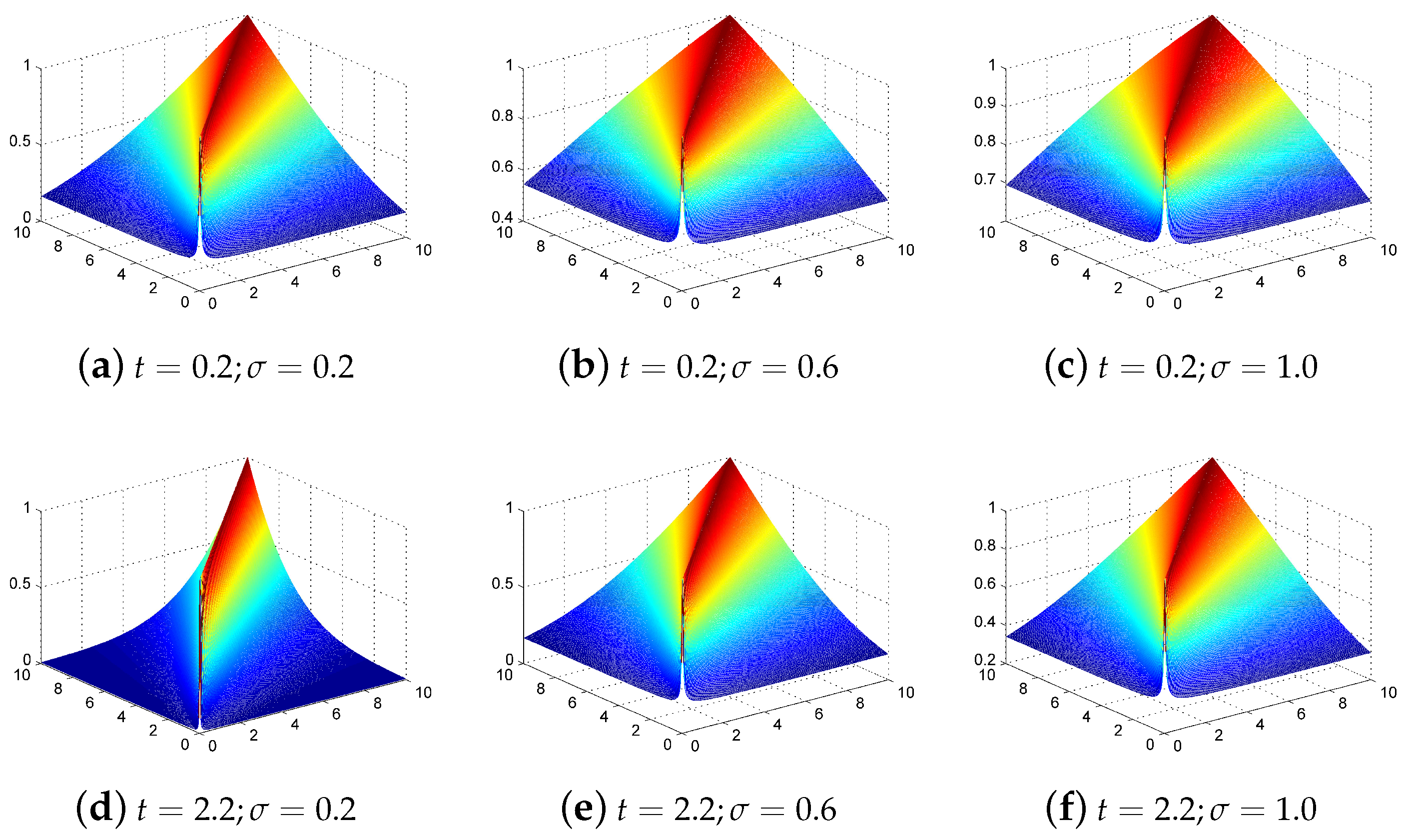
Third, the Power-SAM-RBF kernel requires two parameters, $\sigma (\sigma >0)$ and $t(t\in \mathrm{I}\mathrm{R})$, for controlling its performance. It is similar to the global kernel that the response of Power-SAM-RBF kernel increases with $x_1$ and $x_2$ increasing; meanwhile, it has the characteristic of local kernel, because the response along the vector of $[x_1,x_2]$ is higher than others. Therefore, there is a good blance between the capbility of interpolation and extrapolation. According to this, we can conclude the following:

• The characteristics of the global kernel become weaker and the characteristics of the local kernel become stronger when the power parameter of t increases. For example, when comparing Figure 3a,d, the saddle-backing along the watershed tends to shrink as t increases.
• With an increasing parameter of $\sigma$, the Power-SAM-RBF kernel exhibits more characteristics of a global kernel and fewer characteristics of a local kernel. As shown in Figure 3a–c, the response of the kernel becomes less pronounced as $\sigma$ increases.

As shown in Figure 4, one can see the Normalized-SID-RBF kernel also has the characteristics of the global kernel, because its response increases with $x_1$ and $x_2$ increasing. In the mean time, there is also the characteristics of the local kernel with the response along some direction being higher than others. The Normalized-SID-RBF kernel has more distinct characteristics of global kernels than the SID-RBF kernel. Debnath and Takahashi [60] claimed that the normalized kernel achieves better performance than the original kernel. However, regarding the characteristics of a local kernel, the direction of its ridge trends toward one of its dimensions such that data in other dimensions are ignored. This indicates that some features in the original data may not be fully operational during model training.

4. Experimental Results

4.1. Dataset Description

4.1.1. Indian Pines

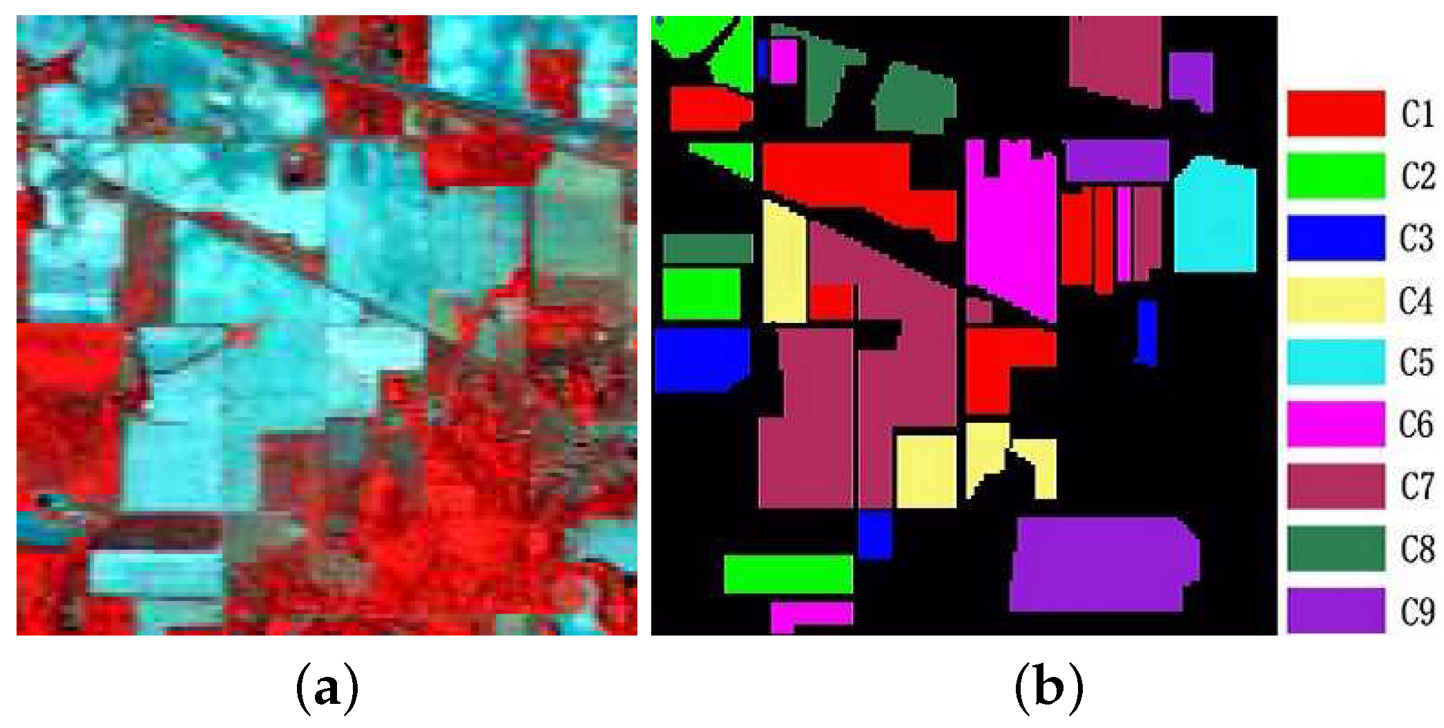
This dataset, which was acquired by an AVIRIS sensor, represents agricultural information from the Indian Pines test site in Northwestern Indiana, USA. After 20 water absorption bands are discarded, the image has a size of $145\times 145\times 220$. The spatial resolution is 20 m per pixel, and the spectral coverage ranges from 0.2 to 2.4 $\mathsf{\mu }$m. It contains 16 reference classes of crops (e.g., corn, soybean, and wheat). However, only nine classes were selected for our experiments because the number of samples in these nine classes (

Table 1. Ground truth classes for the Indian Pines dataset and their corresponding numbers of samples.

Label	Indian Pines	University of Pavia	Salinas Valley
C1	Corn-notill	Asphalt	Brocoli green weeds 1
C2	Corn-mintill	Meadows	Brocoli green weeds 2
C3	Grass-pasture	Gravel	Fallow
C4	Grass-trees	Trees	Fallow rough plow
C5	Hay-windrowed	Painted metal sheets	Fallow smooth
C6	Soybean-notill	Bare Soil	Stubble
C7	Soybean-mintill	Bitumen	Celery
C8	Soybean-clean	Self-Blocking Bricks	Grapes untrained
C9	Woods	Shadows	Soil vinyard develop
C10	-	-	Corn senesced green weeds
C11	-	-	Lettuce romaine 4wk
C12	-	-	Lettuce romaine 5wk
C13	-	-	Lettuce romaine 6wk
C14	-	-	Lettuce romaine 7wk
C15	-	-	Vinyard untrained
C16	-	-	Vinyard vertical trellis

) is greater than that in the other classes for model training. Figure 5a,b present color composites of the Indian Pines image and corresponding ground truth data, respectively.

4.1.2. University of Pavia

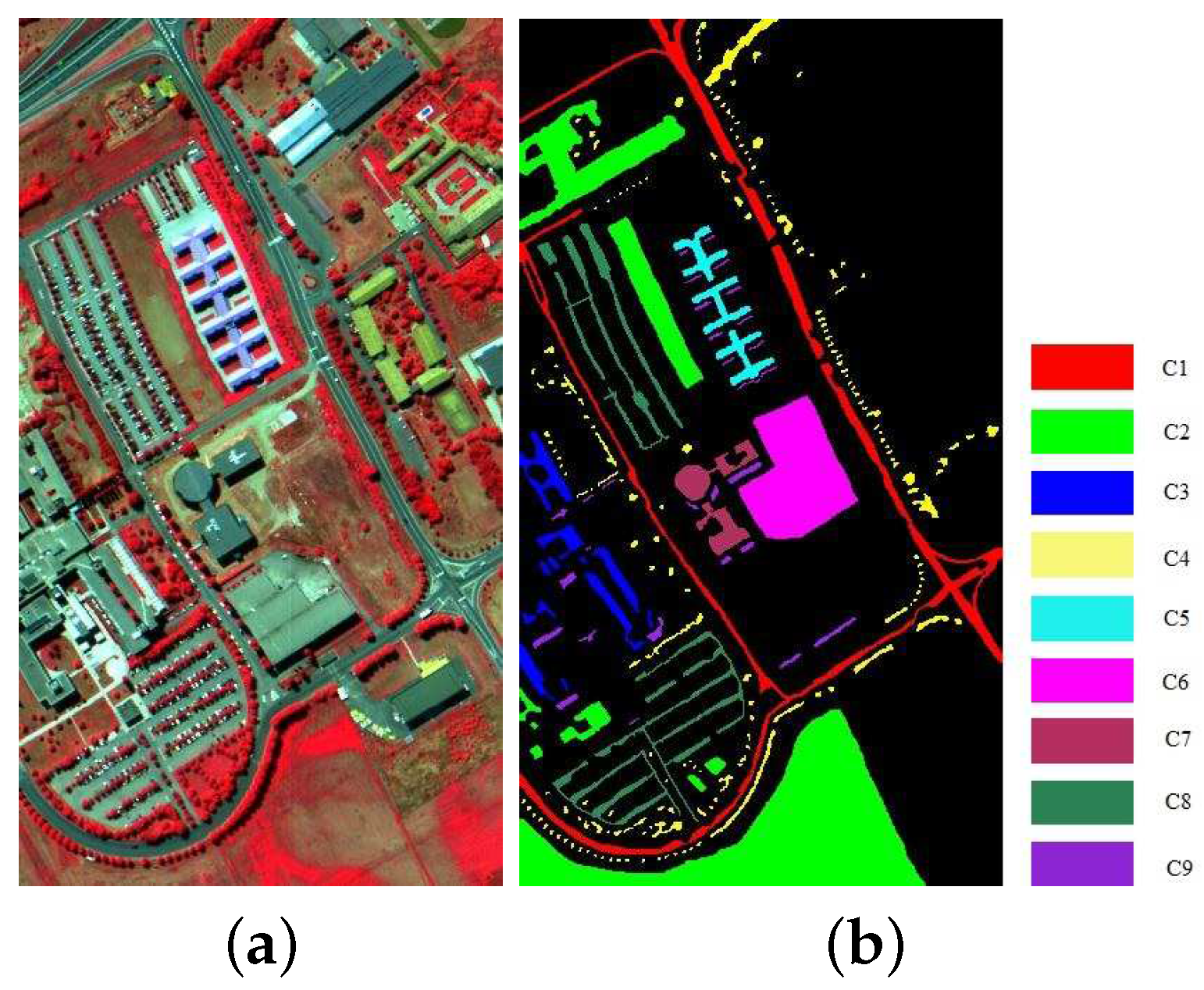
This dataset was acquired by the ROSIS instrument over the University of Pavia, Pavia, Italy in 2001. The image has a pixel resolution of $610\times 340$, spectral coverage ranging from 0.43 to 0.86 $\mathsf{\mu }$m, and spatial resolution of 1.3 m per pixel. After discarding noisy and water absorption bands, 103 spectral bands are retained. Figure 6a,b present a false color composite of the University of Pavia images and the corresponding ground-truth data, including nine classes of interest (Table 1).

4.1.3. Salinas Valley

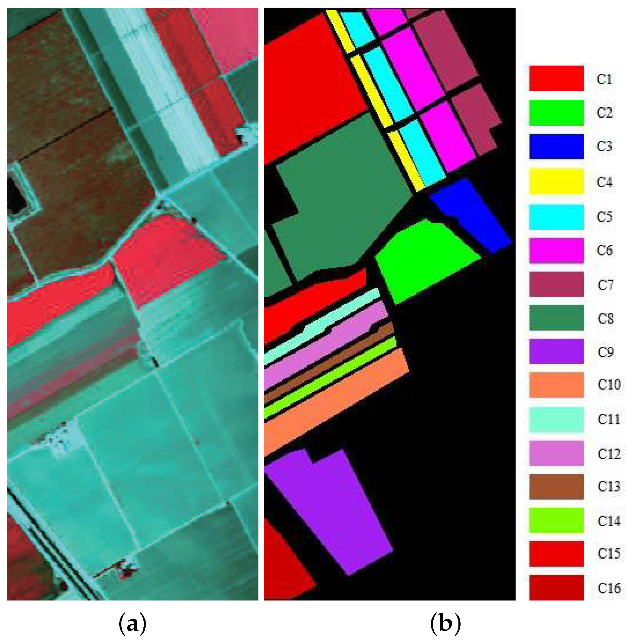
These images were collected by an AVIRIS sensor with a spatial resolution of 3.7 m per pixel over Salinas Valley, California, USA. The image size is $512\times 217$ pixels with 224 spectral bands. In our experiment, only 204 spectral bands were used after discarding noisy and water absorption bands. A total of 16 ground truth classes (Table 1) were considered. The false color compositions of bands 50, 30, and 20, and the ground truth map are presented in Figure 7a,b.

4.2. Experimental Setup

We evaluated the spectral-similarity-based kernels used for HSI classification using the following experimental settings:

• Training sample selection: $5\%$, $10\%$, $15\%$, and $20\%$ of samples randomly selected from the ground truth data as training samples.
• Classification accuracies: Five iteration classification experiments were conducted and the mean and variance of the overall accuracy (OA), average accuracy (AA), and Kappa coefficient were used for the evaluation. Additionally, the product accuracy (PA) for the experiments using the Indian Pines dataset was used for analysis. If $p_i$ is the number of correctly classified samples of the ith class, $t_i$ is the number of samples of the ith class in the ground-truth data, and N is the number of classes, then the OA, AA, and kappa coefficient can be defined as

  $$OA=\frac{\sum p_i}{\sum t_i},$$

  (36)

  $$AA=\frac{\sum \frac{p_i}{t_i}}{N},$$

  (37)

  $$Kappa=\frac{OA-\frac{\sum p_i\times t_i}{n}}{1-\frac{\sum p_i\times t_i}{n}}.$$

  (38)
• Methods: Six kernels for the SVM method, namely Linear-SVM, RBF-SVM, SAM-RBF, Power-SAM-RBF, SID-RBF, and Normalized-SID-RBF, were employed for classification experiments. The range of the parameters coef0 and $\gamma$ of the kernels was [0.01, 2000], and the range of the parameter of power t was [0.01, 5].
• Parameter optimization: Parameter optimization: We applied the PSO method to optimize the parameters of the SVM. The parameter settings for the PSO method, including the acceleration constants, maximum number of generations, and warm scale, are listed in

  Table 2. Parameter settings for the PSO method.

  Label	Class	Samples
  Acceleration constants	$c_1$ and $c_2$	1.5 and 1.7
  maximal number of generations	$MaxGen$	5
  Swarm scale	$SizePop$	10
  Inertia weight	$wV$	1
  Constriction factor	k	1

  .

4.3. Results for the Indian Pines Dataset

Table 3. Overall accuracies (OA), average accuracies (AA), kappa coefficients of Linear, RBF, SAM-RBF, Power-SAM-RBF, SID-RBF, and Normalized-SID-RBF kernels on the Indian Pines dataset.

Training Sample	Accuracies	Linear Kernel	RBF Kernel	SAM-RBF Kernel	Power-SAM-RBF Kernel	SID-RBF Kernel	Normalized-SID-RBF Kernel
5%	OA	75.33 ± 1.25	77.20 ± 1.33	77.50 ± 0.72	78.05 ± 0.76	72.90 ± 3.69	73.28 ± 1.99
	AA	75.55 ± 1.23	78.07 ± 1.26	76.03 ± 0.97	76.65 ± 0.96	72.17 ± 3.52	71.61 ± 3.01
	Kappa	0.7079 ± 0.0142	0.7309 ± 0.0152	0.7317 ± 0.0090	0.7389 ± 0.0092	0.6803 ± 0.0420	0.6830 ± 0.0245
10%	OA	80.58 ± 0.54	82.64 ± 0.45	83.09 ± 0.42	83.49 ± 0.76	77.10 ± 1.87	73.19 ± 4.47
	AA	80.95 ± 0.75	83.23 ± 0.81	82.58 ± 0.67	83.10 ± 1.11	77.23 ± 2.12	72.73 ± 4.30
	Kappa	0.7783 ± 0.0193	0.8020 ± 0.0188	0.8042 ± 0.0068	0.8091 ± 0.0053	0.7408 ± 0.0384	0.6912 ± 0.0619
15%	OA	82.16 ± 0.52	84.37 ± 0.60	85.42 ± 0.27	85.73 ± 0.36	77.15 ± 1.01	75.13 ± 1.94
	AA	82.88 ± 0.39	85.34 ± 0.64	85.66 ± 0.19	86.11 ± 0.43	76.91 ± 0.80	74.27 ± 1.90
	Kappa	0.7892 ± 0.0060	0.8154 ± 0.0073	0.8276 ± 0.0031	0.8314 ± 0.0043	0.7311 ± 0.0112	0.7068 ± 0.0226
20%	OA	83.72 ± 0.50	86.42 ± 0.40	87.44 ± 0.57	87.80 ± 0.48	79.13 ± 0.86	77.46 ± 2.45
	AA	84.68 ± 0.90	87.74 ± 0.57	87.83 ± 0.44	88.24 ± 0.33	79.04 ± 0.70	76.30 ± 3.02
	Kappa	0.8079 ± 0.0064	0.8400 ± 0.0050	0.8518 ± 0.0067	0.8561 ± 0.0056	0.7548 ± 0.0100	0.7341 ± 0.0289

presents a comparison of all kernels on the Indian Pines dataset in terms of OA, AA, and kappa coefficients with different ratios ($5\%$, $10\%$, $15\%$, and $20\%$) of training set.

The Power-SAM-RBF kernel generally performs better than the other kernels, particularly in terms of OA and kappa coefficient. When the percentage of training is high, it obtains the highest AAs among all kernels. The SAM-RBF kernel can be regarded as the second-best among all kernels considered. The only time the RBF kernel performs best is in terms of AA with a small proportion of training samples. Regardless, RBF is the third-best kernel overall. The SID-RBF and Normalized-SID-RBF kernels perform worse than the other four kernels for all proportions of training data.

Regarding the spectral-similarity-based kernels, the Power-SAM-RBF and SAM-RBF kernels yield impressive performance for all proportions of training set, but particularly for the high proportions of training data ($15\%$ or $20\%$). For all proportions of the training set, these two kernels outperform the other kernels in terms of OA and kappa coefficient. When the proportion of the training set is greater than $10\%$, the AAs of these two kernels rapidly exceed those of the RBF kernel. However, the performances of the SID-RBF and Normalized-SID-RBF kernels are less promising on the Indian Pines dataset for all proportions of training sample.

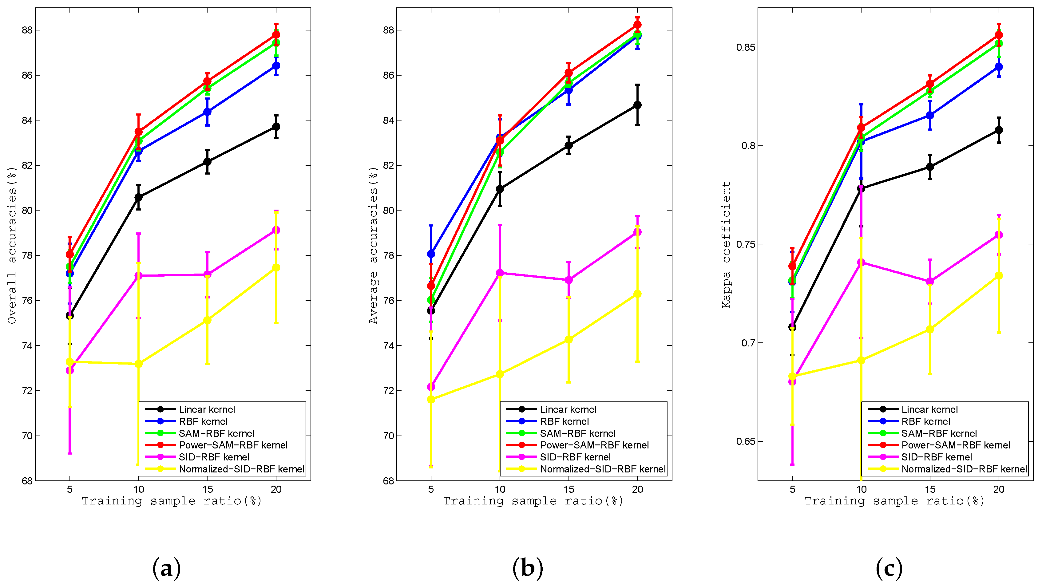
Figure 8 plots the curves of OA, AA, and kappa coefficient of the classification results of all kernels with proportions of training data ranging from $5\%$ to $20\%$. The superiority of the Power-SAM-RBF and SAM-RBF kernels becomes more obvious as the proportion of training data increases.

Considering the Power-SAM-RBF kernel as an example, regarding the kappa coefficient, when the proportion of training data is $5\%$, the value of the Power-SAM-RBF (0.7389) kernel is $0.8\%$ higher than that of the RBF kernel (0.7309). When the proportion of training data is $20\%$, the value of the Power-SAM-RBF kernel (0.8561) is $1.61\%$ higher than that of the RBF kernel (0.8400). The improvement in terms of OA is $0.85\%$ (Power-SAM-RBF kernel $78.05\%$, RBF kernel $77.20\%$) for a proportion of $5\%$, and (Power-SAM-RBF $87.80\%$, RBF kerenel $86.42\%$) $1.38\%$ when the proportion is $20\%$.

4.4. Results from the University of Pavia Dataset

Table 4. OAs, AAs, kappa coefficients of the Linear, RBF, SAM-RBF, Power-SAM-RBF, SID-RBF, and Normalized-SID-RBF kernels on the University of Pavia dataset.

Training Sample	Accuracies	Linear Kernel	RBF Kernel	SAM-RBF Kernel	Power-SAM-RBF Kernel	SID-RBF Kernel	Normalized-SID-RBF Kernel
5%	OA	89.95 ± 0.16	90.97 ± 1.97	90.77 ± 0.32	91.40 ± 0.23	88.88 ± 0.57	83.96 ± 1.68
	AA	85.31 ± 0.58	86.65 ± 5.23	87.09 ± 0.50	88.14 ± 0.45	86.74 ± 0.62	82.91 ± 1.18
	Kappa	0.8651 ± 0.0022	0.8791 ± 0.0275	0.8761 ± 0.0045	0.8849 ± 0.0033	0.8520 ± 0.0076	0.7864 ± 0.0215
10%	OA	90.88 ± 0.12	92.01 ± 1.39	92.43 ± 0.30	92.75 ± 0.17	91.12 ± 0.54	83.23 ± 0.64
	AA	87.12 ± 0.35	87.95 ± 3.60	89.56 ± 0.41	90.08 ± 0.28	89.16 ± 0.71	83.60 ± 1.22
	Kappa	0.8780 ± 0.0016	0.8929 ± 0.0194	0.8989 ± 0.0040	0.9032 ± 0.0024	0.8819 ± 0.0071	0.7773 ± 0.0089
15%	OA	90.95 ± 0.13	93.01 ± 1.25	93.13 ± 0.07	93.56 ± 0.07	91.84 ± 0.27	84.53 ± 0.90
	AA	87.11 ± 0.31	90.00 ± 2.58	90.32 ± 0.19	91.00 ± 0.14	89.98 ± 0.36	84.29 ± 0.76
	Kappa	0.8790 ± 0.0017	0.9065 ± 0.0171	0.9083 ± 0.0010	0.9142 ± 0.0010	0.8916 ± 0.0036	0.7946 ± 0.0119
20%	OA	91.28 ± 0.13	92.89 ± 0.89	93.46 ± 0.19	93.86 ± 0.08	92.31 ± 0.45	84.61 ± 0.63
	AA	87.40 ± 0.33	89.71 ± 1.76	90.84 ± 0.44	91.50 ±0.06	90.35 ± 0.45	84.99 ± 0.74
	Kappa	0.8832 ± 0.0018	0.9049 ± 0.0124	0.9128 ± 0.0025	0.9182 ± 0.0010	0.8977 ± 0.0059	0.7958 ± 0.0086

reveals that the Power-SAM-RBF kernel also yields the best performance among all kernels for the University of Pavia dataset, Pavia, Italy. It achieves the highest OAs, AAs, and kappa coefficients for all proportions of training data. The Normalized-SID-RBF kernel yields the worst performance.

Regarding the performance of the spectral-similarity-based kernels, both the Power-SAM-RBF and SAM-RBF kernel achieve promising performance. The SID-RBF kernel performs worse than the Linear and RBF kernels when the proportion of training data is small. As the proportion increases, the accuracy of the SID-RBF improves significantly. For example, when the proportion of training data is $20\%$, its OA ($92.31\%$), AA ($90.35\%$), and kappa coefficient ($0.8977$) are distinctly higher than those of the Linear kernel (OA: $91.28\%$; AA: $87.40\%$; and kappa coefficient: $0.8832$), and close to those of the RBF kernel, although its AA is significantly higher than that of the RBF kernel ($89.71\%$). While the Normalized-SID-RBF kernel still underperforms, its performance on the University of Pavia dataset is better than that on the Indian Pines dataset.

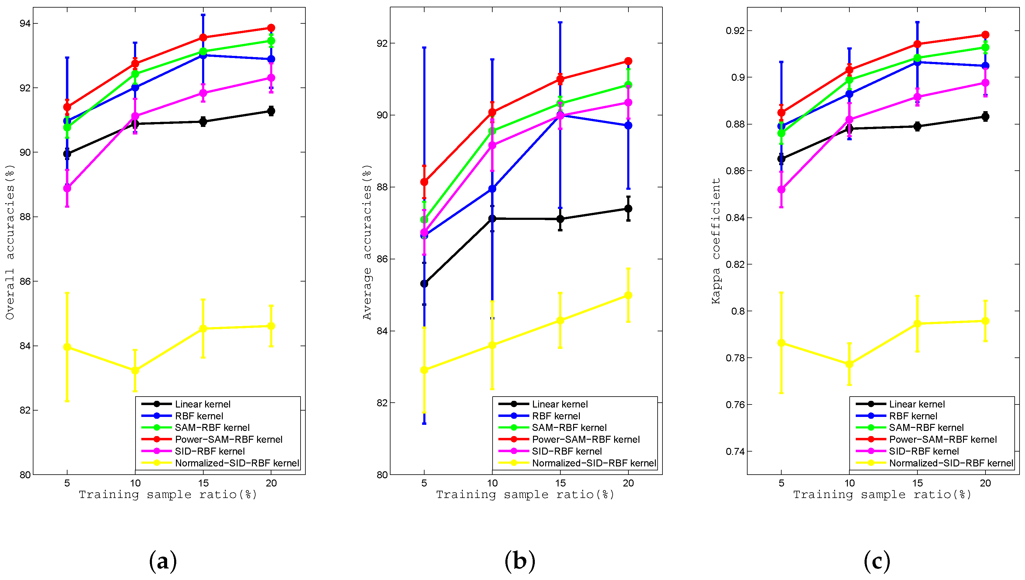
Figure 9 presents the curves of OA, AA, and kappa coefficient for all kernels and all proportions of training data on the University of Pavia dataset. The results reveal similar trends to those of the Indian Pines dataset. Overall, higher accuracies are achieved as the proportion of training data increases. Additionally, the Power-SAM-RBF and SAM-RBF kernels consistently provide the best performance.

The final comparison in Figure 9 is between the Linear and RBF kernels. Here, the superiority of the Power-SAM-RBF and SAM-RBF kernels also tends to increase with the proportion of training data. When the proportion of training data is $5\%$, the OA, AA, and kappa coefficient of the Power-SAM-RBF kernel are only $0.43\%$, $1.49\%$, and $0.58\%$, respectively. When the proportion of training data is $20\%$, the improvements of the Power-SAM-RBF kernel compared to the RBF kernel in terms of OA, AA, and the kappa coefficient are $0.97\%$, $1.79\%$, and $1.33\%$, respectively.

4.5. Results for the Salinas Valley Dataset

As shown in

Table 5. OAs, AAs, and kappa coefficients of the Linear, RBF, SAM-RBF, Power-SAM-RBF, SID-RBF, and Normalized-SID-RBF kernels on the Salinas Valley dataset.

Training Sample	Accuracies	Linear Kernel	RBF Kernel	SAM-RBF Kernel	Power-SAM-RBF Kernel	SID-RBF Kernel	Normalized-SID-RBF Kernel
5%	OA	92.10 ± 0.28	91.39 ± 0.27	91.15 ± 0.24	91.84 ± 0.15	88.96 ± 0.50	58.42 ± 4.83
	AA	95.65 ± 0.23	95.01 ± 0.26	94.73 ± 0.19	95.35 ± 0.31	93.36 ± 0.68	60.00 ± 3.68
	Kappa	0.9118 ± 0.0031	0.9039 ± 0.0030	0.9012 ± 0.0027	0.9090 ± 0.0017	0.8768 ± 0.0057	0.5410 ± 0.0506
10%	OA	92.73 ± 0.13	92.46 ± 0.68	92.55 ± 0.26	93.19 ± 0.28	90.13 ± 0.16	58.30 ± 5.58
	AA	96.47 ± 0.11	95.98 ± 0.46	95.88 ± 0.27	96.35 ± 0.25	94.25 ± 0.21	60.57 ± 3.96
	Kappa	0.9189 ± 0.0014	0.9159 ± 0.0077	0.9169 ± 0.0030	0.9241 ± 0.0031	0.8899 ± 0.0017	0.5398 ± 0.0600
15%	OA	93.05 ± 0.08	92.65 ± 0.55	93.32 ± 0.39	93.72 ± 0.14	89.62 ± 1.34	58.02 ± 6.51
	AA	96.70 ± 0.13	96.16 ± 0.29	96.41 ± 0.19	96.68 ± 0.10	94.74 ± 0.70	59.43 ± 4.32
	Kappa	0.9224 ± 0.0009	0.9180 ± 0.0062	0.9255 ± 0.0044	0.9300 ± 0.0015	0.8844 ± 0.0149	0.5366 ± 0.0692
20%	OA	93.09 ± 0.07	92.95 ± 0.37	93.53 ± 0.36	94.04 ± 0.12	89.67 ± 0.69	63.06 ± 8.99
	AA	96.83 ± 0.07	96.38 ± 0.13	96.60 ± 0.30	96.96 ± 0.15	95.18 ± 0.27	61.17 ± 5.31
	Kappa	0.9229 ± 0.0008	0.9213 ± 0.0042	0.9278 ± 0.0041	0.9336 ± 0.0014	0.8850 ± 0.0076	0.5896 ± 0.0969

, the Power-SAM-RBF kernel generally obtains the best performance on the Salinas HSI. For small proportions of training samples, the Power-SAM-RBF kernel performs better than the other kernels in terms of OA and kappa coefficient, but not in terms of AA, for which the Linear kernel exhibits the best performance. The SAM-RBF kernel achieves good classification results but not better than those of the Power-SAM-RBF kernel. The SID-RBF and Normalized-SID-RBF kernels exhibit the worst performance among all kernels for all proportions of training data.

Regarding the spectral-similarity-based kernels, the Power-SAM-RBF and SAM-RBF kernels achieve impressive performance, particularly for high proportions of training data. When the proportion of training data reaches $20\%$, the AA of the Power-SAM-RBF kernel ($96.96\%$) is greater those of the Linear ($96.83\%$) and RBF kernels ($96.38\%$). The OA and kappa coefficient of the Power-SAM-RBF kernel are $1.09\%$ and $1.23\%$ higher, respectively, than those of the commonly used RBF kernel. The OA and kappa coefficient of the SAM-RBF kernel are also higher than those of the Linear and RBF kernels. The performance of the SID-RBF and Normalized-SID-RBF kernels on the Salinas Valley dataset is still poor for all proportions of training data.

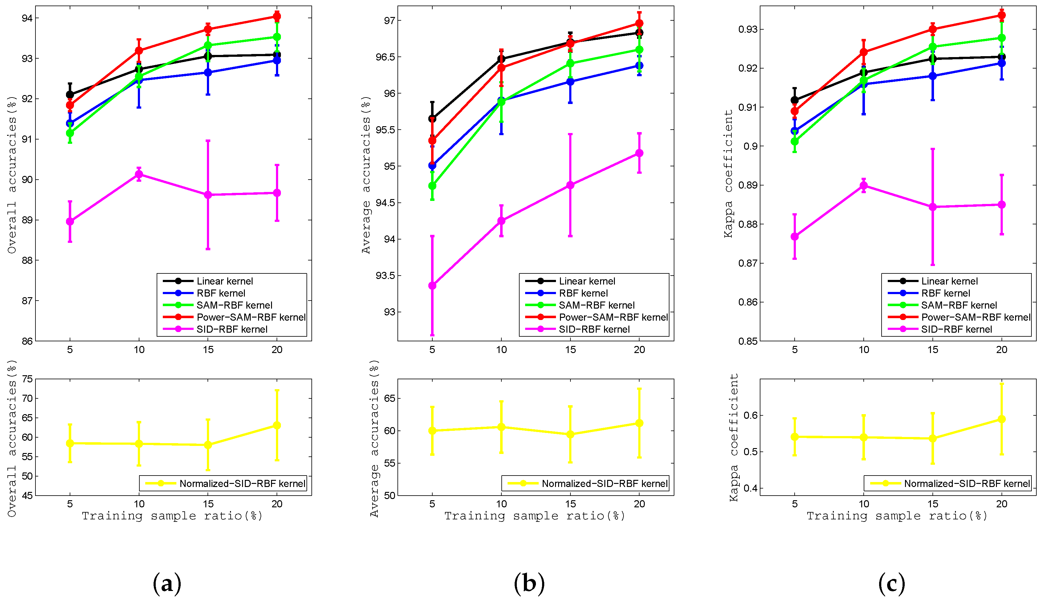
Similar to the experiment on the Indian Pines dataset, the Power-SAM-RBF kernel does not perform the best when the percentage of the proportion of training data is small. However, as shown in Figure 10, the superiority of the Power-SAM-RBF compared to the other kernels increases as the proportion of training data increases. When the proportion of training data is $5\%$, the OA, AA, and kappa coefficient of the Power-SAM-RBF kernel are lower than those of the RBF kernel. However, when the proportion of training data is $20\%$, the Power-SAM-RBF kernel outperforms the RBF-kernel in terms of OA, AA, and kappa coefficient by $1.09\%$, $0.58\%$, and $1.23\%$, respectively.

4.6. Effects of Similarity in Spectral Signatures

We noted that the improvement in terms of AA of the Power-SAM-RBF and SAM-RBF kernels compared to that of the Linear and RBF kernels is extremely different from that in terms of OA for different datasets. In the experiment on the Indian Pines and Salinas Valley datasets, the Power-SAM-RBF kernel exhibited stronger superiority over the RBF-kernel in terms of OA than in terms of AA. For example, when the proportion of training data is $20\%$, the OA of the Power-SAM-RBF kernel is $1.38\%$ higher than that of the RBF kernel, whereas the AA of the Power-SAM-RBF kernel is only $0.50\%$ higher than that of the RBF kernel. However, the superiority of the Power-SAM-RBF kernel over the RBF-kernel in terms of OA is less than that in terms of AA on the University of Pavia dataset. When the proportion of training data is $20\%$, the OA of the Power-SAM-RBF kernel is $0.97\%$ higher than that of the RBF kernel, while its AA is $1.71\%$ higher.

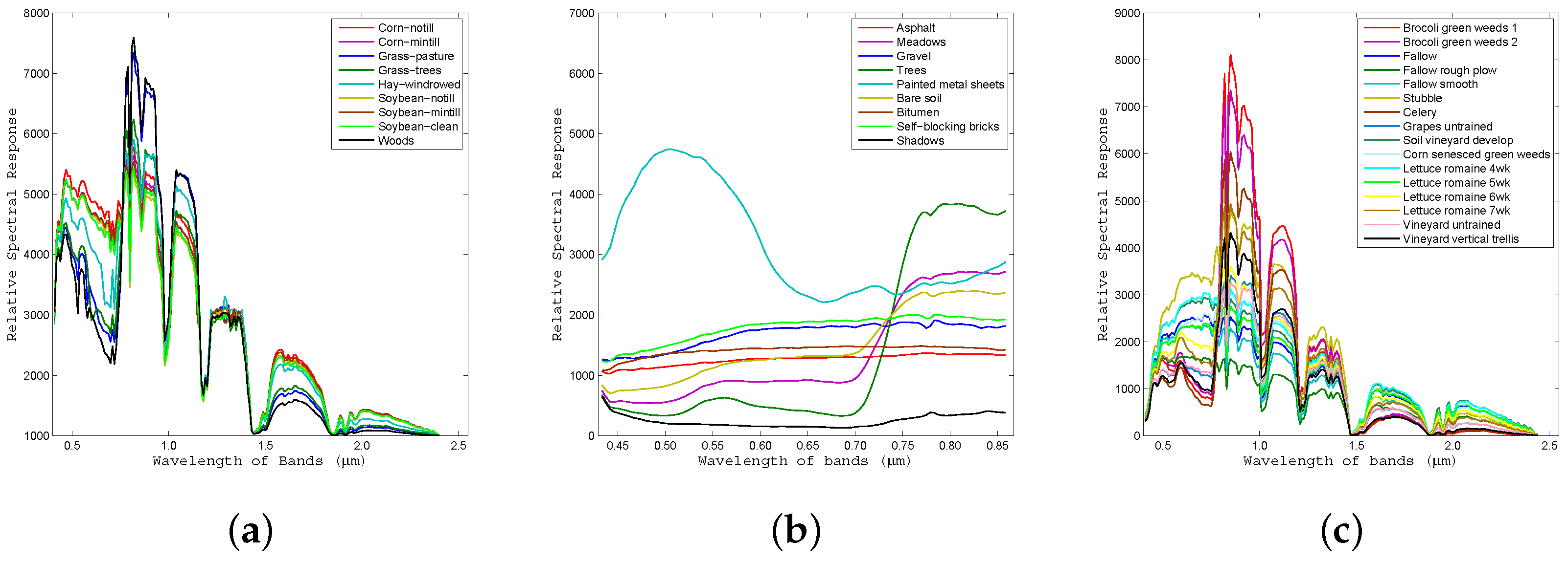
This indicates that the differences in kernel performance between the Indian Pines/Salinas Valley datasets and the University of Pavia dataset are relative to the original spectral signatures of these datasets. Figure 11 illustrates the average spectral signatures of each class from all labeled pixels in the ground-truth data. The differences between each spectral signature in the Indian Pines/Salinas Valley data can be clearly observed, as shown in Figure 11a,c, as well as for the University of Pavia data, as shown in Figure 11b. The higher spectral similarity of the Indian Pines/Salinas Valley datasets compared to that of the University of Pavia dataset indicates that the Power-SAM-RBF and SAM-RBF kernels are well suited to HSIs with low spectral similarity between each class. As a result, we can conclude that the superiority of the Power-SAM-RBF and SAM-RBF kernels compared with the RBF kernel is generally more pronounced when the discrimination between each spectral signature is increases.

To further validate the relationship between spectral similarity and classification accuracy, we consider the Indian Pines experimental results with proportions of training data of $5\%$ and $20\%$ as an example to compare the performances of the Power-SAM-RBF kernel and the commonly used RBF kernel. The sums of the five experimental results in the confusion matrices for the Indian Pines dataset with proportions of training data of $5\%$ and $20\%$ are listed in

Table 6. Summation of five experimental results in the confusion matrix for the Indian Pines dataset with a proportion of training data of $5\%$.

			Predicted Class
			C1	C2	C3	C4	C5	C6	C7	C8	C9
Ground truth class	RBF kernel	C1	4608	287	15	15	4	583	1219	54	0
		C2	253	2376	3	5	0	58	984	261	0
		C3	15	11	1980	88	27	21	12	35	106
		C4	6	0	71	3323	0	11	32	1	21
		C5	2	0	9	0	2259	0	0	0	0
		C6	401	65	21	4	2	3103	989	30	0
		C7	960	749	46	55	6	629	8949	265	1
		C8	255	224	9	11	0	236	597	1483	0
		C9	0	0	179	55	0	0	1	1	5774
	Power-SAM-RBF kernel	C1	4529	126	6	18	5	453	1522	126	0
		C2	329	2095	1	3	0	32	1155	325	0
		C3	8	5	1794	128	57	9	19	40	235
		C4	4	0	53	3348	12	1	16	9	22
		C5	2	0	7	4	2256	0	1	0	0
		C6	336	23	16	5	8	3171	1008	48	0
		C7	738	288	35	58	25	482	9907	127	0
		C8	468	233	4	5	0	98	767	1240	0
		C9	0	0	43	78	0	0	0	0	5889

and

Table 7. Summation of five experimental results in the confusion matrix for the Indian Pines dataset with a proportion of training data of $20\%$.

			Predicted Class
			C1	C2	C3	C4	C5	C6	C7	C8	C9
Ground truth class	RBF kernel	C1	4754	106	4	11	0	245	569	21	0
		C2	241	2392	0	2	0	12	583	90	0
		C3	7	3	1807	20	2	18	28	24	21
		C4	5	0	9	2874	0	2	22	0	8
		C5	2	0	4	0	1901	0	3	0	0
		C6	216	30	17	9	0	2903	714	1	0
		C7	632	272	32	31	2	427	8282	142	0
		C8	58	89	11	8	0	30	149	2025	0
		C9	0	0	46	32	0	0	6	0	4976
	Power-SAM-RBF kernel	C1	4682	72	3	13	0	278	591	71	0
		C2	178	2494	0	2	0	10	510	126	0
		C3	5	2	1775	44	5	10	28	23	38
		C4	1	0	29	2864	0	4	6	0	16
		C5	0	0	3	6	1900	1	0	0	0
		C6	250	13	11	11	0	3107	486	12	0
		C7	426	144	32	42	3	360	8710	103	0
		C8	137	85	7	5	0	29	201	1906	0
		C9	0	0	20	55	0	0	0	0	4985

, respectively.

We define the similarity between the spectral signatures of a pair of classes using the one-norm as follows:

$$S{S}_{pair}=\left|\right|S_{mean\_i}-S_{mean\_j}{\left|\right|}_1,$$

(39)

where $S_{mean\_i}$ and $S_{mean\_j}$ are the average spectral signatures of the ith and jth classes, respectively. The similarities between the spectral signatures of each pair of classes are listed in

Table 8. Similarity ($\times {10}^3$) between the spectral signatures of each pair of classes. Note that the high-similarity group is shown in green, the medium-similarity group is shown in yellow, and the low-similarity group is shown in red.

	C1	C2	C3	C4	C5	C6	C7	C8	C9
C1	-	1.7	11.4	7.9	5.0	2.6	1.7	2.5	13.2
C2	-	-	11.0	7.4	4.8	1.0	0.6	0.9	12.7
C3	-	-	-	4.1	6.8	11.5	11.4	11.1	2.1
C4	-	-	-	-	4.6	7.9	7.9	7.5	5.6
C5	-	-	-	-	-	5.4	5.2	4.9	8.6
C6	-	-	-	-	-	-	1.1	0.6	13.3
C7	-	-	-	-	-	-	-	1.1	13.3
C8	-	-	-	-	-	-	-	-	12.8
C9	-	-	-	-	-	-	-	-	-

. According to the similarity of such spectral signatures, we divided the signatures into three groups, namely high ($S{S}_{pair}<2\times {10}^3$), medium ($2\times {10}^3<S{S}_{pair}<10\times {10}^3$), and low ($S{S}_{pair}>10\times {10}^3$) similarity groups.

Given a confusion matrix T, the number of misclassified samples $T_{i,j}$b represents the number of samples in $C_i$ misclassified as class $C_j$. Based on the confusion matrix T of the Power-SAM-RBF and RBF kernel, we propose a definition of $Rati{o}_{PSR\_RBF}(i,j)$ to describe the improvement of the Power-SAM-RBF kernel compared to the RBF kernel as follows:

$$Rati{o}_{PSR\_RBF}(i,j)=\frac{PS{R}_{i,j}}{RB{F}_{i,j}}$$

(40)

where $PS{R}_{i,j}$ is the number of misclassified samples between classes i and j using the Power-SAM-RBF kernel, and $RB{F}_{i,j}$ is the number of misclassified samples between classes i and j using the RBF kernel. When $Rati{o}_{PSR\_RBF}(i,j)$ is lower than 1.0, this indicates that the Power-SAM-RBF kernel outperforms the RBF kernel. Otherwise, it indicates that the RBF kernel outperforms the Power-SAM-RBF kernel.

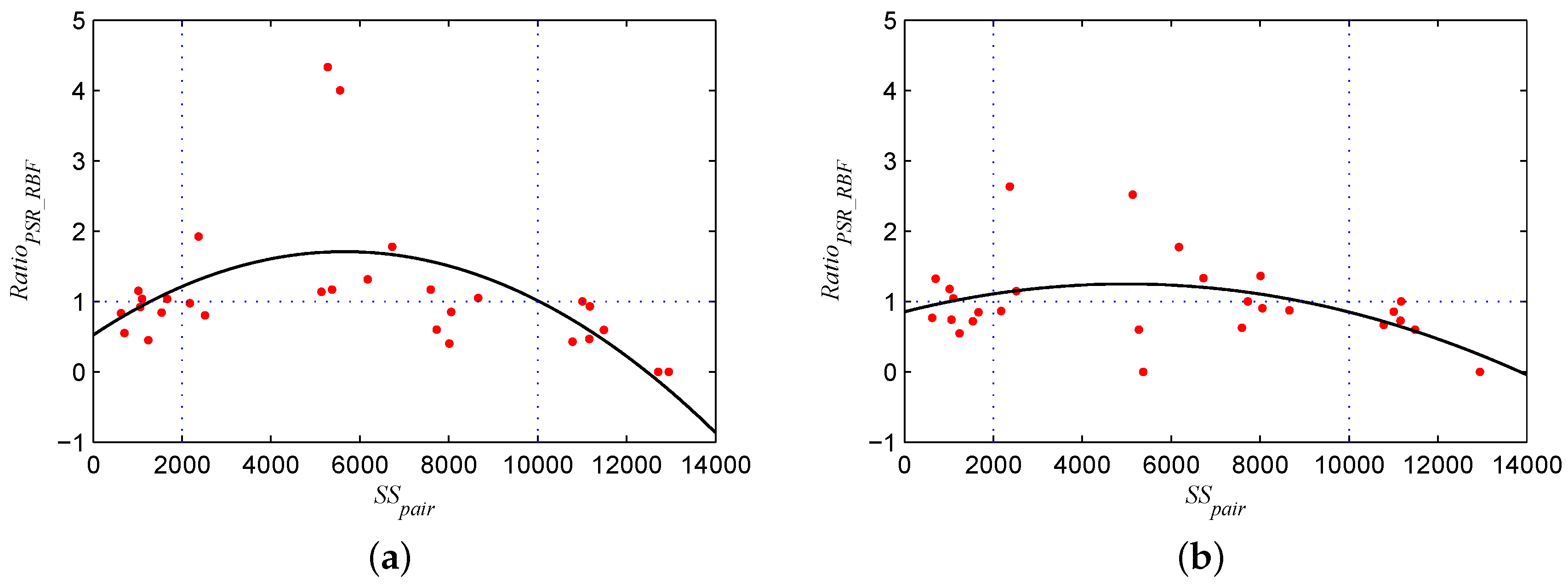
The calculated $Rati{o}_{PSR\_RBF}(i,j)$ results are plotted in Figure 12. Because the number of misclassified samples is zero for some pairs of classes, the results may be not a number (NaN) or infinity (Inf). (Figure 12 does not present these calculation results). There are seven and nine points missing in Figure 12a,b, respectively. Regardless, one can see that most of the class pairs (17 for the $5\%$ training set and 18 for the $20\%$ training set) have values less than or equal to 1.0. This indicates that the Power-SAM-RBF kernel is generally superior to the RBF kernel. Further details regarding this analysis are provided below.

As shown in Figure 12a,b, most of the $Rati{o}_{PSR\_RBF}(i,j)$ results are less than 1.0 when the $S{S}_{pair}$ is less than $2\times {10}^3$ or greater than $10\times {10}^3$. Specifically, all $Rati{o}_{PSR\_RBF}(i,j)$ resultsfor which the similarity of the corresponding class pair is greater than $10\times {10}^3$, are less than or equal to 1.0. This indicates that the Power-SAM-RBF kernel outperforms the RBF kernel when the similarity of class pairs is high or low. When the similarity of class pairs is moderate, the Power-SAM-RBF kernel is inferior to the RBF kernel. The quadratic fitting curves also validate this phenomenon.

Overall, the Power-SAM-RBF kernel is superior to the RBF kernel with either extremely high or low similarities between the spectral signatures of class pairs, whereas with moderate similarities of class pairs, it is inferior to the RBF kernel.

4.7. Effects of the Sizes of the Training Set

The experimental results for the three hyperspectral datasets discussed above support the theory that the superiority of the Power-SAM-RBF and SAM-RBF kernels compared to the Linear and RBF kernels becomes more evident as the size of the training set increases. In this section, we analyze the experimental results for the Indian Pines dataset again by comparing the Power-SAM-RBF and RBF kernels with different proportions of training samples. The numbers of samples for each class is listed in

Table 9. Ground truth classes for the Indian Pines dataset and their corresponding numbers of samples.

Class	Samples
C1	Corn-notill	1428
C2	Corn-mintill	830
C3	Grass-pasture	483
C4	Grass-trees	730
C5	Hay-windrowed	478
C6	Soybean-notill	972
C7	Soybean-mintill	2455
C8	Soybean-clean	593
C9	Woods	1265

.

Table 10. Average product accuracy (PA) for each class with the RBF and Power-SAM-RBF kernels with $5\%$ and $20\%$ proportions of training data.

Class	RBF Kernel		Power-SAM-RBF Kernel
	5%	20%	5%	20%
C1	67.91	83.26	66.75	82.00
C2	60.30	72.05	53.17	75.12
C3	86.27	93.63	78.17	92.00
C4	95.90	98.42	96.62	98.08
C5	99.52	99.53	99.38	99.48
C6	67.24	74.63	68.71	79.87
C7	76.75	84.34	84.97	88.70
C8	52.68	85.44	44.05	80.42
C9	96.07	98.34	97.99	98.52

lists the average PAs of each class for the RBF and Power-SAM-RBF kernels with proportions of training data of $5\%$ and $20\%$. When the proportion of training data is $5\%$, the PAs of the classes of C4, C6, C7, and C9 for the Power-SAM-RBF kernel are higher than those for the RBF kernel. When the PAs of the RBF kernel are compared to those of the Power-SAM-RBF kernel with a $20\%$ proportion of training data, the PAs of C2, C6, C7, and C9 for the Power-SAM-RBF kernel are higher than those for the RBF kernel. This indicates that the number of classes does not increase with an increase in the number of training samples. However, one can see that the PAs of C1, C3, C4, C5, and C8 for the Power-SAM-RBF kernel are close to those for the RBF kernel.

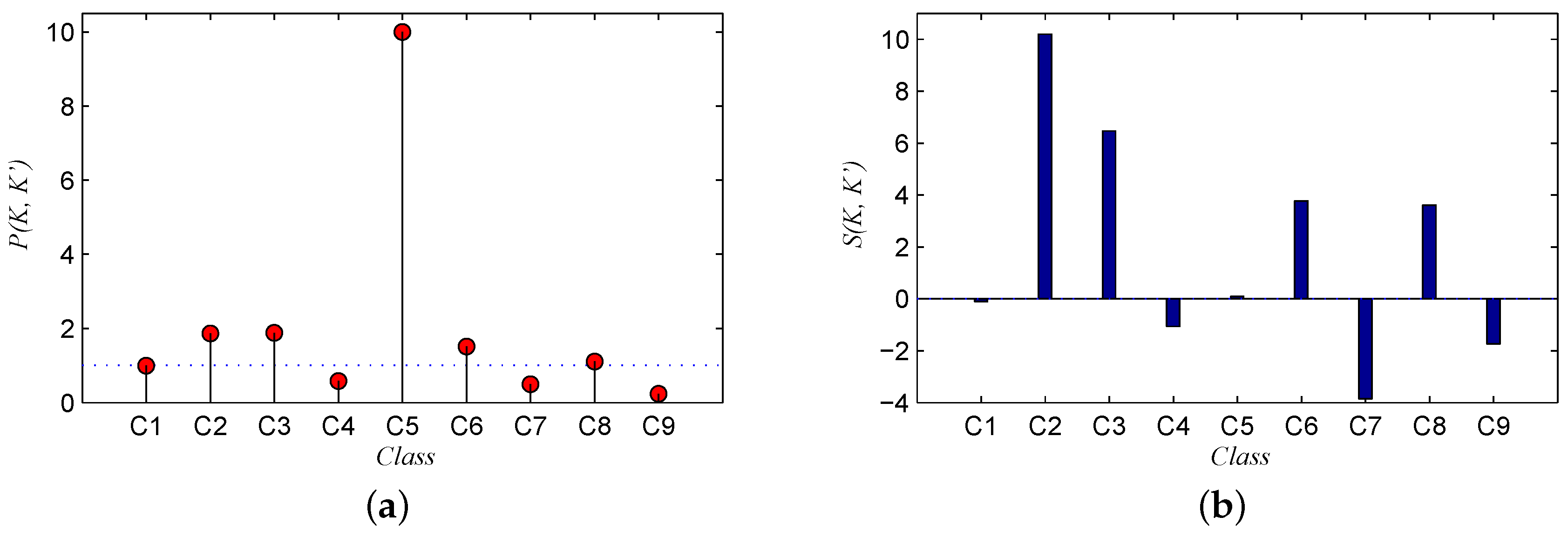
To demonstrate the superiority of the Power-SAM-RBF kernel to the RBF kernel with an increasing number of training samples, we define two indexes. Given that $AC{C}_{K,n}$ is the accuracy with a kernel of K with $n\%$ training samples for one class, the index $P_{K,K^{\prime }}$ represents the ratio of the accuracy improvement with a kernel k compared to that with another kernel $k^{\prime }$ when the number of training samples increases. Another index $S_{K,K^{\prime }}$ is used to represent the D-value of the superiority of a kernel k to another kernel $k^{\prime }$ when the number of training samples increases. Therefore, $P_{K,K^{\prime }}$ and $S_{K,K^{\prime }}$ can be defined as follows:

$$P_{K,K^{\prime }}=\frac{AC{C}_{K,n}-AC{C}_{K,n^{\prime }}}{AC{C}_{K^{\prime },n}-AC{C}_{K^{\prime },n^{\prime }}},$$

(41)

$$S_{K,K^{\prime }}=(AC{C}_{K,n}-AC{C}_{K^{\prime },n})-(AC{C}_{K,n^{\prime }}-AC{C}_{K^{\prime },n^{\prime }}).$$

(42)

If $P_{K,K^{\prime }}>1$, this indicates that the accuracy improvement with the kernel K is greater than that with the kernel $K^{\prime }$ when the number of training samples increases or decreases from $n^{\prime }$ to n. If $S_{K,K^{\prime }}>0$, this indicates that the accuracy improvement with the kernel k compared to that with the kernel $K^{\prime }$ with $n\%$ of training samples is greater than that with $n^{\prime }\%$ of training samples. In Figure 13, we have plotted the curves of $P_{K,K^{\prime }}$ and $S_{K,K^{\prime }}$ for the Power-SAM-RBF and RBF kernels when the proportion of training samples increases from $5\%$ to $20\%$, according to Table 8 and Equations (34) and (35).

Figure 13 indicates that when there are few original samples, the superiority of the Power-SAM-RBF kernel to the RBF kernel is more pronounced. The $P_{K,K^{\prime }}$ values of the Power-SAM-RBF kernel versus the RBF kernel for the classes of C2, C3, C5, C6, and C8 are all above 1.0. Additionally, the $S_{K,K^{\prime }}$ values of the Power-SAM-RBF kernel versus the RBF kernel for the class of C2, C3, C5, C6, and C8 are all above zero. Therefore, both $P_{K,K^{\prime }}$ and $S_{K,K^{\prime }}$ indicate the superiority of the Power-SAM-RBF kernel to the RBF kernel for the classes of C2, C3, C5, C6, and C8. As shown in Table 9, the sample numbers of C1, C7, and C9 are all above 1,000 and are the highest values among the nine classes. Therefore, the superiority of the Power-SAM-RBF kernel compared to the RBF kernel is proven to respond to increases in the number of training samples when the number of original samples is small.

5. Conclusions

In this study, we proposed two novel spectral-similarity-based kernels (Power-SAM-RBF and Normalized-SID-RBF kernels). Additionally, we demonstrated that four spectral-similarity-based kernels, namely the two proposed kernels, SAM-RBF kernel, and SID-RBF kernel, satisfy Mercer’s condition. Furthermore, a comparative analysis of these spectral-similarity-based kernels indicated that they have the characteristics of both local and global kernels. The SID-RBF and Normalized-SID-RBF kernels are non-isotropic. Therefore, the direction of the ridge trends toward one of the dimensions such that data with other dimensions are ignored. The Power-SAM-RBF and SAM-RBF kernels, which are isotropic, provide higher efficiency than the SID-RBF and Normalized-SID-RBF kernels.

HSIs of the Indian Pines, Pavia University, and Salinas Valley were used as experimental datasets. The results of using different proportions of the data for training revealed that the Power-SAM-RBF and SAM-RBF kernels achieve enhanced performance compared to the Linear, RBF, SID-RBF, and Normalized-SID-RBF kernels. The superiority of these two kernels, particularly the Power-SAM-RBF kernel, becomes more pronounced as the proportion of training data increases. For Indian Pines, when the percentage of training data is $20\%$, the OA, AA, kappa coefficient of Power-SAM-RBF kernel get the highest values of $87.80\%$, $88.24\%$, and 0.8561, respectively. For University of Pavia, when the percentage of training data is $20\%$, the OA, AA, kappa coefficient of Power-SAM-RBF kernel get the highest values of $93.86\%$, $91.50\%$, and 0.9182, respectively. For Salinas Valley, when the percentage of training data is $20\%$, the OA, AA, kappa coefficient of Power-SAM-RBF kernel get the highest values of $94.04\%$, $96.96\%$, and 0.9336, respectively.

Furthermore, we presented deep comparative analysis of the efficiency of the Power-SAM-RBF kernel in terms of the similarity of spectral signatures and size of the training set. First, according to the differences in the characteristics of the spectral signatures among the three hyperspectral datasets, we found that the superiority of the Power-SAM-RBF and SAM-RBF kernels over other kernels becomes more pronounced when a dataset has either extremely high or extremely low similarity among the spectral features of each class. Confusion matrices for the Power-SAM-RBF and RBF kernels in the Indian Pines experiment also confirmed this rule based on the analysis of three groups with different similarities of spectral signatures. Second, the PAs in the experimental results for the Indian Pines dataset with different numbers of training samples revealed that the increase in performance of the Power-SAM-RBF kernel versus the RBF kernel becomes more pronounced as the proportion of training samples increases.

In summary, there are three main conclusions to be drawn from this study. First, the spectral-similarity-based kernels discussed in this paper can satisfy Mercer’s condition. Additionally, the Power-SAM-RBF and SAM-RBF kernels for the SVM method can achieve significantly enhanced performance in terms of HSI classification, particularly the Power-SAM-RBF kernel. Second, either extremely high or extremely low similarities between the spectral signatures of different classes may yield better performance for the Power-SAM-RBF kernel compared to the other kernels. Finally, the Power-SAM-RBF kernel achieves even greater classification superiority with a larger training set compared to other kernels. The classification performance by using the proposed kernels for SVM is also not too distinct. Therefore, in a future study, we will employ spectral-similarity-based kernels in multiple-kernel methods to validate their efficiency in terms of HSI classification. Meanwhile, we will make efforts to explore more effective novel kernels for HSI classification.

References

1. Fauvel, M.; Tarabalka, Y.; Benediktsson, J.A.; Chanussot, J.; Tilton, J.C. Advances in spectral-spatial classification of hyperspectral images. Proc. IEEE 2013, 101, 652–675. [Google Scholar] [CrossRef] [Green Version]
2. Zhang, L.; Zhang, L.; Tao, D.; Huang, X. Sparse transfer manifold embedding for hyperspectral target detection. IEEE Trans. Geosci. Remote Sens. 2014, 52, 1030–1043. [Google Scholar] [CrossRef]
3. Du, B.; Zhang, L. Random-selection-based anomaly detector for hyperspectral imagery. IEEE Trans. Geosci. Remote Sens. 2011, 49, 1578–1589. [Google Scholar] [CrossRef]
4. Bioucas-Dias, J.M.; Plaza, A.; Dobigeon, N.; Parente, M.; Du, Q.; Gader, P.; Chanussot, J. Hyperspectral unmixing overview: Geometrical, statistical, and sparse regression-based approaches. IEEE J. Sel. Top. Appl. Earth Obs. Remote Sens. 2012, 5, 354–379. [Google Scholar] [CrossRef] [Green Version]
5. Landgrebe, D. Hyperspectral image data analysis. IEEE Signal Process. Mag. 2002, 19, 17–28. [Google Scholar] [CrossRef]
6. Shaw, G.; Manolakis, D. Signal processing for hyperspectral image exploitation. CVGIP Graph. Model Image Process. 2002, 19, 12–16. [Google Scholar] [CrossRef]
7. Hughes, G. On the mean accuracy of statistical pattern recognizers. IEEE Trans. Inf. Theory 1968, 14, 55–63. [Google Scholar] [CrossRef] [Green Version]
8. Jia, X.; Richards, J.A. Segmented prineipal components transformation for efficient hyperspectral remote sensing image display and classification. IEEE Trans. Geosci. Remote Sens. 1999, 37, 538–542. [Google Scholar]
9. Maghsoudi, Y.; Zoej, M.J.V.; Collins, M. Using class-based feature selection for the classification of hyperspectral data. Int. J. Remote Sens. 2011, 32, 4311–4326. [Google Scholar] [CrossRef]
10. Ham, J.; Chen, Y.; Crawford, M.M.; Ghosh, J. Investigation of the random forest framework for classification of hyperspectral data. IEEE Trans. Geosci. Remote Sens. 2005, 43, 492–501. [Google Scholar] [CrossRef] [Green Version]
11. Vapnik, V.N. The Nature of Statistical Learning Theory; Springer: NewYork, NY, USA, 1995. [Google Scholar]
12. Dundar, M.M.; Landgrebe, A. A cost-effective semisupervised classifier approach with kernels. IEEE Trans. Geosci. Remote Sens. 2004, 42, 264–270. [Google Scholar] [CrossRef]
13. Ben-Hur, A.; Horn, D.; Siegelmann, H.; Vapnik, V. Support vector clustering. Mach. Learn. Res. 2001, 2, 125–137. [Google Scholar] [CrossRef]
14. Rätsch, G.; Schökopf, B.; Smola, A.; Mika, S.; Onoda, T.; Müller, K.R. Robust ensemble learning. In Advances in Large Margin Classifiers; Smola, A., Bartlett, P., Schölkopf, B., Schuurmans, D., Eds.; MIT Press: Cambridge, MA, USA, 1999. [Google Scholar]
15. Camps-Valls, G.; Bruzzone, L. Kernel-based methods for hyperspectral image classification. IEEE Trans. Geosci. Remote Sens. 2005, 43, 1351–1362. [Google Scholar] [CrossRef]
16. Bharath, B.; Nicolasourty, C.; Sébastien, L. Sparse Hilbert Schmidt Independence Criterion and Surrogate-Kernel-Based Feature Selection for Hyperspectral Image Classification. IEEE Trans. Geosci. Remote Sens. 2017, 55, 2385–2398. [Google Scholar]
17. Fauvel, M.; Benediktsson, J.A.; Chanussot, J.; Sveinsson, J.R. Spectral and spatial classification of hyperspectral data using SVMs and morphological profiles. IEEE Trans. Geosci. Remote Sens. 2008, 46, 3804–3814. [Google Scholar] [CrossRef] [Green Version]
18. Li, J.; Marpu, P.R.; Plaza, A.; Bioucas-Dias, J.M.; Benediktsson, J.A. Generalized composite kernel framework for hyperspectral image classification. IEEE Trans. Geosci. Remote Sens. 2013, 51, 4816–4829. [Google Scholar] [CrossRef]
19. Gartner, T. A survey of kernels for structured data. CM SIGKDD Explor. 2003, 5, 49–58. [Google Scholar] [CrossRef]
20. Jaakkola, T.; Haussler, D. Exploiting generative models in discriminative classifiers. Adv. Neural Inf. Process. Syst. 1999, 10, 487–493. [Google Scholar]
21. Lodhi, H.; Saunders, C.; Shawe-Taylor, J.; Cristian-ini, N.; Watkins, C. Text classification using string kernels. J. Mach. Learn. Res. 2002, 2, 419–444. [Google Scholar]
22. Wahba, G.; Wang, Y.; Gu, C.; Klein, R.; Klein, B. Smoothing spline ANOVA for exponential families, with application to the Wisconsin Epidemiological Study of Diabetic Retinopathy. Ann. Stat. 1995, 23, 1865–1895. [Google Scholar]
23. Matérn, B. Spatial Variation; Springer: New York, NY, USA, 1960. [Google Scholar]
24. Swain, M.; Ballard, D. Color indexing. Int. J. Comput. Vis. 1991, 7, 11–32. [Google Scholar] [CrossRef]
25. Boughorbel, S.; Tarel, J.P.; Boujemaa, N. Conditionally positive definite kernels for SVM based image recognition. In Proceedings of the IEEE International Conference on Multimedia and Expo (ICME 2015), Amsterdam, The Netherlands, 6 July 2005; pp. 113–116. [Google Scholar]
26. Xie, L.; Li, G.; Xiao, M.; Peng, L.; Chen, Q. Hyperspectral Image Classification Using Discrete Space Model and Support Vector Machines. IEEE Geosci. Remote Sens. Lett. 2017, 14, 374–378. [Google Scholar] [CrossRef]
27. Xia, J.; Chanussot, J.; Du, P.; He, X. Rotation-Based Support Vector Machine Ensemble in Classification of Hyperspectral Data With Limited Training Samples. IEEE Trans. Geosci. Remote Sens. 2016, 54, 1519–1531. [Google Scholar] [CrossRef]
28. Collazos-Huertas, D.; Cardenas-Pena, D.; Castellanos-Dominguez, G. Instance-Based Representation Using Multiple Kernel Learning for Predicting Conversion to Alzheimer Disease. Int. J. Neural Syst. 2019, 29, 1850042-1–1850042-8. [Google Scholar] [CrossRef] [PubMed]
29. Dai, M.; Wang, S.; Zheng, D.; Na, R.; Zhang, S. Domain Transfer Multiple Kernel Boosting for Classification of EEG Motor Imagery Signals. IEEE Access 2019, 7, 49951–49960. [Google Scholar] [CrossRef]
30. Gautam, C.; Balaji, R.; Sudharsan, K.; Tiwari, A.; Ahuja, K. Localized Multiple Kernel learning for Anomaly Detection: One-class Classification. Knowl. Based Syst. 2019, 165, 241–252. [Google Scholar] [CrossRef] [Green Version]
31. Wilson, C.M.; Li, K.; Yu, X.; Kuan, P.; Wang, X. Multiple-kernel learning for genomic data mining and prediction. BMC Bioinform. 2019, 20, 241–252. [Google Scholar] [CrossRef] [Green Version]
32. Zhao, Y.; Song, Z.; Zheng, F. Learning a Multiple Kernel Similarity Metric for kinship verification. Inf. Sci. 2017, 430, 247–260. [Google Scholar] [CrossRef]
33. Wu, Y.; Yang, X.; Plaza, A.; Qiao, F.; Gao, L.; Zhang, B.; Cui, Y. Approximate Computing of Remotely Sensed Data: SVM Hyperspectral Image Classification as a Case Study. IEEE J. Sel. Top. Appl. Earth Obs. Remote Sens. 2016, 9, 5806–5818. [Google Scholar] [CrossRef]
34. Liu, L.; Huang, W.; Wang, C. Hyperspectral Image Classification With Kernel-Based Least-Squares Support Vector Machines in Sum Space. IEEE J. Sel. Top. Appl. Earth Obs. Remote Sens. 2018, 11, 1144–1157. [Google Scholar] [CrossRef]
35. Gu, Y.; Chanussot, J.; Jia, X.; Benediktsson, J.A. Multiple Kernel Learning for Hyperspectral Image Classification: A Review. IEEE Trans. Geosci. Remote Sens. 2017, 55, 6547–6565. [Google Scholar] [CrossRef]
36. Wang, Q.; Gu, Y.; Tuia, D. Discriminative multiple kernel learning for hyperspectral image classification. IEEE Trans. Geosci. Remote Sens. 2016, 54, 3912–3927. [Google Scholar] [CrossRef]
37. Gu, Y.; Liu, T.; Jia, X.; Benediktsson, J.A.; Chanussot, J. Nonlinear Multiple Kernel Learning with Multiple-Structure-Element Extended Morphological Profiles for Hyperspectral Image Classification. IEEE Trans. Geosci. Remote Sens. 2016, 54, 3235–3247. [Google Scholar] [CrossRef]
38. Gu, Y.; Gao, G.; Zuo, D.; You, D. Model selection and classification with multiple kernel learning for hyperspectral images via sparsity. IEEE J. Sel. Top. Appl. Earth Obs. Remote Sens. 2014, 7, 2119–2130. [Google Scholar] [CrossRef]
39. Liu, T.; Gu, Y.; Jia, X.; Benediktsson, J.A.; Chanussot, J. Classspecific sparse multiple kernel learning for spectral–spatial hyperspectral image classification. IEEE Trans. Geosci. Remote Sens. 2016, 54, 7351–7365. [Google Scholar] [CrossRef]
40. Freund, Y.; Schapire, R.E. A decision-theoretic generalization of on-line learning and an application to boosting. J. Comput. Syst. Sci. 1997, 55, 119–139. [Google Scholar] [CrossRef] [Green Version]
41. Kruse, F.A.; Lefkoff, A.B.; Boardman, J.W.; Heidebrecht, K.B.; Shapiro, A.T.; Barloon, P.J.; Goetz, A.F.H. The spectral image processing system (SIPS)–interactive visualization and analysis of imaging spectrometer data. Remote Sens. Environ. 1993, 44, 145–163. [Google Scholar] [CrossRef]
42. Chang, C.I. An information-theoretic approach to spectral variability, similarity, and discrimination for hyperspectral image analysis. IEEE Trans. Inf. Theory 2000, 46, 1927–1932. [Google Scholar] [CrossRef] [Green Version]
43. De Carvalho, J.; Meneses, O.A. Spectral correlation mapper (SCM): An improvement on the spectral angle mapper (SAM). In Proceedings of the Summaries of the 9th JPL Airborne Earth Science Workshop, Pasadena, CA, USA, 23–25 February 2000; JPL Publication: Pasadena, CA, USA, 2000; Volume 2, pp. 00–18. [Google Scholar]
44. Estrada, F.J.; Jepson, A.D. Spectral gradients: A material descriptor invariant to geometry and incident illumination. In Proceedings of the Seventh IEEE International Conference on Computer Vision, Kerkyra, Greece, 20–27 September 1999; Volume 2, pp. 861–867. [Google Scholar]
45. Richards, J.A.; Jia, X. Remote Sensing Digital Image Analysis, an Introduction; Springer: Berlin, Germany, 1999. [Google Scholar]
46. Du, Y.; Chang, C.I.; Ren, H.; D’Amico, F.M.; Jensen, J.O. New hyperspectral discrimination measure for spectral characterization. Opt. Eng. 2004, 43, 1777–1786. [Google Scholar]
47. Wang, K.; Gu, X.; Yu, T.; Lin, J.; Wu, G.; Li, X. Segmentation of high-resolution remotely sensed imagery combining spectral similarity with phase congruency. J. Infrared Millim. Waves 2013, 32, 73–79. [Google Scholar] [CrossRef]
48. Wang, K.; Yong, B.; Gu, X.; Xiao, P.; Zhang, X. Spectral similarity measure using frequency spectrum for hyperspectral image classification. IEEE Geosci. Remote Sens. Lett. 2015, 12, 130–134. [Google Scholar] [CrossRef]
49. He, Y.; Liu, D.; Yi, S. Recursive spectral similarity measure-based band selection for anomaly detection in hyperspectral imagery. J. Opt. 2010, 13, 015401. [Google Scholar] [CrossRef]
50. Yang, C.H.; Everitt, J.H. Using spectral distance, spectral angle and plant abundance derived from hyperspectral imagery to characterize crop yield variation. Precis. Agric 2012, 13, 62–75. [Google Scholar] [CrossRef]
51. Kumar, M.N.; Seshasai, M.V.R.; Prasad, K.S.V.; Kamala, V.; Ramana, K.V.; Dwivedi, R.S.; Roy, P.S. Nonparametric weighted feature extraction for classification. Int. J. Remote Sens. 2011, 32, 4041–4053. [Google Scholar]
52. Chauhan, H.J.; Mohan, B.K. Effectiveness of SID as Spectral Similarity Measure to Develop Crop Spectra from Hyperspectral Image. J. Indian Soc. Remote Sens. 2018, 46, 1853–1862. [Google Scholar] [CrossRef]
53. Zhang, W.; Li, W.; Zhang, C.; Li, X. Incorporating Spectral Similarity Into Markov Chain Geostatistical Cosimulation for Reducing Smoothing Effect in Land Cover Postclassification. IEEE J. Sel. Top. Appl. Earth Obs. Remote Sens. 2017, 10, 1082–1095. [Google Scholar] [CrossRef]
54. Mercier, G.; Lennon, M. Support vector machines for hyperspectral image classification with spectral-based kernels. In Proceedings of the IEEE Geoscience and Remote Sensing Symposium, Toulouse, France, 21–25 July 2003; Volume 1, pp. 288–290. [Google Scholar]
55. Fauvel, M.; Chanussot, J.; Benediktsson, J.A. Evaluation of kernels for multiclass classification of hyperspectral remote sensing data. In Proceedings of the IEEE International Conference on Acoustics, Toulouse, France, 14–19 May 2006; Volume 2, pp. 813–816. [Google Scholar]
56. Boughorbel, S. Kernels for Image Classification with Support Vector Machines. Ph.D. Thesis, Université de Paris-Sud, Orsay, France, 2005. [Google Scholar]
57. Mercer, J. Functions of Positive and Negative Type, And Their Connection with the Theory of Integral Equations. Philos. Trans. R. Soc. A Math. Phys. Eng. Sci. 1909, 209, 415–446. [Google Scholar]
58. Burges, C.J.C. A tutorial on support vector machines for pattern recognition. Data Min. Knowl. Discov. 1998, 2, 121–167. [Google Scholar] [CrossRef]
59. Smits, G.F.; Jordaan, E.M. Improved SVM regression using mixtures of kernels. In Proceedings of the International Joint Conference on Neural Networks, Honolulu, HI, USA, 12–17 May 2002; pp. 2785–2790. [Google Scholar]
60. Debnath, R.; Takahashi, G. Kernel selection for the support vector machine. IEICE Trans. Inf. Syst. 2004, E87-D, 2903–2904. [Google Scholar]
Figure 1. Polynomial and radial basis function (RBF) kernel representations. Polynomial kernels of degree (a) 2, (b) 3, and (c) 5; RBF kernels with the parameter σ of (d) 0.2, (e) 0.6, and (f) 1.0.
Remotesensing 12 02154 g001
Figure 2. Spectral angle mapper (SAM)-RBF kernel and spectral information divergence (SID)-RBF kernel representation. SAM-RBF kernel with parameter σ values of (a) 0.2, (b) 0.6, and (c) 1.0. SID-RBF kernel with parameter σ values of (d) 0.05, (e) 0.2, and (f) 0.9.
Remotesensing 12 02154 g002
Figure 3. Power-SAM-RBF kernel characteristics with different parameters of t and σ .
Remotesensing 12 02154 g003
Figure 4. Normalized-SID-RBF kernel representation with parameter σ values of (a) 0.05, (b) 0.2, and (c) 0.9.
Remotesensing 12 02154 g004
Figure 5. (a) False color hyperspectral remote sensing image over the Indian Pines test site (using bands 50, 27, and 17). (b) Ground truth of the labeled area with nine classes of land cover: Corn-notill, Corn-mintill, Grass-pasture, Grass-trees, Hay-windrowed, Soybean-notill, Soybean-mintill, Soybean-clean, and Woods.
Remotesensing 12 02154 g005
Figure 6. (a) False color hyperspectral data over the University of Pavia (using bands 105, 63, and 29). (b) Ground truth of the labeled area with nine classes of land cover: Asphalt, meadows, gravel, trees, painted metal sheets, bare soil, bitumen, self-blocking bricks, and shadows.
Remotesensing 12 02154 g006
Figure 7. (a) False color hyperspectral image (HSI) over Salinas Valley (using bands 68, 30, and 18); (b) Ground truth of the labeled area with 16 classes of land cover: Broccoli green weeds 1, Broccoli green weeds 2, Fallow, Fallow rough plow, Fallow smooth, Stubble, Celery, Grapes untrained, Soil vineyard develop, Corn senesced green weeds, Lettuce romaine 4 wk, Lettuce romaine 5 wk, Lettuce romaine 6 wk, Lettuce romaine 7 wk, Vineyard untrained, and Vineyard vertical trellis.
Remotesensing 12 02154 g007
Figure 8. Curves of the (a) OA, (b) AA, and (c) kappa coefficient for the Linear, RBF, SAM-RBF, Power-SAM-RBF, SID-RBF, and Normalized-SID-RBF kernels with proportions of training data of 5 % , 10 % , 15 % , and 20 % for the Indian Pines dataset.
Remotesensing 12 02154 g008
Figure 9. Curves of the (a) OA, (b) AA, and (c) kappa coefficient for the Linear, RBF, SAM-RBF, Power-SAM-RBF, SID-RBF, and Normalized-SID-RBF kernels for proportions of training data of 5 % , 10 % , 15 % , and 20 % for the University of Pavia dataset.
Remotesensing 12 02154 g009
Figure 10. Curves of (a) OA, (b) AA, and (c) kappa coefficient for the Linear, RBF, SAM-RBF, Power-SAM-RBF, SID-RBF, and Normalized-SID-RBF kernels with proportions of training data of 5 % , 10 % , 15 % , and 20 % for the Salinas Valley dataset.
Remotesensing 12 02154 g010
Figure 11. Average spectral signature of each class for all labeled pixels in the ground-truth data for the (a) Indian Pines, (b) University of Pavia, and (c) Salinas Valley datasets.
Remotesensing 12 02154 g011
Figure 12. Curves of R a t i o P S R _ R B F ( i , j ) when the training set being (a) 5 % and (b) 20 % .
Remotesensing 12 02154 g012
Figure 13. Curves of (a) P K , K (the ratio of the accuracy improvement with the kernel k to that with another kernel k ) and (b) S K , K (the D-value of the superiority of the kernel k over another kernel k ) for the Power-SAM-RBF kernel versus the RBF kernel for the Indian Pines dataset.
Remotesensing 12 02154 g013