A Visualization Tool for Flood Dynamics Monitoring Using a Graph-Based Approach

Abstract

Insights into flood dynamics, rather than solely flood extent, are critical for effective flood disaster management, in particular in the context of emergency relief and damage assessment. Although flood dynamics provide insight in the spatio-temporal behaviour of a flood event, to date operational visualization tools are scarce or even non-existent. In this letter, we distil a flood dynamics map from a radar satellite image time series (SITS). For this, we have upscaled and refined an existing design that was originally developed on a small area, describing flood dynamics using an object-based approach and a graph-based representation. Two case studies are used to demonstrate the operational value of this method by visualizing flood dynamics which are not visible on regular flood extent maps. Delineated water bodies are grouped into graphs according to their spatial overlap on consecutive timesteps. Differences in area and backscatter are used to quantify the amount of variation, resulting in a global variation map and a temporal profile for each water body, visually describing the evolution of the backscatter and number of polygons that make up the water body. The process of upscaling led us to applying a different water delineation approach, a different way of ensuring the minimal mapping unit and an increased code efficiency. The framework delivers a new way of visualizing floods, which is straightforward and efficient. Produced global variation maps can be applied in a context of data assimilation and disaster impact management.

1. Introduction

The emergence of several new Synthetic Aperture Radar (SAR) missions throughout the past decade has boosted the field of flood remote sensing. However, most studies focus on the development of new or improved flood mapping algorithms, which result in single date flood extents. These products fail to provide information on flood dynamics, which is crucial for several applications. For example, flood duration can be linked directly to the degree of economic losses and damages to structures [1,2,3,4] in the context of disaster impact assessment (emergency relief, damage assessment, insurance claims …). Moreover, data assimilation for hydrodynamic forecasting could be improved by preserving information-dense regions, while removing redundant points [5,6,7,8]. In this way it is possible to determine where, when, and how often remote sensing data should be acquired for flood extent assimilation to be most effective. [6]. With this research we aim at producing a unified flood map, not limited to just flood extent, but incorporating insights on dynamics.

In [9], a visualization/analysis framework was established for flood dynamics, combining objects and graphs. This approach was based on the research of [10,11]. In this letter, we have extended our previous work to cover larger areas. This allows for a new way of visualizing flood dynamics. In order to test the behavior of the workflow proposed in [9] at a larger scale, two floods were chosen which extent over larger areas. These two non-similar floods were chosen because of their different origin and evolution.

2. Data

2.1. Synthetic Aperture Radar Imagery

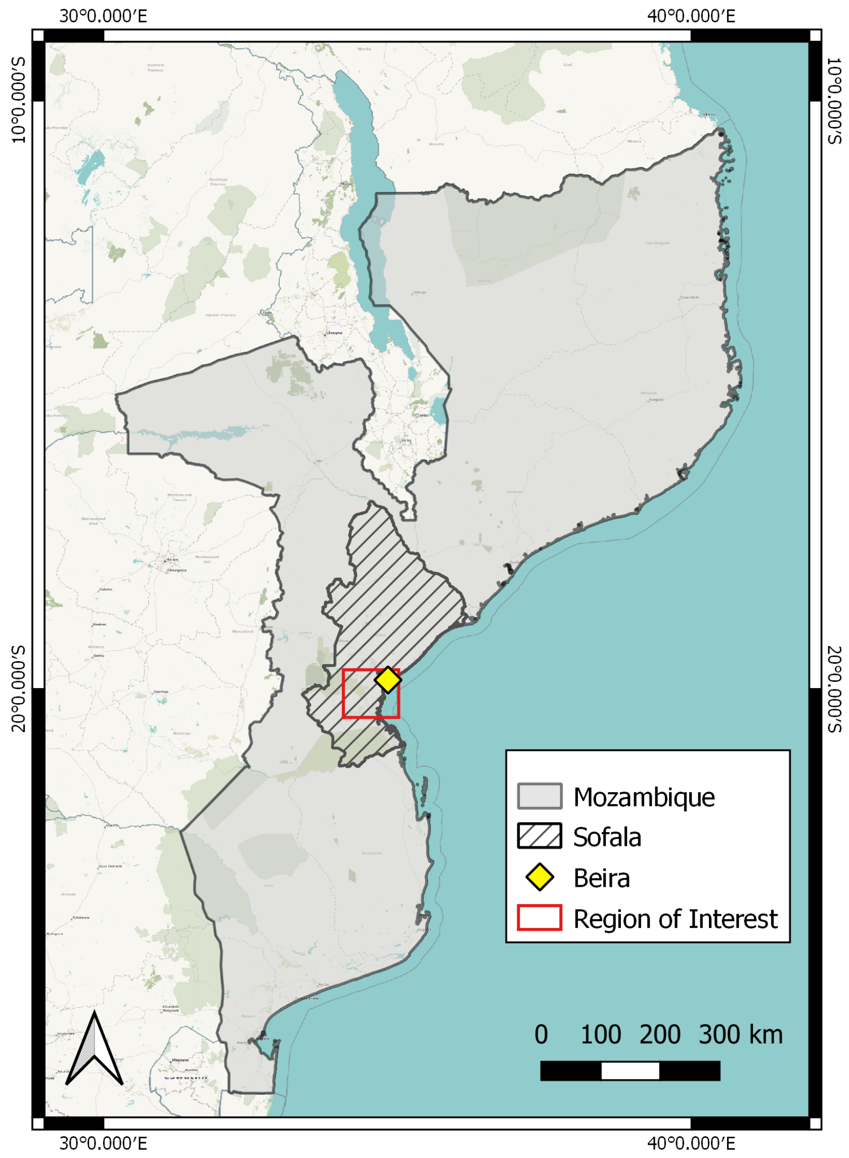
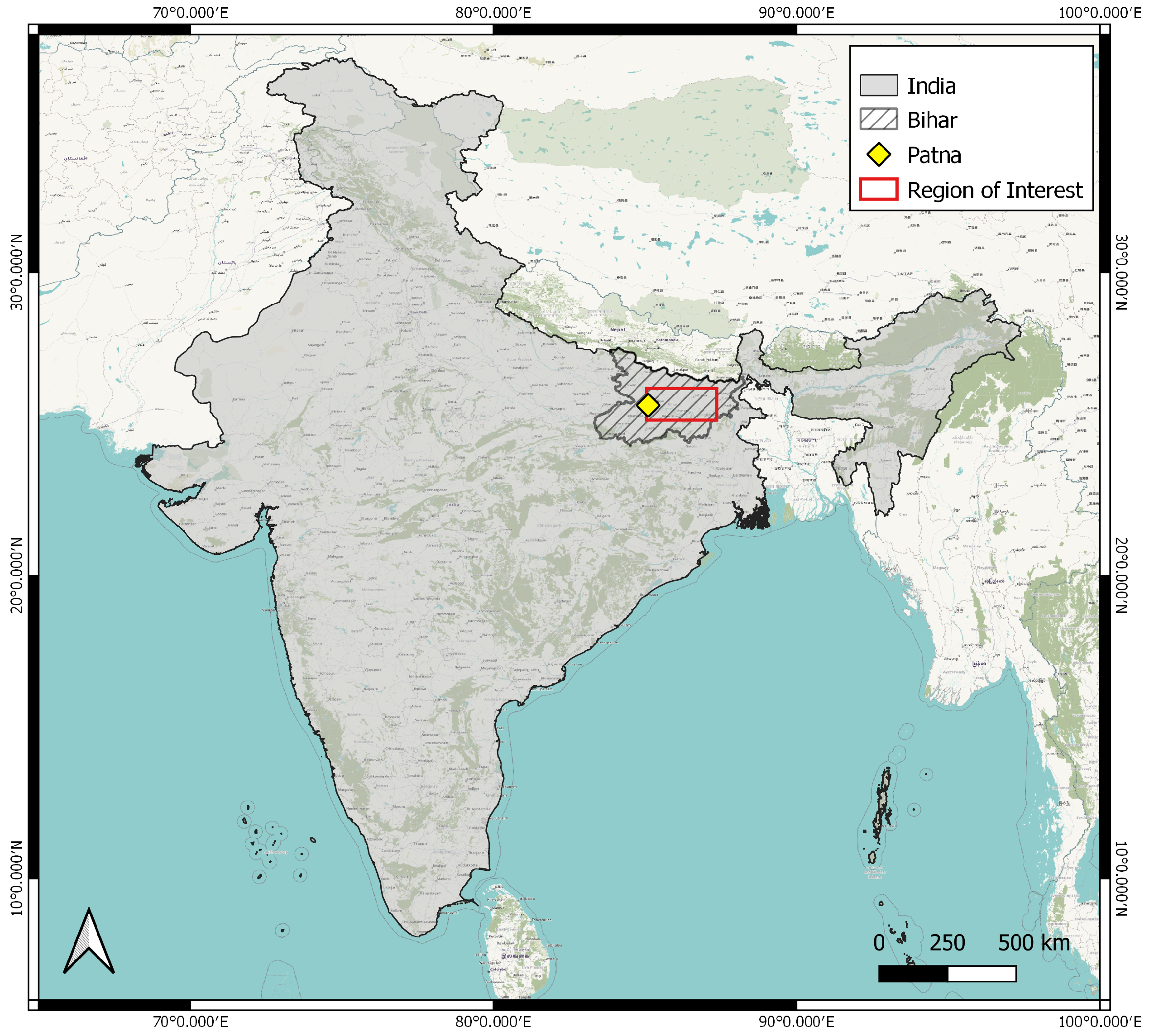
The Sentinel-1 mission from Copernicus, the European Union’s Earth observation program, provides C-band SAR imaging in a constellation of two polar-orbiting satellites. This constellation offers a 6 day exact repeat cycle at the equator. For this research, the Level-1 Ground Range Detected (GRD) products from the Interferometric Wide Swath (IW) acquisition mode are processed, which consist of focused SAR data that has been detected, multi-looked and projected to ground range using an Earth ellipsoid model. Only imagery captured during descending orbits is retained, because different orbits (ascending/descending) result in different radar shadows (among other distortions), generating artefacts upon comparison. For the IW mode, dual polarisation is available, i.e., Vertical transmit-Horizontal receive (VH) and Vertical transmit-Vertical receive (VV). The VV signal shows more consistent results due to the fact that the VV signal is more powerful, implying a higher signal-to-noise ratio, making thresholding easier (a small variation of the threshold will not result in big differences in flood extent) [12].

While selecting cases for upscaling, the following criteria were considered: (1) The flood area should be about 100 times larger than in the previous prove of concept [9]; (2) the images should fall completely within single Sentinel-1 captures in order to avoid stitching; (3) at least one external flood extent map should be available for comparison; (4) the cases should be different in nature to detect possible different behaviors. With these criteria, two recent floods were chosen, namely a flood in Mozambique and a flood in India, which both took place in the year 2019.

The first case is a flood caused by a tropical cyclone, Idai, which made landfall during the night of 14 to 15 March 2019 near Beira City, Sofala Province, in central Mozambique (Figure 1). This is a coastal area with mostly cropland and grassland areas, yet also some built up area (city of Beira). Sentinel-1 imagery (SAR IW GRD) is available (via Sentinel Hub [13]) on seven timesteps in the period between 2 March and 19 April 2019.

The second case is a flood which occurred between the 27 and 30 September 2019, caused by heavy rain in the East of India, in the State of Bihar, near the city of Patna (Figure 2). While India’s monsoon season normally starts to retreat by early September, heavy rainfall has continued here, triggering floods in many low-lying areas, resulting in waist-deep floodwaters [15]. For this case, Sentinel-1 imagery is available on eight timesteps in the period between 6 September and 30 October 2019.

2.2. Reference Data

While a ground truth is not available for these flood events, different “flood authorities” have produced flood extent maps for the regions of interest.

For the first case, Mozambique, we compare our results with flood maps from two external sources. The Luxembourg Institute of Science and Technology (LIST) provided us with a flood extent map for the Sofala region in Mozambique. They collaborate with the European Space Agency Research and Service Support Team (ESA RSS) for the production of automated Sentinel-1 based flood delineation products. The flood map is obtained by applying an automatic unsupervised change detection algorithm to pairs of Sentinel-1 images (pre-flood and during flood) [16]. The second source of flood maps for Mozambique is Disaster Charter [17], an initiative from ESA, The French National Centre for Space Studies (CNES) and The Canadian Space Agency (CSA), harvesting Earth observation assets from different space agencies. They provide flood maps at three timesteps for the Mozambique flood, based on Sentinel-1 imagery between 13 and 26 March 2019 over the Sofala province and its surroundings.

The second case, India, was compared with one external flood map, originating from Sentinel-Asia [18], a voluntary basis initiative led by the Asia-Pacific Regional Space Agency Forum (APRSAF) to support disaster management activity in the Asia-Pacific region. They provide a single-date flood map over the region of interest with a spatial resolution of 30 m × 30 m. The map is derived from SAR data acquired by Sentinel-1 satellites before (21 May 2019) and during (30 September 2019) the event.

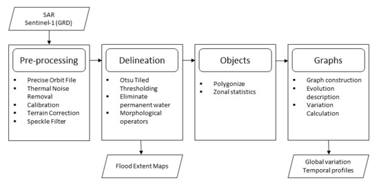
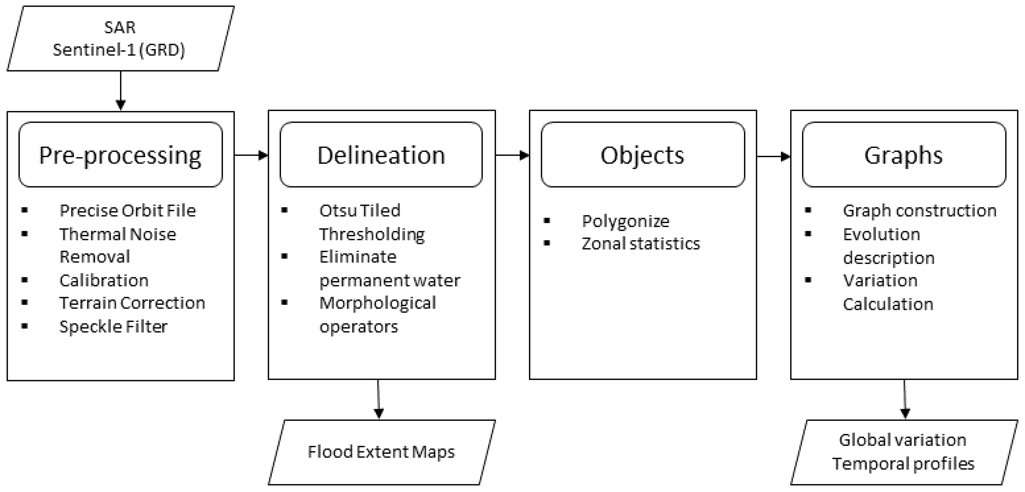
3. Method/Method Adaptations

Most of the workflow, presented in [9], has been retained for upscaling this research, yet some modifications were still necessary (Figure 3).

The Active contour modelling (ACM) sufficed for delineating water bodies in a small area [9], yet application of ACM on the current regions of interest leads to big over- and underestimations of the water extent. A more suitable way of obtaining the binary water maps was found by application of tiled thresholding using the Otsu algorithm [19]. This method selects a threshold by minimizing the within-class variance of two groups of pixels separated by the thresholding operator. It does not depend on modeling the probability density functions, and it assumes a bimodal distribution of gray-level values.

Permanent water bodies are then eliminated from the binary water maps by classifying pixels which are recognized as water in all timesteps, to permanent water, and excluding them from further evaluation.

In [9], the minimal mapping unit (MMU) was ensured by dropping all water polygons smaller than 16 pixels after polygonization. This however, results in a net loss of water area. For the current research, the MMU was obtained in a different way, i.e., by applying morphological operators [20]. First, a morphological closing reassigns non-water areas of maximum 4 by 4 pixels to water, if they are completely surrounded by water. Subsequently, morphological opening reassigns isolated water bodies smaller than 4 by 4 pixels non-water. In this way, the net loss of water area is compensated.

At this point, objects are created (‘Polygonize’ in Figure 3), reducing all detected water bodies to their individual extent and mean backscatter. Subsequently, they are grouped into entities (‘Graph construction’ in Figure 3) if they display spatial overlap on consecutive timesteps. Their evolution is then studied, based on the evolution of area and mean backscatter. This results in a different perception of the flood compared to a pixel-based analysis. Moreover, the analysis is simplified, which improves calculation time and ease of interpretation.

The evolution of each entity $o\ast$ is described by an evolution graph $G_o\ast$, which is a Directed Acyclic Graph (DAG), $G_0\ast =(V_0\ast ,E_0\ast )$. The nodes V represent the water bodies and the edges E represent their spatio-temporal overlap (from Khiali et al. [11]).

$$V_0\ast =\left\{o|o ϵ \vartheta , {\displaystyle \frac{\left|Pix\right(o\ast )\cap Pix(o\left)\right|}{\left|Pix\right(o\left)\right|}}\ge {\sigma }_1 or {\displaystyle \frac{\left|Pix\right(o\ast )\cap Pix(o\left)\right|}{\left|Pix\right(o\ast \left)\right|}}\ge {\sigma }_2\right\}$$

(1)

$$V_0\ast =\left\{o|o ϵ \vartheta , |Pix(o\ast )\cap Pix\left(o\right)|\ge 0\right\}.$$

(2)

$$E_0\ast =\left\{(o^i,o^j)|o^i ϵ O_t\cap V_o\ast ,o^j ϵ O_{t+1}\cap V_o\ast and Pix\left(o^i\right)\cap Pix\left(o^j\right)\ne ⌀\right\}.$$

(3)

Dynamics are quantified as follows [10]:

$$Var(G_i,G_{i+1})=\sum _{o_j\in G_i}{\displaystyle \frac{size\left(o_j\right)}{size\left(G_i\right)}}.{\displaystyle \frac{{\sum }_{o_k\in G_{i+1}}{w}_{j,k}.dist(o_j,o_k)}{{\sum }_k{w}_{j,k}}}.$$

(4)

Equation (4) describes the variation within one entity (graph) between timestep i and timestep $i+1$ as the weighted sum of variations of all polygons at timestep i, where these polygon variations are defined by the difference in backscatter with overlapping polygons from the next timestep ($i+1$), weighted by their amount of spatial overlap.

The global variation ($GlobVar$) for a graph represents the sum of the variations on each timestep (Equation (5)). The value of $GlobVar$ reflects the temporal behaviour of the entity, where high values indicate high spatio-temporal dynamics. Variation and global variation are unitless (Equations (4) and (5)).

$$GlobVar\left(G\right)=\sum _{i=1}^{n-1}Var(G_i,G_{i+1}).$$

(5)

4. Results

4.1. Pre-Processing and Thresholding

Results of pre-processing and Otsu tiled thresholding can be found in the Supplementary Materials. Since the external flood extent maps, presented in Section 2.2, are also associated with uncertainty, a statistical validation has been omitted. Only a visual comparison with external flood extent maps is executed. Based on this visual comparison, we conclude that the produced flood maps correspond well with the external flood maps and that these can be used for testing our algorithm. The results of these comparisons are only presented in the Supplementary Materials because the focus of this tool is on combining flood extent maps over a period of time and not on producing single date flood maps.

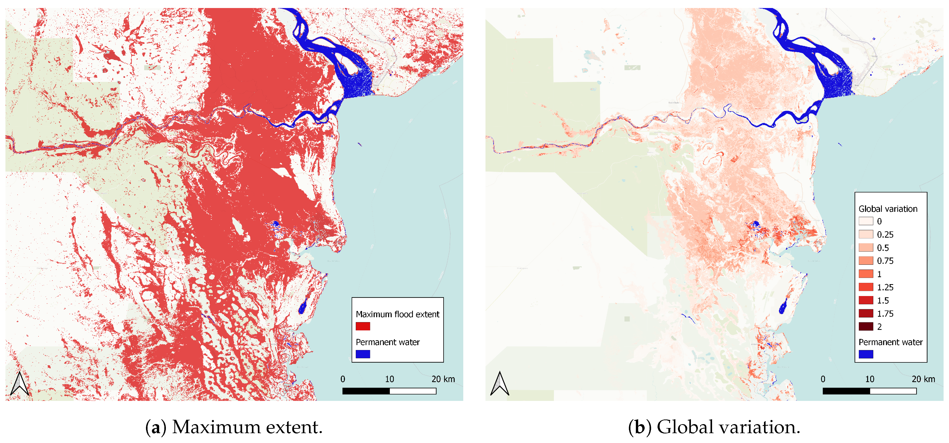
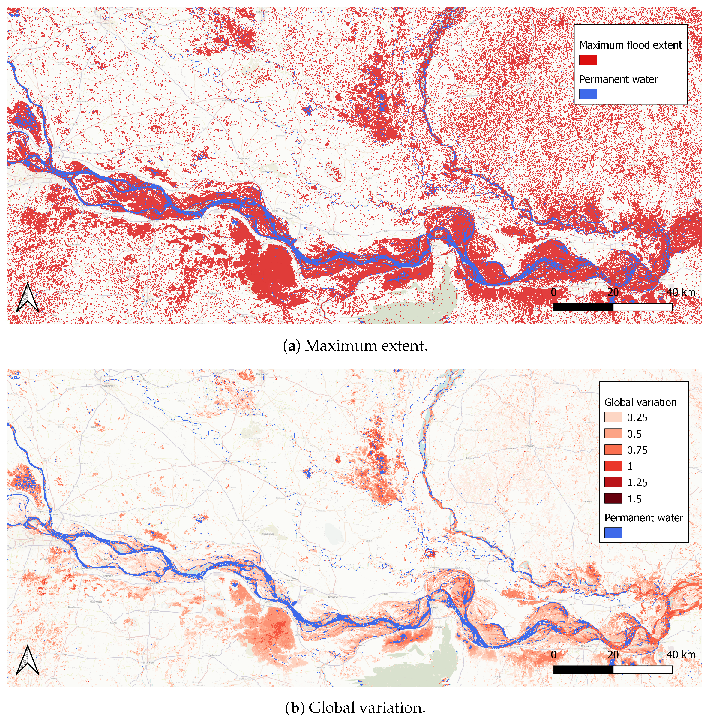
4.2. Global Variation Versus Maximum Flood Extent

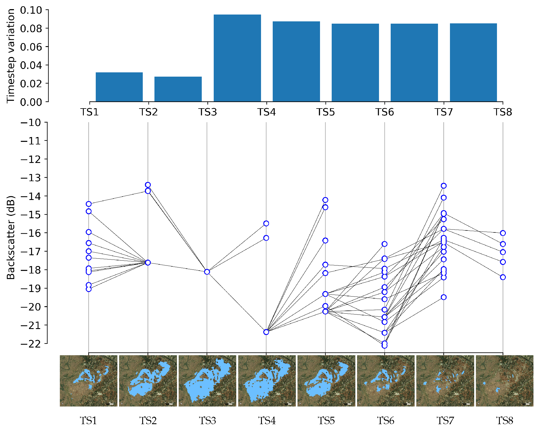
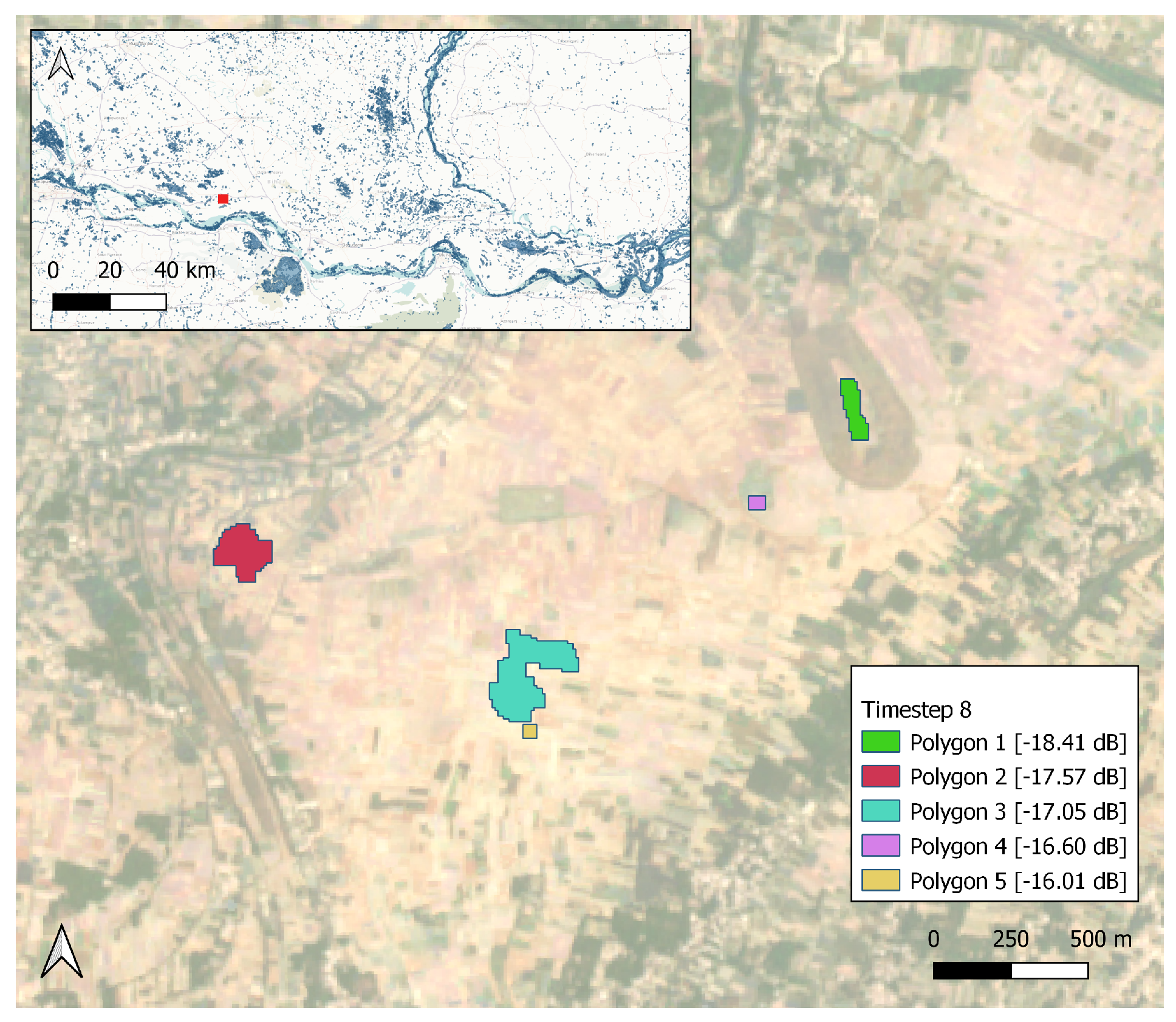
Variation is calculated for each timestep transition (available in Supplementary Materials) and summed to obtain global variation values. All maps presented throughout this article, are produced using EPSG:4326, the geodetic coordinate system for the world (with Datum “World Geodetic System 1984”, Ellipsoid “WGS 84” and prime meridian “Greenwich”).

When comparing the global variation map (Figure 4b) with the maximum flood extent (Figure 4a), the added value of this visualization becomes clear. The global variation map provides diversification within the flooded polygons. Because this method does not take into account ephemeral water bodies (i.e., areas which are flooded only on one timestep and do not overlap with other water areas on the previous or next timestep), the extent of variation (Figure 4b) is smaller than the maximum flood extent (Figure 4a).

The India flood is more dispersed (Figure 5) compared to the Mozambique flood (Figure 4b). The majority of the small water polygons is however ephemeral, and hence does not display a global variation value (Figure 5b). Most of the variation is displayed in the riverbed of the Ganges.

4.3. Graphs

Construction of graphs and variation calculation takes about 42 minutes for Case 1 (Mozambique, 7 timesteps) with an Intel(R) Core(TM) i7-4770 CPU @ 3.40GHz, 3401 Mhz, 4 Core(s), 8 Logical Processor(s). It took 6h24min for the second case. This is because of the dispersed nature of the India flood, forming a multitude of graphs (32505 graphs in Case 2 versus 2192 graphs in Case 1). Because of the object-based approach, an upscaling in area does not necessarily imply an increase of calculation time. However, the calculation time can be linked to the degree of dispersion. A dispersed flood will result in more entities, meaning more graphs and a higher calculation time. The Mozambique flood reaches a very large extent at the third timestep, combining previous separate entities in one big entity (one graph).

In Figure 6, the temporal profile of one entity is depicted (an additional example can be found in the Supplementary Materials). Each node in the graph represents a (flood) water polygon, while an edge depicts a spatial overlap between the connecting nodes. In this way, a water body is described by the evolution of the number of polygons and their backscatter over the timesteps. In Figure 7 the last timestep of Figure 6 is shown in detail. Five polygons are present at this timestep (TS8) with backscatter values ranging between −19 and −15 dB. These polygons form the nodes of the last timestep in the graph in Figure 6. Summing the timestep variations produces the global variation, depicted in Figure 5b. The timestep variation, depicted in the upper part of Figure 6, is assigned to the polygons prior to the transition. These timestep variations are available in the Supplementary Materials.

5. Discussion

This method was adapted to be operational on a larger scale: a different water delineation approach was applied (Otsu tiled thresholding), the minimal mapping unit was ensured in a different way (by application of morphological operators) and code efficiency was improved. This results in an innovative framework to visualize floods that is not only straightforward but also efficient. Depending on the flood type (disperseness), calculation times differ between 42 min and 6 h 24 min.

While the Mozambique flood occurs in a coastal zone and the India flood takes places inland, their global variation maps (Figure 4a and Figure 5b) show similarities. The majority of the high dynamic zones are located in or near the riverbeds (of the Buzi river in Mozambique and of the Ganges in India). This is not surprising because these areas are prone to flooding if the water level in the river rises. However the high dynamic zones are not restricted to the riverbeds only. These zones can point out interesting areas in the context of damage assessment and data assimilation.

Flood duration is a parameter often used for damage assessment in an agricultural [2,3] or urban context [4], for emergency relief or insurance claims. Because flood duration fails to incorporate spatio-temporal dynamics, we propose to combine both flood duration and (global) variation. If the flood duration parameter is not available, (global) variation values could be used as an operational parameter since they reflect the flood duration. In this way, variation values can be combined with land-use maps, road networks and population density maps in the context of emergency relief.

Calculated variation values could also be linked to the sensitivity of observation locations in a data assimilation framework, thereby improving flood predictions [5,6,7]. Observation targeting is a process in which supplementary observations are assimilated to improve the analysis in selected regions, and thereby reduce the uncertainty of a (flood) model [21]. When remotely sensed observations are used for data assimilation, thinning strategies are often applied to eliminate redundant information before the data assimilation [8]. Several authors determine their observation locations (whether or not for data assimilation purposes) on the basis of variances, be it model variance or observation variance [5,21,22]. In this way, observed (global) variation, calculated by the current framework, could function as an estimation for model variation in data scarce regions.

Finally, global variation results can be combined with the maximum flood extent in order to increase the understanding of the flood dynamics. It might even be interesting to add both maps, combining maximum flood extent (binary) and the global variation map in one unified flood extent/variation map. In this way, the area component can be combined with a dynamics component. The result of this approach is displayed in Figure 8 for the India flood.

6. Conclusions

In this letter we have successfully distilled a flood dynamics map from a radar SITS. The resulting global variation map evaluates floods, not only in terms of extent and duration, but also in terms of spatio-temporal variation. These insights into flood dynamics can therefore serve in operational frameworks for multiple applications. For example, this method can point out locations to be monitored to improve a hydraulic model (in the context of data assimilation) or the locations in need of damage relief (in the context of disaster management). Moreover, the framework is fast, effective and simple.

By using 2 exemplary flood cases, further upscaling is expected to go smoothly. Computation time increases with the number of entities, rather then with an increase in area. Since the method is generically deployable, it could be applied to different types of (natural) phenomena (e.g., snow, vegetation). Future research will include further upscaling to country/continent scale, analysis of longer timeseries, and inclusion of different sensors and platforms (e.g., Sentinel-2).

References

1. Rättich, M.; Martinis, S.; Wieland, M. Automatic flood duration estimation based on multi-sensor satellite data. Remote Sens. 2020, 12, 643. [Google Scholar] [CrossRef] [Green Version]
2. Ismail, M.S.; Md, A.N.; Ghazaly, M.D. A Study on the Effect of Flooding Depths and Duration on Soil Subgrade Performance and Stability. Int. J. 2020, 19, 182–187. [Google Scholar] [CrossRef]
3. O’Hara, R.; Green, S.; McCarthy, T. The agricultural impact of the 2015-2016 floods in Ireland as mapped through Sentinel 1 satellite imagery. Ir. J. Agric. Food Res. 2019, 58, 44–65. [Google Scholar] [CrossRef] [Green Version]
4. Wagenaar, D. The Significance of Flood Duration for Flood Damage Assessment. Master’s Thesis, Delft University of Technology, Delft, The Netherlands, 2012; pp. 1–104. [Google Scholar]
5. Van Wesemael, A.; Landuyt, L.; Lievens, H.; Verhoest, N.E. Improving flood inundation forecasts through the assimilation of in situ floodplain water level measurements based on alternative observation network configurations. Adv. Water Resour. 2019, 130, 229–243. [Google Scholar] [CrossRef]
6. Dasgupta, A.; Hostache, R.; Ramsankaran, R. Evaluating the Impact of Flood Extent Assimilation on Hydraulic Model Forecast Skill Results I: Flood Extent Evaluation Results II: Gauge Evaluation. In Proceedings of the 23rd International Congress on Modelling and Simulation (MODSIM2019), Canberra, Australia, 1–6 December 2019; pp. 3–4. [Google Scholar] [CrossRef]
7. Shastry, A.; Durand, M. Utilizing flood inundation observations to obtain floodplain topography in data-scarce regions. Front. Earth Sci. 2019, 6, 1–10. [Google Scholar] [CrossRef] [Green Version]
8. Ramachandran, R.; Li, X.; Movva, S.; Graves, S.; Greco, S.; Emmitt, D.; Terry, J.; Atlas, R. Intelligent thinning algorithm for earth system numerical model research and application. In Proceedings of the 85th AMS Annual Meeting, American Meteorological Society—Combined Preprints, San Diego, CA, USA, 9–13 January 2005; pp. 581–586. [Google Scholar]
9. Debusscher, B.; Van Coillie, F. Object-based flood analysis using a graph-based representation. Remote Sens. 2019, 11, 1883. [Google Scholar] [CrossRef] [Green Version]
10. Guttler, F.; Ienco, D.; Nin, J.; Teisseire, M.; Poncelet, P. A graph-based approach to detect spatiotemporal dynamics in satellite image time series. ISPRS J. Photogramm. Remote Sens. 2017, 130, 92–107. [Google Scholar] [CrossRef] [Green Version]
11. Khiali, L.; Ienco, D.; Teisseire, M. Object-oriented satellite image time series analysis using a graph-based representation. Ecol. Inform. 2018, 43, 52–64. [Google Scholar] [CrossRef] [Green Version]
12. DeVries, B.; Huang, C.; Armston, J.; Huang, W.; Jones, J.W.; Lang, M.W. Rapid and robust monitoring of flood events using Sentinel-1 and Landsat data on the Google Earth Engine. Remote Sens. Environ. 2020, 240, 111664. [Google Scholar] [CrossRef]
13. Sinergise Ltd. Copernicus Open Acces Hub. Available online: https://scihub.copernicus.eu/dhus (accessed on 10 November 2019).
14. EPSG.io: Find Coordinate Systems Worldwide. Available online: https://epsg.io/4326 (accessed on 25 June 2020).
15. Sharma, S.; Reuters News Agency. Floods Kill 113 in North India in Late Monsoon Burst, Jail, Hospital Submerged. Available online: https://www.reuters.com/article/us-india-floods/floods-kill-113-in-north-india-in-late-monsoon-burst-jail-hospital-submerged-idUSKBN1WF0RH (accessed on 10 January 2020).
16. Chini, M.; Pelich, R.; Pulvirenti, L.; Pierdicca, N.; Hostache, R.; Matgen, P. Sentinel-1 InSAR coherence to detect floodwater in urban areas: Houston and hurricane harvey as a test case. Remote Sens. 2019, 11, 107. [Google Scholar] [CrossRef] [Green Version]
17. Ito, A.; Martinez, L.F. Issues in the implementation of the International Charter on Space and Major Disasters. Space Policy 2005, 21, 141–149. [Google Scholar] [CrossRef]
18. Kaku, K.; Held, A. Sentinel Asia: A space-based disaster management support system in the Asia-Pacific region. Int. J. Disaster Risk Reduct. 2013, 6, 1–17. [Google Scholar] [CrossRef] [Green Version]
19. Yang, X.; Shen, X.; Long, J.; Chen, H. An Improved Median-based Otsu Image Thresholding Algorithm. AASRI Procedia 2012, 3, 468–473. [Google Scholar] [CrossRef]
20. Martinis, S.; Kuenzer, C.; Wendleder, A.; Huth, J.; Twele, A.; Roth, A.; Dech, S. Comparing four operational SAR-based water and flood detection approaches. Int. J. Remote Sens. 2015, 36, 3519–3543. [Google Scholar] [CrossRef]
21. Mu, M. Methods, current status, and prospect of targeted observation. Sci. China Earth Sci. 2013, 56, 1997–2005. [Google Scholar] [CrossRef]
22. Langland, R.H. Issues in targeted observing. Q. J. R. Meteorol. Soc. 2006, 131, 3409–3425. [Google Scholar] [CrossRef]
Figure 1. Case I: ROI near the city Beira in the Province of Sofala, Mozambique (Spatial reference system EPSG:4326 [14]).
Remotesensing 12 02118 g001
Figure 2. Case II: ROI near the city Patna in the State of Bihar, India (Spatial reference system EPSG:4326 [14]).
Remotesensing 12 02118 g002
Figure 3. The framework with adaptations.
Remotesensing 12 02118 g003
Figure 4. Comparison between maximum flood extent map and global variation map for the Mozambique flood.
Remotesensing 12 02118 g004
Figure 5. Comparison between maximum flood extent map and global variation map for the India flood.
Remotesensing 12 02118 g005
Figure 6. Variation (top) between consecutive timesteps (TS), temporal profile (graph in the middle) and polygon evolution (bottom) of one single entity in the Indian region of interest (Case 2). Blue circles in the graph represent the polygons on the maps in the bottom of the figure.
Remotesensing 12 02118 g006
Figure 7. Detail for timestep 8 of entity depicted in Figure 6 showing the 5 different polygons and their respective mean backscatter.
Remotesensing 12 02118 g007
Figure 8. Unified flood map India.
Remotesensing 12 02118 g008