Satellite Imagery-Based SERVES Soil Moisture for the Analysis of Soil Moisture Initialization Input Scale Effects on Physics-Based Distributed Watershed Hydrologic Modelling

Abstract

Data acquisition and an efficient processing method for hydrological model initialization, such as soil moisture and parameter value identification are critical for a physics-based distributed watershed modelling of flood and flood related disasters such as sediment and debris flow. Site measurements can provide accurate estimates of soil moisture, but such techniques are limited due to the number of physical sensors required to cover a large area effectively. Available satellite-based digital soil moisture data ranges from 9 km to 20 km in resolution which obscures the soil moisture details of a hill slope scale. This resolution limitation of available satellite-based distributed soil moisture data has impacted critical analysis of soil moisture resolution variance on physics-based distributed simulation results. Moreover, available satellite-based digital soil moisture data represents only a few centimeters of the top soil column and that would inform little about the effective root-zone wetness. A recently developed soil moisture estimation method called SERVES (Soil moisture Estimation of Root zone through Vegetation index-based Evapotranspiration fraction and Soil properties) overcomes this limitation of satellite-based soil moisture data by estimating distributed effective root zone soil moisture at 30 m resolution. In this study, a distributed watershed hydrological model of a sub-catchment of Reynolds Creek Experimental Watershed was developed with the GSSHA (Gridded Surface Sub-surface Hydrological Analysis) Model. SERVES soil moisture estimated at 30 m resolution was deployed in the watershed hydrological parameter value calibration and identification process. The 30 m resolution SERVES soil moisture data was resampled to 4500 m and 9000 m resolutions and was separately employed in the calibrated hydrological model to determine the soil moisture resolution effect on the model simulated outputs and the model parameter values. It was found that the simulated discharge is underestimated, infiltration rate/volume is overestimated and higher soil moisture state distribution is filtered out as the initial soil moisture resolution was coarsened. To compensate for this disparity in the simulated results, the soil saturated hydraulic conductivity value decreased with respect to the decreased resolutions.

1. Introduction

Realistic soil moisture information is crucial in the simulation of floods and droughts in global climate change scenarios and global food security studies [1,2,3,4]. Physical site measurements can provide relatively accurate estimates of soil moisture, but such techniques are limited due to the number of sensors required to cover a large area effectively. Therefore, several studies have used remotely sensed soil moisture observations in the calibration of a hydrological model [5,6,7,8]. The correct initial soil moisture condition is significant as surface runoff generation, the partitioning of rainfall between infiltration and surface runoff, is controlled by catchment wetness conditions where effective rainfall and runoff increase with the corresponding increase in the wetness extent and conditions [9,10]. This runoff generation process takes place at a hill-slope scale. Therefore, initialization of soil moisture in a physics-based distributed hydrological model needs to capture the hillslope scale variability. Available satellite-based digital soil moisture data ranges from 9 km to 50 km in resolution.

The data satellite sources of the available remotely sensed soil moisture include, Soil Moisture and Ocean Salinity (SMOS) using fully polarized passive microwave signals [11], assimilated remotely sensed soil moisture from the Advanced Scatterometer (ASCAT) [12] using scatterometer observations of the active microwave, and Advanced Microwave Scanning Radiometer-EOS (AMSR-E) using the passive microwave radiometer [13]. The National Aeronautics and Space Administration’s (NASA) Soil Moisture Active Passive (SMAP) mission uses an L-band active radar microwave remote sensing and an L-band passive radiometer microwave remote sensing [14]. The spatial resolution of AMSR-E is between 36 and 54 km. Similarly, the observation spatial resolution of SMOS is 35–50 km depending on the incident angle and the deviation from the satellite ground track. The spatial resolution of ASCAT is around 25 km, and that of SMAP is 9 km. Therefore, all these satellite sources of the available remotely sensed soil moisture data completely obscure the soil moisture details of a hill slope scale.

Most past research has focused on the topographic input resolution effects [15,16,17,18,19,20] and forcing distributed data input resolution effects [21,22,23] on a hydrological model discharge prediction and parameter value estimation. Although not globally available, there have been other finer resolution soil moisture extraction technologies and products developed in recent years [24,25,26]. However, no detailed investigations could be found on initial soil moisture resolution effects on physics-based, distributed model parameter and simulated results [6,7]. Moreover, available satellite-based digital soil moisture data represents only a few centimeters of the top soil column.

AMSR-E and ASCAT have an observation depth of 2 cm. SMOS and SMAP have an observation depth of 5 cm. In situ measurements at varying depths show variation in soil moisture profile. Studies such as radar backscatter and dielectric constant variation with depth [27] have shown the capture of this heterogeneous vertical soil moisture profile. A shallow observation depth would inform little about this vertical profile heterogeneity or the effective root-zone wetness. The US Department of Agriculture Irrigation Guide [28] shows that the effective root zone moisture extraction depth for most crops/vegetation is 60 cm.

Therefore, methods are needed to improve the accuracy of satellite-based soil moisture data [3] in the first place and then employ it in the analysis of multi-resolution initial effective root zone soil moisture physics based distributed hydrological modelling, especially for transferring parametric information from one scale to another. Hydrological model-derived soil moisture estimates help fill the temporal resolution gap of satellite derived soil moisture data.

SERVES (Soil moisture Estimation of Root zone through Vegetation index-based Evapotranspiration fraction and Soil properties) estimates effective root zone soil moisture via vegetation index-based evapotranspiration fraction and soil properties [4], improving spatial data resolution and soil moisture measurement depth issues common with satellite based soil moisture data. SERVES soil moisture internal formulation is derived from the understanding that (a) antecedent soil moisture condition is an ecosystem’s memory of past rainfall events and this memory has direct link to the phenology of vegetation, (b) the growing season phenology of vegetation is dependent on the soil moisture memory of the root zone soil layer which generally extends from 50 to 100 cm deep from the surface. SERVES method is computationally straightforward and employs freely available web-based digital data (like vegetation indexes from the joint NASA and United States Geological Survey (USGS) Landsat program (https://espa.cr.usgs.gov/index/) and soil properties from the Natural Resource Conservation Service (NRCS) Soil Survey Geographic (SSURGO) database (http://websoilsurvey.sc.egov.usda.gov/App/WebSoilSurvey.aspx). The SERVES method/model demonstrated its successful estimation of effective root zone soil moisture at several locations in the arid semi-arid region of United States, such as Idaho, Montana and Wyoming [4].

The objective of this study is to analyze the initial effective root zone soil moisture resolution effects on the consistency of a physics-based distributed hydrological model infiltration process parameterization and the model simulation results. In this study, a distributed watershed hydrological model of a sub-catchment of Reynolds Creek Experimental Watershed was developed with the Gridded Surface Sub-surface Hydrological Analysis (GSSHA) model [29,30,31,32,33]. SERVES soil moisture estimated at 30 m resolution was deployed in the watershed hydrological parameter calibration and identification process. As SERVES estimated soil moisture is the effective root zone soil moisture, the soil moisture deployed for initialization in the hydrological model in this study is referred to the effective root zone soil moisture.

The 30 m resolution SERVES soil moisture data was resampled to 4500 m and 9000 m resolutions and separately employed in the calibrated hydrological model to evaluate soil moisture resolution effects on the consistency of model parameterization and simulation results. The SERVES 30 m resolution distributed soil moisture opened this new avenue for the analysis of soil moisture resolution effects on watershed hydrological modelling by extending the finer resolution soil moisture input range. Coarsening initial soil moisture resolution significantly decreased the simulated discharge. Recalibration of the soil hydraulic conductivity value compensated the disparity in the simulated infiltration rate/volume and simulated discharge, and helped to regenerate the higher soil moisture distribution when employing a coarse resolution soil moisture initial condition.

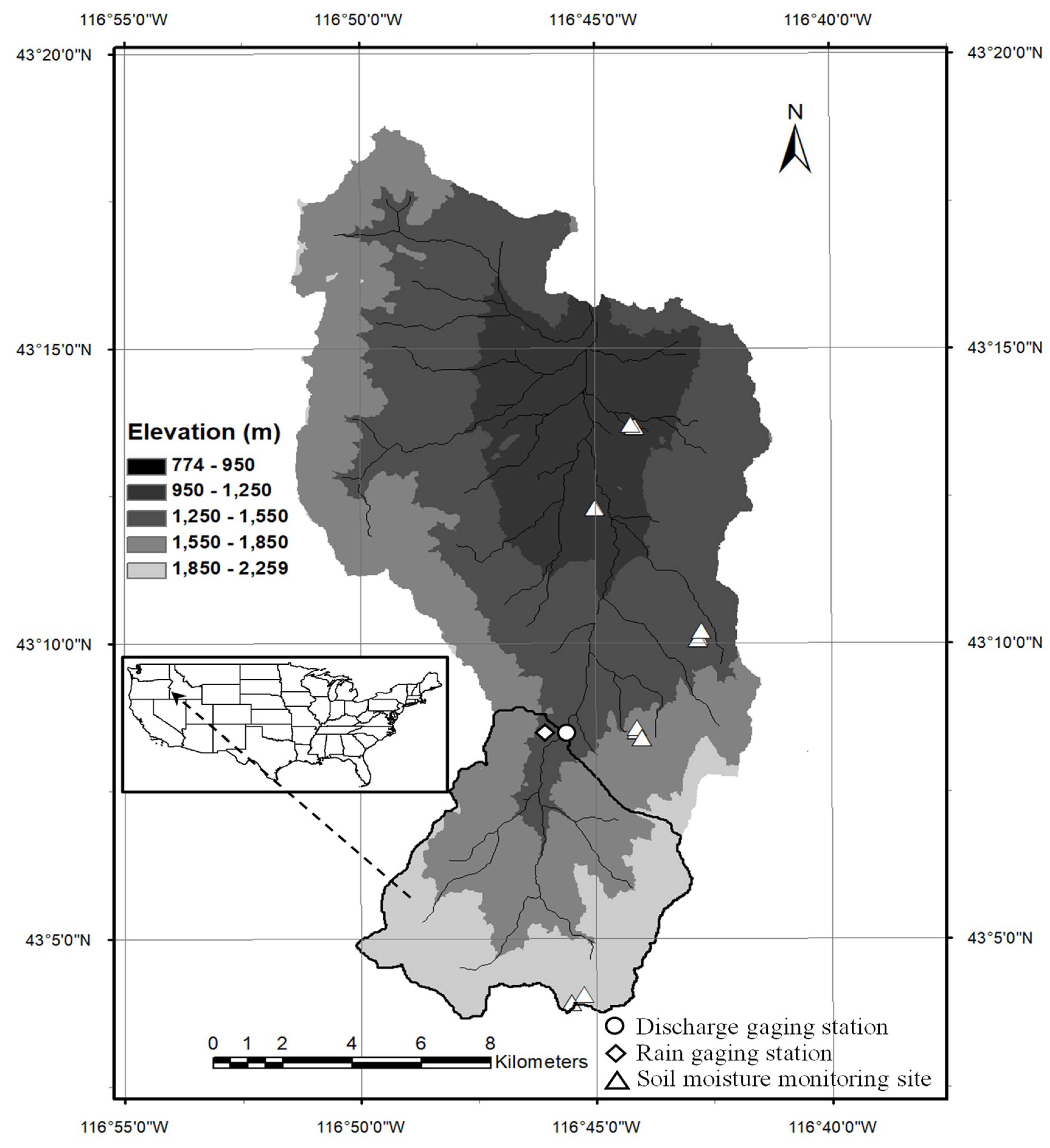
2. Study Area

The Reynolds Creek Experimental Watershed (RCEW), with a catchment area of 239 km² (Figure 1), is located in southwest Idaho and the inter-mountain region of the northwestern USA [34]. The hydrological modelling study area is a 54.7 km² sub-catchment of the RCEW, initiating as the Tollgate weir gaging station No. 116b at 43.142734° N, 116.762493° W WGS84, shown as the round marker in Figure 1. For RCEW, the elevation ranges from 750 to 2100 m a.s.l. with the study sub-catchment above 1400 m a.s.l. Although snow is dominant at the highest elevations, rain generally drives discharge in the RCEW watershed. Precipitation in the RCEW varies from 250 mm/year at lower elevations to more than 1100 mm/year at higher elevations. Land cover in the watershed is dominated by various subspecies of sagebrush, with heights in the range 0.30–0.60 m [35].

3. Data

The observed hourly discharge of Tollgate weir gage was used for calibration and parameter identification of the watershed hydrological model. This discharge data was obtained from the US Department of Agriculture (USDA) Agricultural Research Service (ARS) Northwest Watershed Research Center, ‘reynolds-creek-116b-hourly-streamflow.dat’ retrieved from http://reynoldscreekczo.org/rcewdata/streamflow/reynolds-creek-116b-hourly-streamflow.dat on 1 August 2019. The observed hourly precipitation from rain-gage station No. 116c near Tollgate weir gage was used for hydrological model simulation. This precipitation data was obtained from USDA ARS Northwest Watershed Research Center (2015), ‘reynolds-creek-116b-hourly-streamflow.dat’ retrieved from http://reynoldscreekczo.org/rcewdata/precipitation/reynolds-creek-116c-hourly-precipitation.dat on 1 August 2019. The rain gage station 116c is at 43.141415° N, 116.767242° W WGS84, 1460 m a.s.l.

The land-cover maps for the study area were derived from the National Land Cover Database (NLCD), http://www.mrlc.gov/.

The wilting point (θ_wp) and field capacity (θ_fc), used in the SERVES soil moisture estimation carried out in this study, were derived from the Natural Resources Conservation Service (NRCS) Soil Survey Geographic Database (SSURGO) database, http://websoilsurvey.sc.egov.usda.gov/App/WebSoilSurvey.aspx, using established pedotransfer functions that yield θ_wp and θ_fc as functions of soil texture [36].

The US Geological Survey [37] Earth Resources Observation and Science (EROS) Center Science Processing Architecture (ESPA), https://espa.cr.usgs.gov/, on-demand interface provides 30-m Landsat Surface Reflectance, with atmospheric corrections applied, Level-2 science products that include the spectral indices products for Landsat 4–5 Thematic Mapper (TM), Landsat 7 Enhanced Thematic Mapper Plus (ETM+), and Landsat 8 Operational Land Imager (OLI)/Thermal Infrared Sensor (TIRS). The Normalized Difference Vegetation Index (NDVI), one of the on-demand spectral indices products, was used in the SERVES soil moisture estimation carried out in this study. The USGS Global Visualization Viewer, http://glovis.usgs.gov/, was used to identify the clear-day images in the growing season.

The observed soil moisture data for the June–September growing seasons of 2006–2009, for the moisture measuring stations in the RCEW (Figure 1), were obtained from the public database at Northwest Watershed Research Center, Reynolds Creek Experimental Watershed, Public-use Datafiles and Documentation [35].

4. Methodology

This study analyzed the significance of 30 m hill slope scale, initial soil moisture estimates compared to coarse, 4.5 km and 9 km resolution inputs in calibration, parameterization, and performance of the physics-based distributed hydrological model. The distributed 30 m hill slope scale soil moisture input is derived from the integrated satellite and ground-based SERVES estimates. SERVES soil moisture estimates were compared with in situ measured soil moisture at several locations. Validated estimates were used as distributed initial soil moisture condition in calibration and parameterization of the hydrological model. The simulations were repeated with resampled soil moisture initial condition resolution of 4.5 km and 9 km. The GSSHA model was deployed to drive physics-based distributed watershed hydrological simulations of rainfall and runoff events. The topographic and computational model grid resolution was fixed at 30 m for all the initial soil moisture input scenarios. For all scenarios, the comparison and analysis were performed for consistency of parameterization, discharge output performance, and the resulting distribution of simulated soil moisture state.

4.1. SERVES (Soil Moisture Estimation of Root Zone Through Vegetation Index-Based Evapotranspiration Fraction and Soil Properties) Model Formulation

The relationship between reference evapotranspiration fraction, ET_rf, with soil moisture is defined as [4]:

$${\theta }_i=E{T}_{rfi}({\theta }_{fci}-{\theta }_{wpi})+{\theta }_{wpi}$$

(1)

where,

• θ = soil moisture content;
• θ_fc = field capacity soil moisture content; and
• θ_wp = wilting point soil moisture content;
• i = any spatial location or grid/tin address for a numerical model.

From the parametric uncertainty analysis of the linear deterministic relationships between ETrf and the normalized difference vegetation index, NDVI, the likelihood function of evapotranspiration fraction inversion through NDVI is defined as [4]:

$$E{T}_{rf}=1.33 NDVI-0.049$$

(2)

From Equations (1) and (2), spatially distributed soil moisture content is derived as:

$${\theta }_i=\left(1.33NDVI-0.049\right)({\theta }_{fci}-{\theta }_{wpi})+{\theta }_{wpi}$$

(3)

Pradhan [4] developed Equation (3) as the root-zone soil moisture estimation model SERVES. The details on the development, application and verification of Equation (3) is shown in Pradhan [4].

Root zone soil moisture interacts directly with the atmosphere through evaporation and drives infiltration, hence run off during heavy rain events. Soil moisture data from satellite or remotely sensing platforms has a maximum soil column depth of 10 cm. Root zone soil moisture accounting depth reaches deeper for most of vegetation species. The SERVES method estimates the soil moisture at the root zone depth by taking into account the soil physical properties.

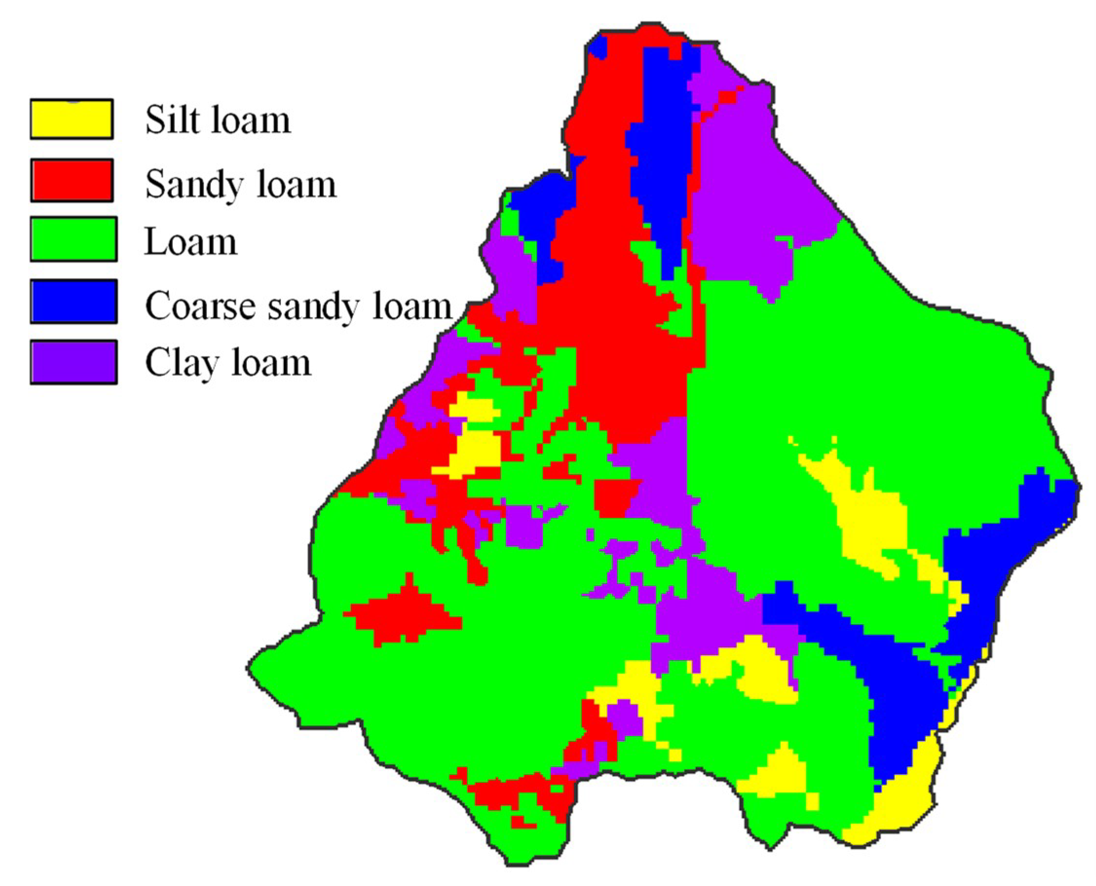
Identification of SERVES Soil Physical Properties

Soil texture is an important factor governing a range of physical properties and processes in soil. There are various sources for soil texture classification. Among these sources, the NRCS, SSURGO provides soil textural information for continental United States at 30-m resolution. LaHatte and Pradhan [38] show a guideline on extracting the soil texture from the SSURGO database.

Once the soil texture is identified, pedotransfer functions estimate soil water properties. Rawls et al. [36] is a common source for soil physical parameter value assignments based on the soil texture, see

Table 1. Soil infiltration parameter values from soil textural classification [36].

Soil Type	Silt Loam	Sandy Loam	Loam	Coarse Sandy Loam	Clay Loam
Saturated hydraulic conductivity (cm/h)	0.199	0.199	0.199	0.199	0.199
Capillary head (cm)	10.5	10.7	10.0	10.7	10.7
Porosity (m3/m3)	0.48	0.41	0.43	0.41	0.39
Pore distribution index (cm/cm)	0.234	0.378	0.252	0.378	0.242
Residual point (m3/m3)	0.015	0.041	0.027	0.041	0.075
Field capacity (m3/m3)	0.33	0.207	0.270	0.207	0.318
Wilting point (m3/m3)	0.133	0.095	0.117	0.095	0.197

.

Figure 2 shows the RCEW study sub-catchment SSURGO soil texture classification identified through the process described in [38]. Table 1 shows the soil infiltration parameter values from soil textural classification [36].

Table 1 shows the soil infiltration parameter values from soil textural classification [36].

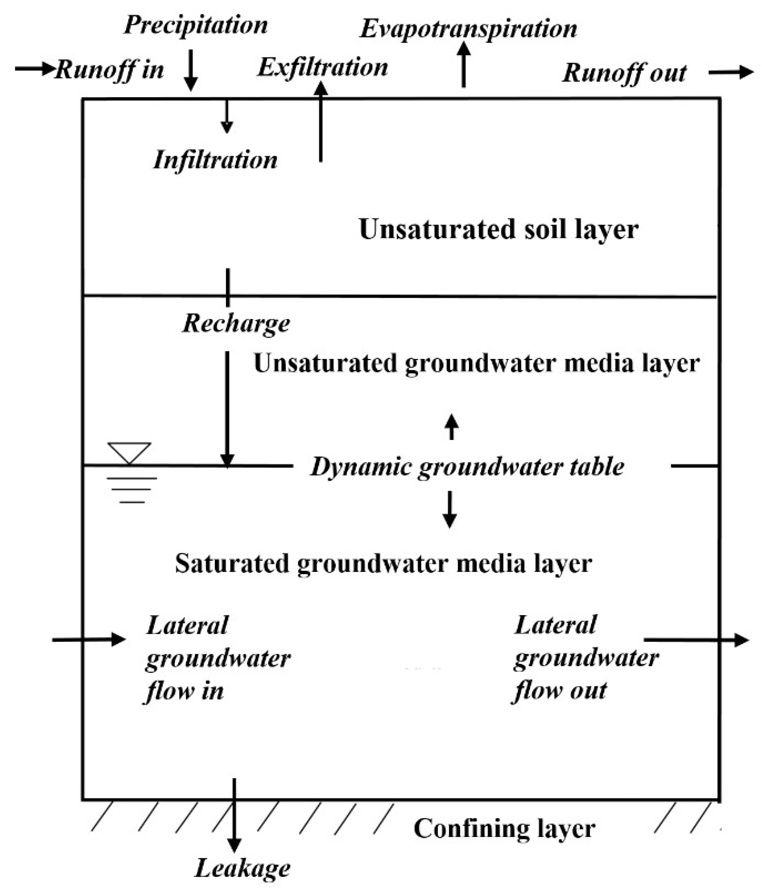
4.2. GSSHA (Gridded Surface Sub-Surface Hydrological Analysis) Model

The GSSHA model was developed to allow simulations of coupled surface-water/groundwater systems. The link between the surface-water zone and the saturated groundwater zone is the area between the two domains, referred to as the unsaturated zone, or the vadose zone. This area controls the important fluxes of infiltration, evapotranspiration (ET), and groundwater recharge. The movement of water in the unsaturated zone is largely vertical [39] and GSSHA was developed with a one-dimensional (1-d) representation of the unsaturated zone.

The 1-d unsaturated vadose zone in this study is represented by two-layer Green and Ampt model [40] with redistribution [41] as shown in Figure 3 to provide estimates of infiltration flux into the unsaturated zone (GSSHAWIKI, 2011, http://www.gsshawiki.com, accessed on 15 December 2019).

Water enters the top layer soil as infiltration, and leaves the layer either as recharge to groundwater or as evapotranspiration to atmosphere. For groundwater recharge from top layer, a unit head gradient is assumed, so that the recharge is equal to the unsaturated hydraulic conductivity as shown by Equation (4) [42].

$$K\left(\theta \right)=K_s{\left(\frac{\theta -{\theta }_r}{{\theta }_s-{\theta }_r}\right)}^{3+2/\lambda }$$

(4)

where

• K(θ) = soil moisture dependent hydraulic conductivity of the soil (m/s);
• K_s = saturated hydraulic conductivity of the soil (m/s);
• θ = water content of the soil;
• θ_s = saturated water content of the soil;
• θ_r = residual water content of the soil; and
• λ = is soil distribution index.

The updated volume of water in the top soil layer is defined by the following mass balance equation:

$$Vo{l}^{n+1}=Vo{l}^n+\Delta t Acell \left(Inf-Rech-AE\right)$$

(5)

where

• Volⁿ⁺¹ = the updated volume of water in the soil layer (m³);
• Volⁿ = the volume of water in the soil layer at the time of the last update (m³);
• Δt = the amount of time that has elapsed since the last updates (s);
• Inf = the infiltration rate (m/s);
• Rech = the groundwater recharge rate (m/s);
• Acell = the surface area of the cell (m²);
• AE = the actual evapotranspiration (m/s).

The soil moisture in each layer of a cell is computed as the updated volume of soil water in the layer divided by the layer depth. The dynamic groundwater table at different layers controls the layer depth and water fluxes to and from the layers. When the groundwater table is at the groundwater unsaturated layer, the volume of water in this zone is considered part of the unsaturated zone water but not as part of the soil layer. Fluxes are added to, or subtracted from, the groundwater to account for the water in the unsaturated portion of the groundwater media as the water table rises and falls, respectively. As the water table continues to rise, the bottom layer is reduced until it disappears. The same process is repeated as the water table rises into the top layer. If only one soil layer is specified, the process is the same. When the water table in the first layer reaches to the soil surface, infiltration into the cell ceases and the groundwater storage term becomes unity. In this case, if the groundwater elevation is higher than the surface-water elevation then groundwater will spill back onto the overland flow plane as exfiltration. There is 2-d saturated groundwater later flow.

5. Results and Discussion

Rainfall event of the year 2014 was taken for the hydrological model simulations. Early fall/late summer rainfall event of 28 September to 29 September 2014 was used for calibrating and parameter identification of the hydrological model. The RCEW long-term observed hydrograph shows that the base flow, ground water contribution, is at the lowest in the fall season. Most of the physics-based hydrological models with base flow capabilities are formulated to take account of shallow groundwater processes that link the vadose zone hydrology to surface runoff, and that makes the base flow sink or source to stream. Similarly, the GSSHA is limited to shallow ground water. Hence to avoid identification of incorrect calibrated parameter values the lowest base flow period, late summer/early fall season’s event, is chosen for the hydrological model analysis.

5.1. SERVES Estimated Initial Soil Moisture

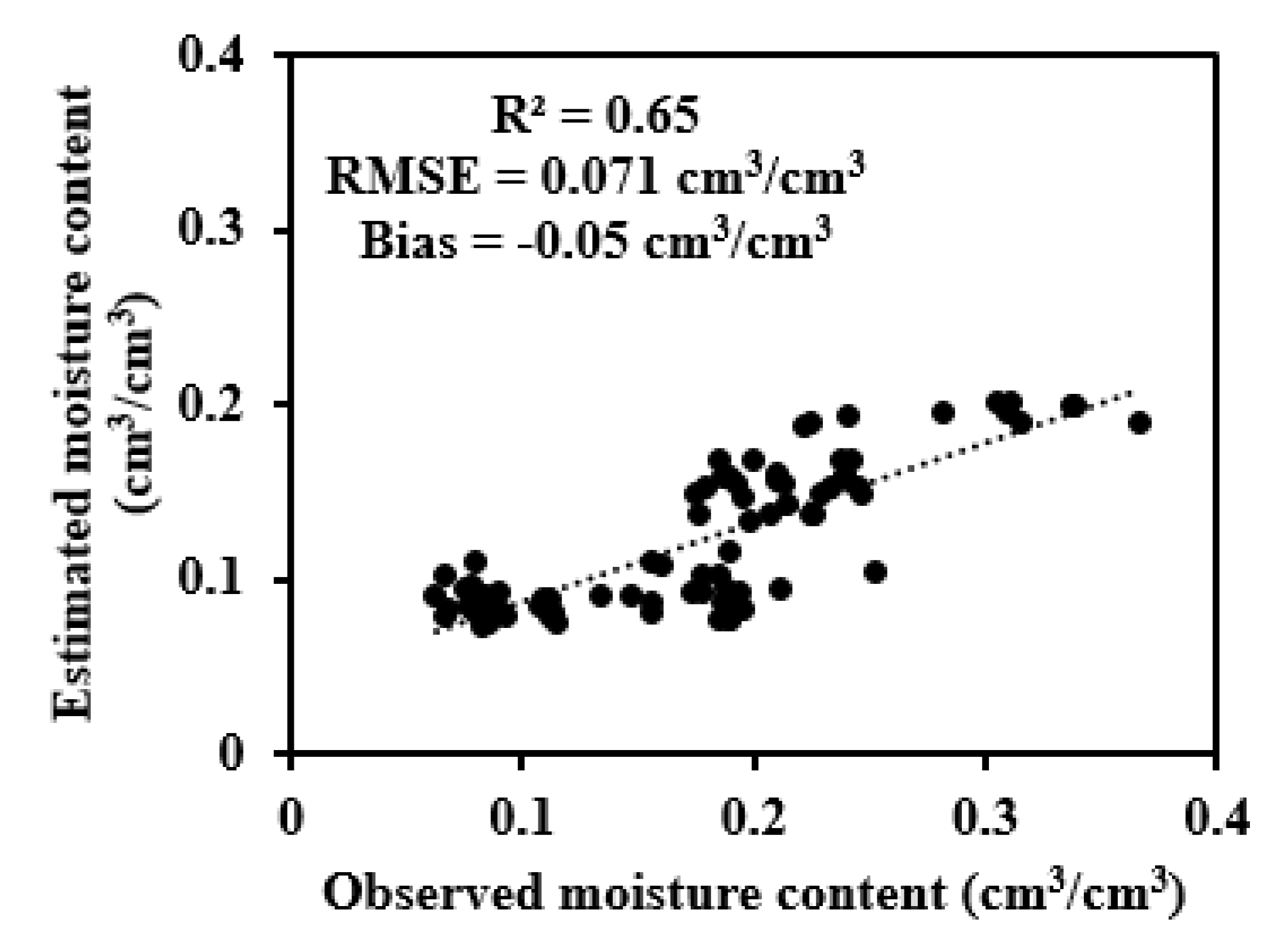
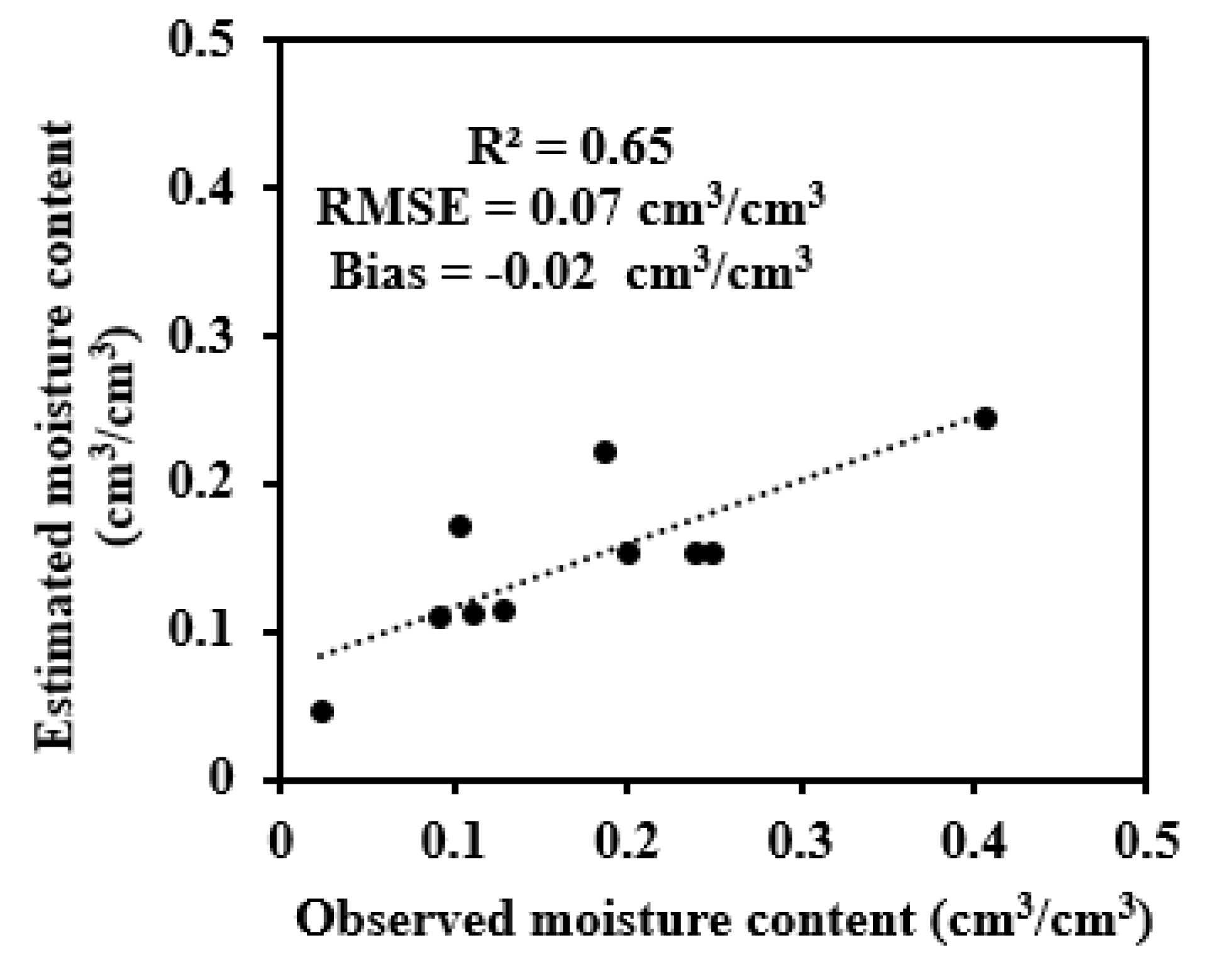
5.1.1. Verification of SERVES Estimated Soil Moisture

Figure 4 shows the comparison of SERVES estimated soil moisture with the in situ soil moisture observed at soil moisture measurement sites in the growing season of the years 2006, 2007, 2008 and 2009 in the RCEW [4]. In Figure 4, the coefficient of determination (R²) was 0.65, the root mean square error (RMSE) was 0.071 cm³/cm³ and bias was −0.05 cm³/cm³. Pradhan [4] also showed successful application of the SERVES method in other regions of northwest United States.

Figure 5 shows the scatter plot of the available observed soil moisture versus SERVES calculated soil moisture in the month of September 2014 for the soil moisture measurement sites in the RCEW as shown in Figure 1. In Figure 5, the coefficient of determination (R²) was 0.65, the root mean square error (RMSE) was 0.07 cm³/cm³ and bias was −0.02 cm³/cm³. September of 2014 is selected in Figure 5 because in this study, RCEW GSSHA model simulation was made for the September rainfall event.

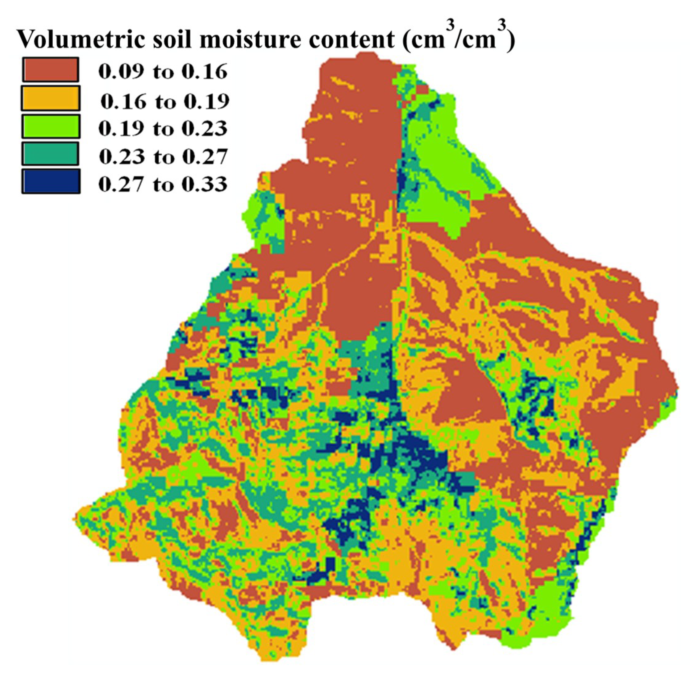
5.1.2. Development of Soil Moisture Initial Condition

A rainfall event of 28 September 2014 was used for the parameter identification and calibration of the hydrologic model calibration. Hence, SERVES soil moisture was estimated with the Landsat vegetation index imageries having the satellite overpass date that was closest to the rainfall event. The θ_wp and θ_fc for the soil type shown in Figure 2 are defined in Table 1. SERVES Equation (3) was used to estimate soil moisture and the estimated soil moisture map is shown in Figure 6.

5.2. Watershed Hydrological Model Development and Parameter Value Identification

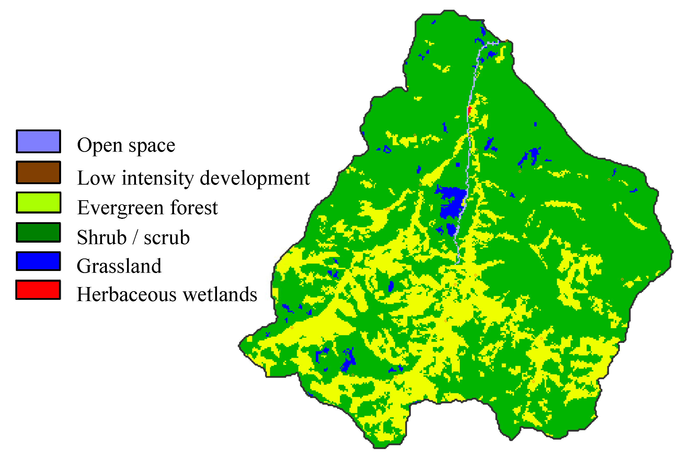
5.2.1. Model Development

The hydrological model was developed with the infiltration and soil moisture accounting processes defined in the methodology section. Pedotransfer functions estimated the soil water properties as defined by Table 1 for the soil texture identified in Figure 2. In Table 1, except for soil hydraulic conductivity, the source for soil physical parameter value assignments was based on [36].

Diffusive wave approach was deployed to route the generated overland runoff. The Manning’s roughness parameter values for the routing model as shown in

Table 2. The Manning’s roughness parameter values for the routing model.

Land Use Type	Manning’s Roughness Value
Open space	0.09
Low intensity development	0.05
Evergreen forest	0.25
Shrub/scrub	0.45
Grassland	0.4
Herbaceous wetlands	0.15

were employed from the literature [43,44]. The land-use types defined in Table 2 are from Figure 4

Two dimensional (2-d) overland flow, 1-d stream flow, 1-d infiltration are fully coupled with 2-d groundwater. In GSSHA, only the surficial aquifer is simulated, so the saturated groundwater domain is down to the first confining layer in the subsurface. The unsaturated zone domain is any soil above the saturated zone. The unsaturated domain is dynamic in both space and time and can vary from no domain (groundwater table is at or above the soil surface) to the depth of the surficial aquifer, depending on groundwater conditions. Higher elevations of the Reynolds Creek Experimental Watershed are underlain by basalt and latite [45]. Soils derived from basalt and latite tend to be deeper, with higher organic matter content and finer texture [45]. Therefore, to account for the deeper unsaturated, saturated groundwater soil horizon, the bedrock in the model is conceptually set at 20 m deep. Flerchinger et al. [46] shows that the observed water table in the subwatershed of RCEW fluctuates tens of meters in a year with maximum level in the summer season and minimum in the fall season. Hence to conceptually allow for increasing limit of the watertable in the summer and also to set a minimum water table level from the confining layer, the groundwater table is set at 2 m above the bed rock and the model was allowed to spin up without rain to equilibrate and settle this water table. The settled water table at the end of the spin up period was then deployed as the initial condition.

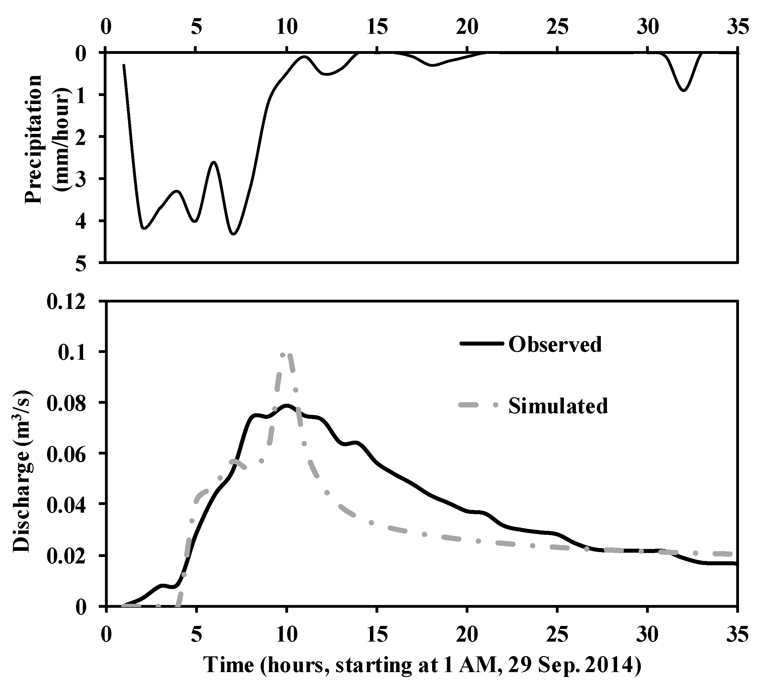
5.2.2. Model Calibration

In previous GSSHA model calibrations [30,31,32,33], parameter values were adjusted manually to achieve an acceptable fit to the observed hydrograph with parameter values bounded by physical understanding and the experience with the model. This study undertook a similar manual calibration approach for the event of 28 September 2014. Hydraulic conductivity in Table 1 was manually calibrated.

Calibration of the distributed GSSHA hydrologic model is greatly simplified by allocating key dominant parameters for calibration and by directly assigning the values for the rest of the parameters based on soil and land-use classification. Such a direct assignment of parameter values require the physical basis of the hydrological processes along with the knowledge and experience of the model.

GSSHA implements Manning’s equation to relate surface roughness to flow rate, in which case the hydraulic roughness is represented by the Manning’s roughness coefficient, n [47]. For each land-use type shown in Figure 7, a Manning’s roughness coefficient was calibrated within the range of physical values. Table 2 lists the calibrated Manning’s roughness coefficients in the study area.

Nash–Sutcliffe efficiency maximization was the objective function in the model performance optimization. The Nash–Sutcliffe efficiency obtained in Figure 8 is 62%.

5.3. Disparity in Parameter Identification Scale and Moisture Initial Condition Application Scale

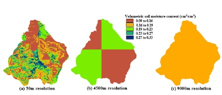
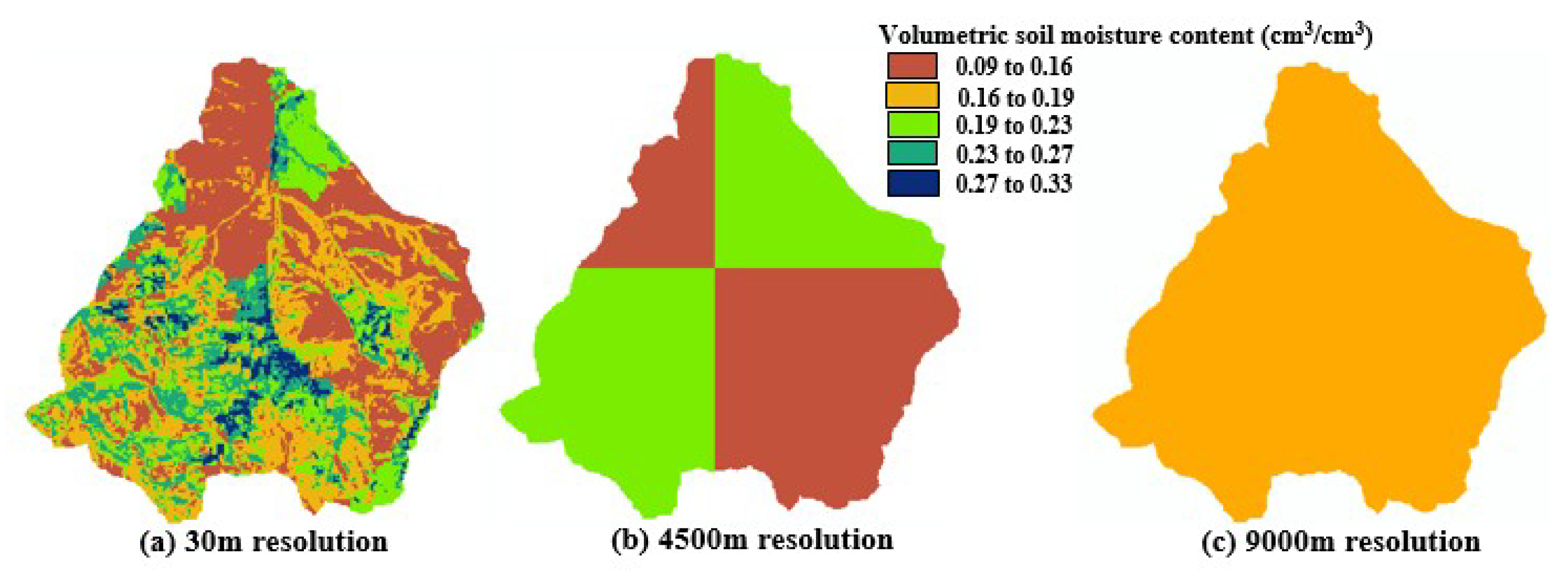
5.3.1. Resampling of Initial Soil Moisture

The 30 m initial soil moisture map shown in Figure 9a is resampled to 4.5 km and 9 km grid resolution as shown in Figure 9b and Figure 9c. From Figure 9 it is clear that resampling into coarser grid resolution, the finer soil moisture information is completely averaged out. The resampled 4.5 km and 9 km grid resolution was divided back to 30 m grid resolution without disaggregating the values and was used individually as initial condition input with the same parameters, Table 1 and Table 2, identified by 30 m resolution initial soil moisture input as shown in calibration Figure 8.

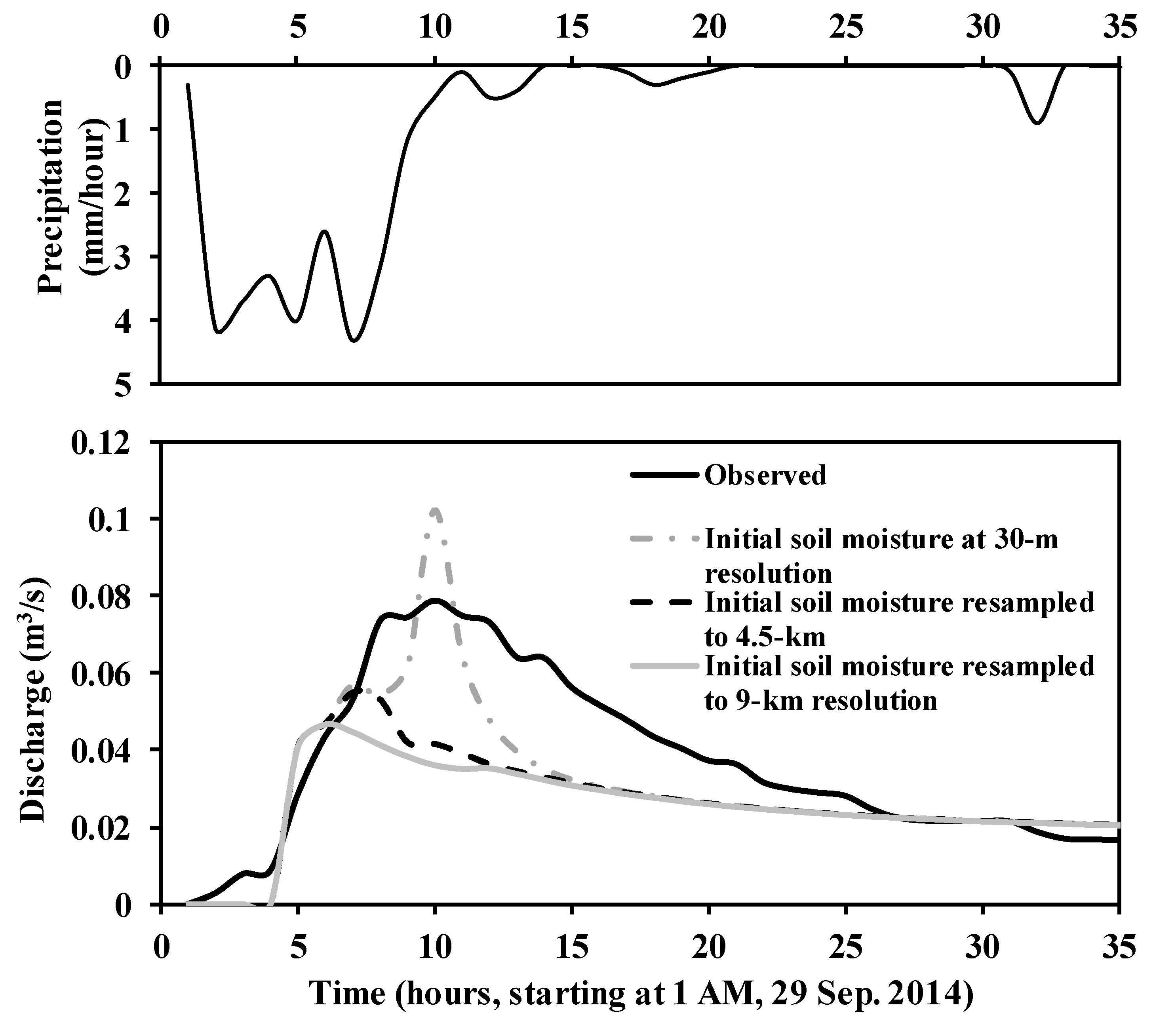
5.3.2. Inconsistency in Simulated Discharge

With the same parameter values identified at 30 m initial soil moisture input resolution and applying the coarser resolution initial soil moisture resulted in significant underestimation in the output simulated discharge as shown in Figure 10. In Figure 10, the Nash–Sutcliffe efficiency for simulated discharge with 4.5 km is 35% and that for 9 km is 25%. This shows that there is inconsistency in model output discharge when the model parameter identification scale of initial soil moisture does not match with the model application scale of initial soil moisture.

5.3.3. Inconsistency in the Parameter Values

Figure 10 shows the inconsistency in the simulated discharges at different initial soil moisture input resolution but with same parameter values identified at finer initial soil moisture input resolution. It was found that the consistency in the simulated discharge can be regained if the parameter values are re-calibrated or identified for the initial moisture resolution. As soil moisture is a state of the soil condition, this study identified that re-calibrating the soil hydraulic conductivity regained consistency in the simulated discharge. The calibrated hydraulic conductivity values decreased by 8.0% and 13%, as shown in

Table 3. Resolution of the initial soil moisture condition and its’ effect on the calibrated soil hydraulic conductivity parameter value.

Soil Moisture Resolution Factor	% Decrease in the Hydraulic Conductivity Calibrated Value
150	8.0
300	13.0

, for 4.5 km and 9 km moisture input resolution respectively in comparison to the calibrated hydraulic conductivity values identified at 30 m moisture input resolution. In Table 3, the resolution factor is the resampled grid resolution, which is 4.5 km and 9 km in this example, to the original soil moisture input resolution, which is 30 m in this example.

Figure 11. shows that the same 62% NS efficiency was obtained when the hydraulic conductivity was decreased as shown in Figure 10.

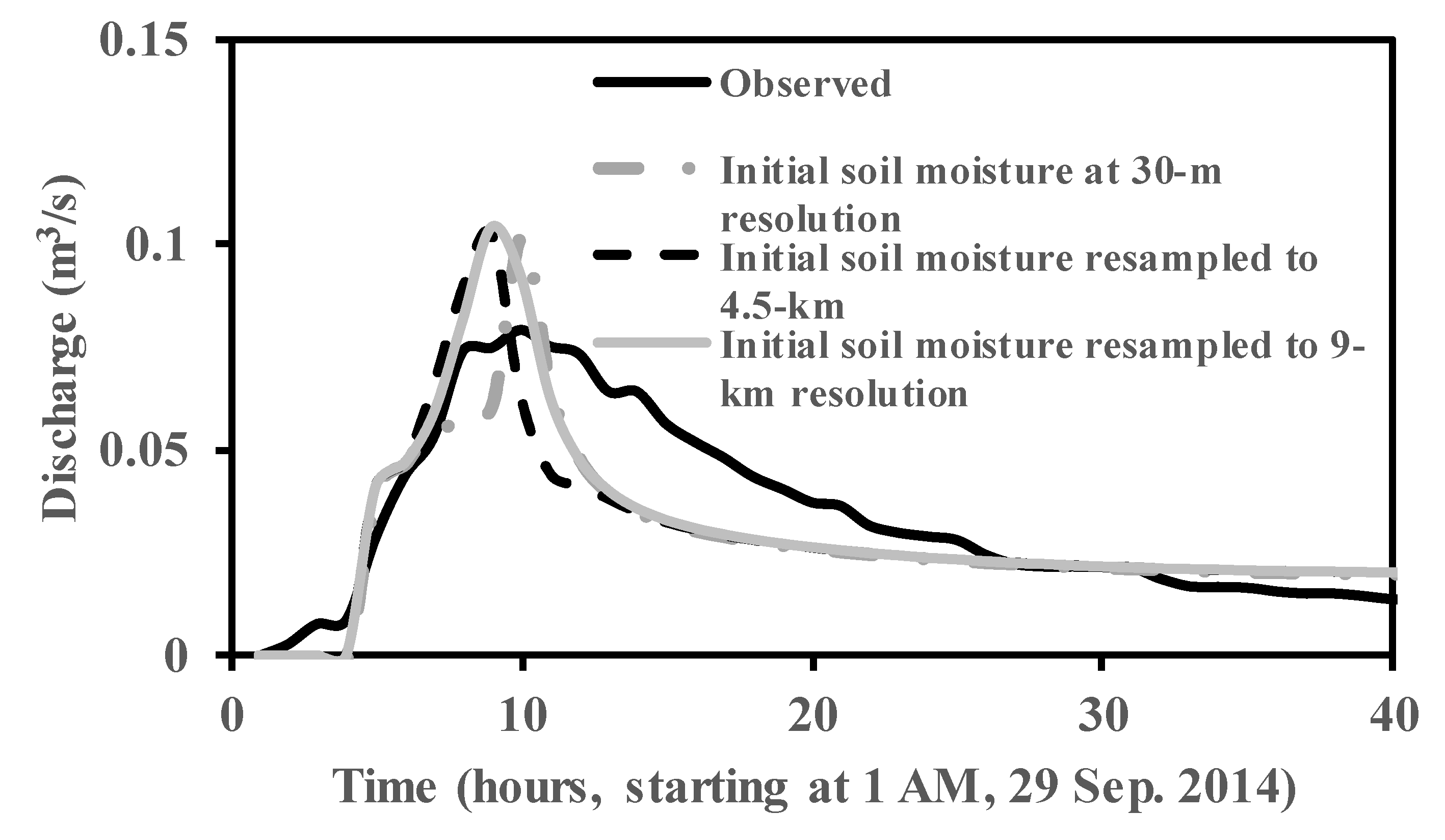
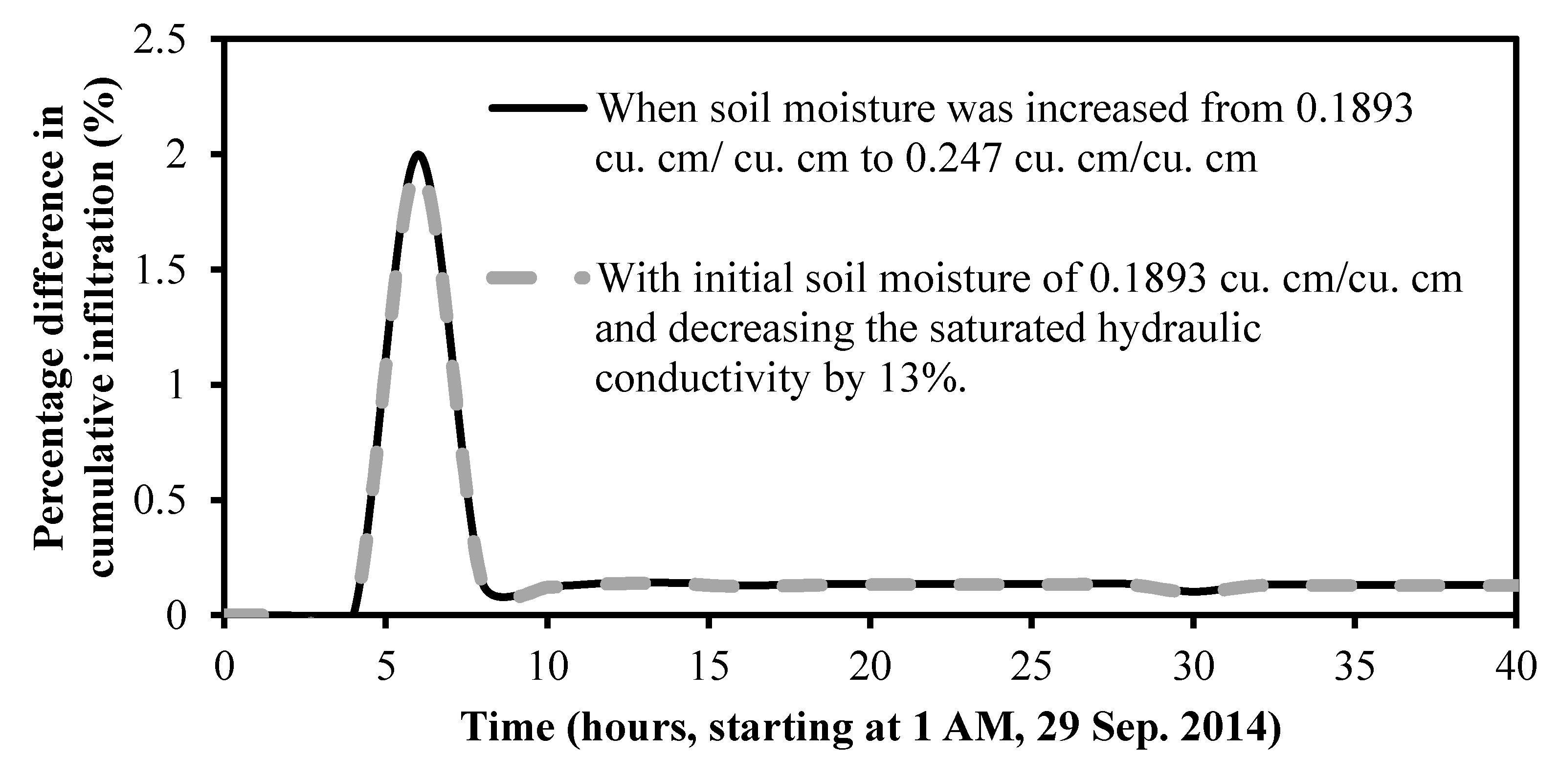
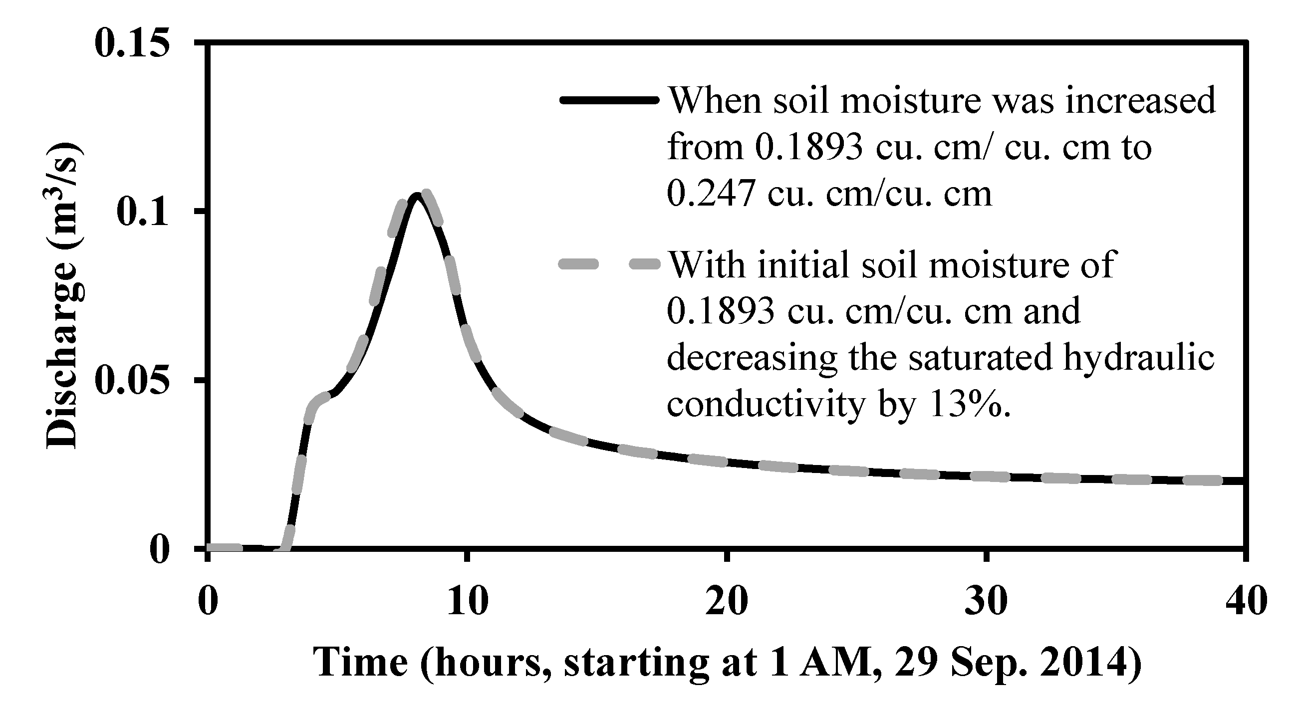
Readjustment of Either Hydraulic Conductivity Value or Soil Moisture Value

In an infiltration process, Green and Ampt-based infiltration in this case, infiltration rate is a function of soil moisture deficit and soil hydraulic conductivity. Increasing soil moisture deficit increases the infiltration. Increasing soil hydraulic conductivity also causes the infiltration rate to increase.

Soil moisture deficit, $\Delta \theta ,$ is defined as:

$$\Delta \theta ={\theta }_s-\theta$$

(6)

where, θ_s is saturated water content of the soil, and θ is the water content of the soil.

Figure 9 shows that higher values of the soil water content is completely filtered out at 9 km initial soil moisture input resolution. The value of this uniform soil moisture in Figure 9c was 0.1893 cm³/cm³. Increasing this uniform soil moisture to 0.247 cm³/cm³ reproduced the simulated discharge with the same 62% Nash–Sutcliffe efficiency. This is because increasing the soil moisture reduced the soil moisture deficit which in turn increased the infiltration rate. Figure 12 shows the difference in the simulated cumulative infiltration with 0.245 cm³/cm³ initial soil moisture and that of 0.1893 cm³/cm³ initial soil moisture.

According to Equation (4), soil hydraulic conductivity is a function of soil moisture content. If soil moisture is lower, the soil hydraulic conductivity decreases. In fact, a decrease in the soil hydraulic conductivity decreases the infiltration rate, as defined by the Green and Ampt infiltration process. But this decrease in the soil hydraulic conductivity in Equation (4) alone could not compensate for the increment in the infiltration rate due to a decrease in the soil moisture value at a coarse resolution, 9 km. In this case, it was found that, to compensate for the increase in the infiltration rate due to coarser initial soil moisture input resolution, the saturated hydraulic conductivity needed to decrease. Therefore, the difference of the cumulative infiltration rate with and without the 13% decrease in the saturated hydraulic conductivity for 0.1893 cm³/cm³ initial soil moisture at 9 km resolution, in Table 3, produced the similar cumulative infiltration difference with 0.245 cm³/cm³ initial soil moisture and that of 0.1893 cm³/cm³. This makes it clear that to achieve scale invariant discharge from a coarser resolution initial soil moisture input resolution, 9 km in this case, either the initial soil moisture value needs to be increased or the saturated hydraulic conductivity needs to be decreased. Figure 13 shows that the 62% Nash–Sutcliffe efficiency in the simulated hydrograph was achieved with either 13% decrease in the saturated soil hydraulic conductivity or with readjustment of the soil moisture from 0.1893 cm³/cm³ to 0.247 cm³/cm³.

Although there are various sources and resolutions of remotely sensed soil moisture data, the analysis in this section provides an option on how to compensate the effect of disparity in the parameter value identification scale of the initial soil moisture and the parameter value application scale of the initial soil moisture.

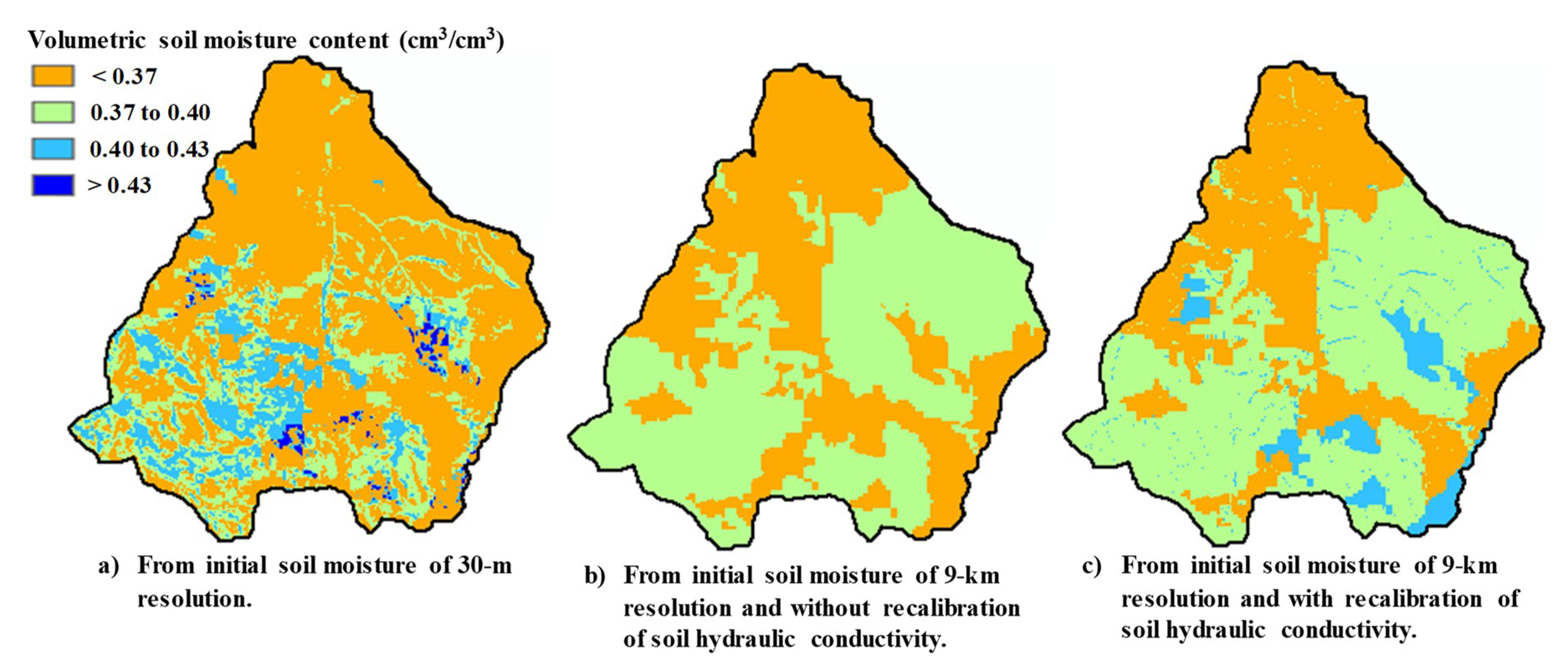
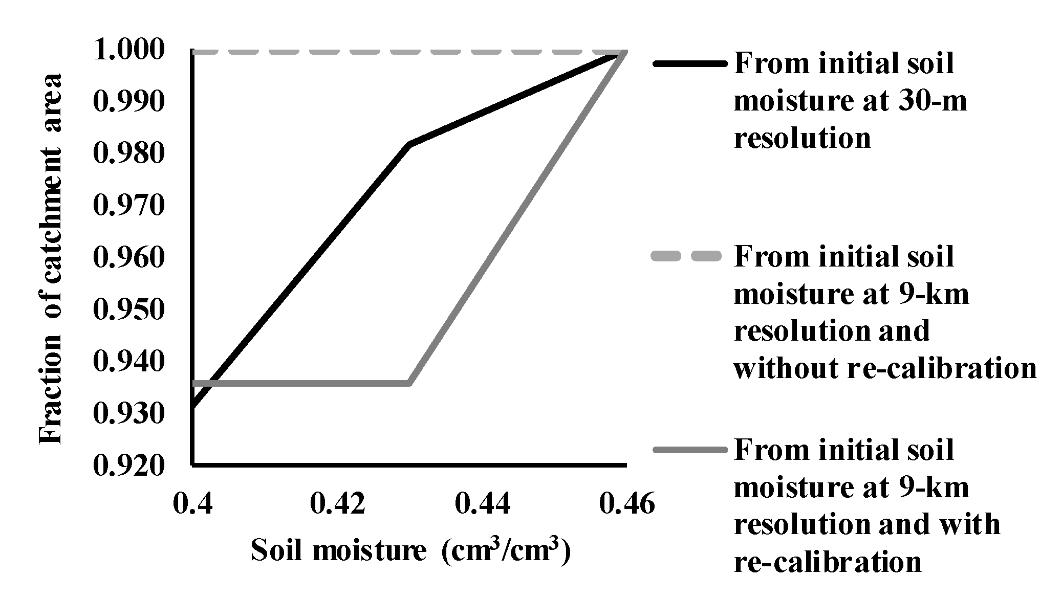
5.3.4. Inconsistency in the Distribution of Simulated Soil Moisture State

As shown in Figure 11, changing the parameter values of the soil hydraulic conductivity corrected the simulated discharge. The analysis was extended to determine the resolution effect of initial soil moisture condition on the simulated soil moisture state as shown in Figure 14 and Figure 15. Further research was undertaken to see the effect of the readjustment of the soil hydraulic conductivity, for correcting the simulated discharge, in the simulated soil moisture state as shown in Figure 14 and Figure 15.

Figure 14 and Figure 15 show the comparison of the simulated soil moisture state from 30 m and 9 km—available satellite-based digital soil moisture data are at a resolution of 9 km and above—with the initial soil moisture condition.

Figure 14a is the soil moisture state at the peak of the event of Figure 11 obtained from the hydrologic model simulation from 30 m resolution initial soil moisture condition. Figure 14b is the soil moisture state at the peak of the event of Figure 11 obtained from the hydrologic model simulation from 9 km resolution initial soil moisture condition and with the same hydrological model parameter values as that in Figure 14a. Figure 14b shows the soil moisture of higher values is filtered out in comparison to that in Figure 14a. In Figure 15, the solid black line represents the cumulative soil moisture distribution of Figure 14a and the grey dotted line represents the cumulative soil moisture distribution of Figure 14b. The comparison of these cumulative distributions makes it clear that the higher values of the simulated soil moisture state is filtered out when coarser resolution soil moisture initial condition is applied.

Figure 14c and the solid grey line in Figure 15 is the simulated soil moisture after adjusting the soil hydraulic conductivity to correct the discharge simulation as shown by the solid grey line in Figure 11. It is clear the readjustment of the soil hydraulic conductivity in Figure 14c and Figure 15 helped to regenerate the filtered higher valued soil moisture state. This regeneration of the filtered soil moisture value, especially when directly applying coarse resolution satellite soil moisture data, by readjustment of the hydrological model soil parameter, soil hydraulic conductivity, could be an indirect soil moisture state scaling approach. The term indirect is employed because of the fact that the scaling in the soil moisture state is undertaken through the adjustment of the model parameters.

6. Conclusions

Impacts such as those due to climate change cross multiple spatial scales from local to regional to global. Hydrological studies for planning, design and construction under such impacts also cross multiple spatial scales from local to regional to global. Therefore, a single high-resolution soil moisture input is not always feasible for a large-scale hydrological analysis. This study evaluated effective root zone soil moisture input data resolution effects on the consistency of physics-based, distributed hydrological model infiltration parameterization and simulation results. Satellite-based SERVES 30 m hill-slope scale resolution soil moisture estimates were used for calibration of the distributed hydrological model. As the initial soil moisture was resampled to 4.5 km and then to 9 km resolution, the hill-slope soil moisture variability was lost due to spatial averaging. Ultimately, this averaging resulted in a lower effective value of the initial root zone soil moisture. Model calibration, parameter identification, and simulation performance of the physics-based distributed hydrological model was made with hill-slope scale, 30 m resolution, initial soil moisture condition. The simulations were repeated with resampled soil moisture initial condition resolutions of 4.5 km and 9 km. The GSSHA model was deployed to drive physics-based distributed watershed hydrological simulations of rainfall and runoff events in which the topographic and computational model grid resolution was fixed at 30 m for all of the initial soil moisture input scenarios. For all of the initial soil moisture input resolution scenarios, the comparison and analysis were performed for the consistency of the parameter identified values, the discharge output performance, and the distribution of the hydrological model simulated distributed soil moisture state. It was found that by changing the input resolution of the initial soil moisture condition to coarser grid scale would produce significantly underestimated discharge and overestimated infiltration rate/volume with filtered out higher soil moisture state distribution when simulated with hydrological model parameters calibrated/identified at finer resolution initial soil moisture resolution. The inconsistency and underestimation in the simulated discharge, due to application of the coarse-resolution soil moisture initial condition, was recovered by recalibration of the model that decreased the soil hydraulic conductivity parameter value. The recalibration/readjustment of the soil hydraulic conductivity value was found to compensate for the inconsistency in the simulated discharge and infiltration rate and regenerate the filtered out higher soil moisture state distribution.

References

- Berg, A.; Lintner, B.; Findell, K.; Giannini, A. Soil moisture influence on seasonality and large-scale circulation in simulations of the West African Monsoon. J. Clim. 2017, 30, 2295–2317. [Google Scholar] [CrossRef]
- Kang, Y.; Khan, S.; Ma, X. Climate change impacts on crop yield, crop water productivity and food security—A review. Prog. Nat. Sci. 2009, 19, 1665–1674. [Google Scholar] [CrossRef]
- Mananze, S.; Pôças, I.; Cunha, M. Agricultural drought monitoring based on soil moisture derived from the optical trapezoid model in Mozambique. J. Appl. Remote Sens. 2019, 13, 024519. [Google Scholar] [CrossRef]
- Pradhan, N. Estimating growing-season root zone soil moisture from vegetation index-based evapotranspiration fraction and soil properties in the Northwest Mountain region, USA. Hydrol. Sci. J. 2019, 64, 771–788. [Google Scholar] [CrossRef]
- Parajka, J.; Naeimi, V.; Blöschl, G.; Wagner, W.; Merz, R.; Scipal, K. Assimilating scatterometer soil moisture data into conceptual hydrologic models at the regional scale. Hydrol. Earth Syst. Sci. 2006, 10, 353–368. [Google Scholar] [CrossRef]
- Silvestro, F.; Gabellani, S.; Rudari, R.; Delogu, F.; Laiolo, P.; Boni, G. Uncertainty reduction and parameter estimation of a distributed hydrological model with ground and remote-sensing data. Hydrol. Earth Syst. Sci. 2015, 19, 1727–1751. [Google Scholar] [CrossRef]
- Sutanudjaja, E.H.; van Beek, L.P.H.; de Jong, S.M.; van Geer, F.C.; Bierkens, M.F.P. Calibrating a large-extent highresolution coupled groundwater-land surface model using soil moisture and discharge data. Water Resour. Res. 2014, 50, 687–705. [Google Scholar] [CrossRef]
- Wanders, N.; Bierkens, M.F.P.; Jong, S.M.; Roo, A.; Karssenberg, D. The benefits of using remotely sensed soil moisture in parameter identification of large-scale hydrological models. Water Resour. Res. 2014, 50, 6874–6891. [Google Scholar] [CrossRef]
- Pradhan, N.R.; Ogden, F.L. Development of a one-parameter variable source area runoff model for ungauged basins. Adv. Water Resour. 2010, 33, 572–584. [Google Scholar] [CrossRef]
- Western, A.W.; Grayson, R.B.; Green, T.R. The Tarrawarra project: High resolution spatial measurement, modeling and analysis of soil moisture and hydrological response. Hydrol. Process. 1999, 13, 633–652. [Google Scholar] [CrossRef]
- Kerr, Y.; Waldteufel, P.; Richaume, P.; Wigneron, J.P.; Ferrazzoli, P.; Mahmoodi, A.; Al Bitar, A.; Cabot, F.; Gruhier, C.; Juglea, S.E.; et al. The SMOS soil moisture retrieval algorithm. IEEE Trans. Geosci. Remote Sens. 2012, 50, 1384–1403. [Google Scholar] [CrossRef]
- Naeimi, V.; Scipal, K.; Bartalis, Z.; Hasenauer, S.; Wagner, W. An improved soil moisture retrieval algorithm for ERS and METOP scatterometer observations. IEEE Trans. Geosci. Remote Sens. 2009, 47, 1999–2013. [Google Scholar] [CrossRef]
- Pan, M.; Sahoo, A.K.; Wood, E.F. Improving soil moisture retrievals from a physically-based radiative transfer model. Remote Sens. Environ. 2014, 140, 130–140. [Google Scholar] [CrossRef]
- Yueh, S.; O’Neill, P.E.; Kellogg, K.H.; Allen, A.; Bindlish, R.; Brown, M.; Chan, S.; Colliander, A.; Crow, W.T.; Das, N.; et al. SMAP Handbook—Soil Moisture Active Passive: Mapping Soil Moisture and Freeze/Thaw from Space; JPL Publication: Pasadena, CA, USA, 2014; 180p. [Google Scholar]
- López-Vicente, M.; Álvarez, S. Influence of DEM resolution on modelling hydrological connectivity in a complex agricultural catchment with woody crops. Earth Surf. Process. Landf. 2018, 43, 1403–1415. [Google Scholar] [CrossRef]
- Pradhan, N.R.; Tachikawa, Y.; Takara, K. A downscaling method of topographic index distribution for matching the scales of model application and parameter identification. Hydrol. Process. 2006, 20, 1385–1405. [Google Scholar] [CrossRef]
- Pradhan, N.R.; Tachikawa, Y.; Takara, K. Downscaling methods of flow variables for scale invariant routing model. Annu. J. Hydraul. Eng. Jpn. Soc. Civ. Eng.-JSCE 2006, 50, 109–114. [Google Scholar] [CrossRef][Green Version]
- Pradhan, N.R.; Ogden, F.L.; Tachikawa, Y.; Takara, K. Scaling of slope, upslope area and soil water deficit: Implications for transferability and regionalization in topographic index modeling. Water Resour. Res. 2008, 44, W12421. [Google Scholar] [CrossRef]
- Tan, M.L.; Ficklin, D.L.; Dixon, B.; Ibrahim, A.L.; Yusop, Z.; Chaplot, V. Impacts of DEM resolution, source, and resampling technique on SWAT-simulated streamflow. Appl. Geogr. 2015, 63, 357–368. [Google Scholar] [CrossRef]
- Zhang, J.X.; Wu, J.Q.; Elliot, W.J.; Dun, S.; Chang, K.-T. Effects of DEM Resolution on WEPP Hydrologic and Erosion Prediction: A Case Study of Two Forest Watersheds in Northern Idaho. Trans. ASABE 2009, 52, 447–457. [Google Scholar] [CrossRef]
- Fu, S.; Sonnenborg, T.O.; Jensen, K.H.; He, X. Impact of precipitation spatial resolution on the hydrological response of an integrated distributed water resources model. Vadose Zone J. 2011, 10, 25–36. [Google Scholar] [CrossRef]
- Koren, V.I.; Finnerty, B.D.; Schaake, J.C.; Smith, M.B.; Seo, D.J.; Duan, Q.Y. Scale dependencies of hydrologic models to spatial variability of precipitation. J. Hydrol. 1999, 217, 285–302. [Google Scholar] [CrossRef]
- Ogden, F.L.; Julien, P.Y. Runoff model sensitivity to radar rainfall resolution. J. Hydrol. 1994, 158, 1–18. [Google Scholar] [CrossRef]
- Gao, Q.; Zribi, M.; Escorihuela, M.J.; Baghdadi, N. Synergetic use of Sentinel-1 and Sentinel-2 data for soil moisture mapping at 100 m resolution. Sensors 2017, 17, 1966. [Google Scholar] [CrossRef] [PubMed]
- El Hajj, M.; Baghdadi, N.; Zribi, M.; Bazzi, H. Synergic Use of Sentinel-1 and Sentinel-2 Images for Operational Soil Moisture Mapping at High Spatial Resolution over Agricultural Areas. Remote Sens. 2017, 9, 1292. [Google Scholar] [CrossRef]
- Bauer-Marschallinger, B.; Freeman, V.; Cao, S.; Paulik, C.; Schaufle, S.; Stachl, T.; Modanesi, S.; Massari, C.; Ciabatta, L.; Brocca, L.; et al. Toward global soil moisture monitoring with Sentinel-1: Harnessing assets and overcoming obstacles. IEEE Trans. Geosci. Remote Sens. 2019, 57, 520–539. [Google Scholar] [CrossRef]
- Zribi, M.; Gorrab, A.; Baghdadi, N.; Lili-Chabaane, Z.; Mougenot, B. Influence of radar frequency on the relationship between bare surface soil moisture vertical profile and radar backscatter. IEEE Geosci. Remote Sens. Lett. 2013, 11, 848–852. [Google Scholar] [CrossRef]
- USDA (US Department of Agriculture). National Engineering Handbook; Irrigation Guide, Natural Resources Conservation Service; USDA: Washington, DC, USA, 1997; part 652.
- Downer, C.W.; Ogden, F.L. Gridded Surface Subsurface Hydrologic Analysis (GSSHA) User’s Manual, Version 1.43 for Watershed Modeling System 6.1; ERDC/CHL SR-06-1; System Wide Water Resources Program, Coastal and Hydraulics Laboratory, U.S. Army Corps of Engineers, Engineer Research and Development Center: Vicksburg, MS, USA, 2006; 207p. [Google Scholar]
- Ogden, F.L.; Pradhan, N.R.; Downer, C.W.; Zahner, J.A. Relative importance of impervious area, drainage density, width function and subsurface storm drainage on flood runoff from an urbanized catchment. Water Resour. Res. 2011, 47, 2011. [Google Scholar] [CrossRef]
- Pradhan, N.R.; Downer, C.W.; Johnson, B.E. A Physics Based Hydrologic Modeling Approach to Simulate Non-point Source Pollution for the Purposes of Calculating TMDLs and Designing Abatement Measures. In Practical Aspects of Computational Chemistry III; Springer: Berlin, Germany, 2014; pp. 249–282. [Google Scholar]
- Pradhan, N.R.; Loney, D. An analysis of the unit hydrograph peaking factor: A case study in Goose Creek Watershed, Virginia. J. Hydrol. Reg. Stud. 2018, 15, 31–48. [Google Scholar] [CrossRef]
- Pradhan, N.R.; Downer, C.; Marchinko, S. Catchment Hydrological Modeling with Soil Thermal Dynamics during Seasonal Freeze-Thaw Cycles. Water 2019, 11, 116. [Google Scholar] [CrossRef]
- Slaughter, C.; Marks, D.; Flerchinger, G.N.; van Vactor, S.S.; Burgess, M. Thirty-five years of research data collection at the Reynolds Creek Experimental Watershed, Idaho, United States. Water Resour. Res. 2001, 37, 2819–2823. [Google Scholar] [CrossRef]
- Seyfried, M.; Harris, R.C.; Marks, D.G.; Jacob, B. A Geographic Data-Base for Watershed Research, Reynolds Creek Experimental Water-Shed; Technical Bulletin NWRC 2000-3; Northwest Watershed Research Center, US Department of Agriculture, Agricultural Research Service: Boise, ID, USA, 2000.
- Rawls, W.J.; Brakensiek, D.L.; Miller, N. Green-Ampt infiltration parameters from soils data. J. Hydraul. Eng. 1983, 109, 62–70. [Google Scholar] [CrossRef]
- USGS (US Geological Survey). Product Guide, Landsat Surface Reflectance Derived Spectral Indices; Version 3.6; Department of the Interior: Washington, DC, USA, 2017. [Google Scholar]
- LaHatte, W.C.; Pradhan, N.R. Analysis of SURRGO Data and Obtaining Soil Texture Classifications for Simulating Hydrologic Processes; ERDC/CHL CHETN-X-3; U.S. Army Engineer Research and Development Center: Vicksburg, MS, USA, 2016. [Google Scholar]
- Refsgard, J.C.; Storm, B. MIKE SHE. In Computer Models of Watershed Hydrology; Singh, V.P., Ed.; Water Resources Publications: Highlands Ranch, CO, USA, 1995. [Google Scholar]
- Green, W.H.; Ampt, G.A. Studies of soil physics: 1. Flow of air and water through soils. J. Agric. Sci. 1911, 4, 1–24. [Google Scholar]
- Ogden, F.L.; Saghafian, B. Green and Ampt Infiltration with redistribution. ASCE J. Irrig. Drain Eng. 1997, 123, 386–393. [Google Scholar] [CrossRef]
- Brooks, R.H.; Corey, A.T. Hydraulic Properties of Porous Media; hydrology paper 3; Colorado State University: Fort Collins, CO, USA, 1964. [Google Scholar]
- Engman, E.T. Roughness coefficients for routing surface runoff. J. Irrig. Drain. Eng. 1986, 112, 39–53. [Google Scholar] [CrossRef]
- Senarath, S.U.S.; Ogden, F.L.; Downer, C.W.; Sharif, H.O. On the calibration and verification of two-dimensional, distributed, Hortonian, continuous watershed models. Water Resour. Res. 2000, 36, 1495–1510. [Google Scholar] [CrossRef]
- Graham, C.B.; Barnard, H.R.; Kavanagh, K.L.; McNamara, J.P. Catchment scale controls temporal connection of transpiration and diel fluctuations in streamflow. Hydrol. Proces. 2012. [Google Scholar] [CrossRef]
- Flerchinger, G.N.; Deng, Y.; Cooley, K.R. Groundwater response to snowmelt in a mountainous watershed: Testing of conceptual model. J. Hydrol. 1993, 152, 201–214. [Google Scholar] [CrossRef]
- Manning, R. On the flow of water in open channels and pipes. Trans. Inst. Civ. Eng. Irel. 1891, 20, 161–207. [Google Scholar]