Comparison of Different Cropland Classification Methods under Diversified Agroecological Conditions in the Zambezi River Basin

Abstract

Having updated knowledge of cropland extent is essential for crop monitoring and food security early warning. Previous research has proposed different methods and adopted various datasets for mapping cropland areas at regional to global scales. However, most approaches did not consider the characteristics of farming systems and apply the same classification method in different agroecological zones (AEZs). Furthermore, the acquisition of in situ samples for classification training remains challenging. To address these knowledge gaps and challenges, this study applied a zone-specific classification by comparing four classifiers (random forest, the support vector machine (SVM), the classification and regression tree (CART) and minimum distance) for cropland mapping over four different AEZs in the Zambezi River basin (ZRB). Landsat-8 and Sentinel-2 data and derived indices were used and synthesized to generate thirty-five layers for classification on the Google Earth Engine platform. Training samples were derived from three existing landcover datasets to minimize the cost of sample acquisitions over the large area. The final cropland map was generated at a 10 m resolution. The performance of the four classifiers and the viability of training samples were analysed. All classifiers presented higher accuracy in cool AEZs than in warm AEZs, which may be attributed to field size and lower confusion between cropland and grassland classes. This indicates that agricultural landscape may impact classification results regardless of the classifiers. Random forest was found to be the most stable and accurate classifier across different agricultural systems, with an overall accuracy of 84% and a kappa coefficient of 0.67. Samples extracted over the full agreement areas among existing datasets reduced uncertainty and provided reliable calibration sets as a replacement of costly in situ measurements. The methodology proposed by this study can be used to generate periodical high-resolution cropland maps in ZRB, which is helpful for the analysis of cropland extension and abandonment as well as intensity changes in response to the escalating population and food insecurity.

1. Introduction

Croplands are changing continuously and intensively at regional to global scales due to climate change and human activities [1]. Cropland extent is an essential part of crop monitoring because it is fundamental for the analysis of crop inventory and the assessment of crop status [2,3,4,5].

Approximately 90% of staple food production in sub-Saharan Africa is provided by rainfed farming systems [6]. In the Zambezi River Basin (ZRB), variations in climate conditions have a direct influence on crop outputs as they may turn into extreme rainfall or extended period of drought [6,7]. The effects of climate change [8] combined with filed sizes and cropping systems in the basin, contribute to the reduced food production [9]. The reduced food production makes the ZRB one of the most vulnerable regions in terms of food security in the continent. The expansion of cropland is a primary way to increase crop production in sub-Saharan Africa. According to official statistics, the cropland in the ZRB has experienced a considerable increase since the 1980s [10]. The driving force in the rise was due to a major political and socio-economic transition which changed the agricultural landscape, cropping practices, and productivity, and ultimately influenced the water cycle, water resources, and energy generation. Accurate and timely analysis of cropland extent can provide objective information for decision-making in agricultural management, food security early warning, and food allocation in this region. Nevertheless, mapping cropland extent remains challenging in the ZRB, mainly because of landscape heterogeneity, fragmented agricultural fields, and different cropping patterns [8,11,12], which makes it difficult to discriminate cropland from other vegetation classes such as grassland. To avoid these problems, different aspects, including the quality of input data, methodology to be applied and land features, should be considered [13,14,15].

Various approaches have been developed and tested by researchers to obtain an accurate and timely cropland extent. Compared to conventional methods such as field surveys, remote sensing-based cropland identification is a more rapid and cost-effective method [13,14,15], and therefore provides more frequently updated cropland information [15,16,17]. Numerous studies have utilized supervised classification methodologies for cropland mapping using various satellite datasets [1,18,19,20,21]. Among those supervised classifiers, the random forest classifier [18,21], the classification and regression tree (CART), the support vector machine (SVM) [20,22], maximum likelihood and minimum distance [23] and the naive Bayes classifier [24] are commonly used [18]. Based on these approaches, several fine resolution landcover and cropland products have become available in recent years, including the fine resolution observation and monitoring of global land cover (FROM-GLC) dataset at 30 m resolution for 2010 [25], the Landsat-derived GLOBELAND30 (GLC30) dataset at 30 m resolution for 2000 and 2010 [26], the Copernicus global land operations (CGLS) land cover product of Africa (CGLS-LC100 at a 100 m resolution for 2015), the European Space Agency Climate Change Initiative Land Cover, Global Land Cover map at 300 m for 2015 (ESACCL-LC-L4-300), the Sentinel-2 Prototype (ESACCI-LC_S2_Prototype) map for Africa at a 20 m resolution for 2016 [27], and the Global Food Security support analysis data over the continent of Africa for 2015 at a 30 m resolution (GFSAD30AFCE) [18]. The accuracies of these landcover products depend on their input data sources.

Recently, researches evaluated the accuracy of these datasets, and it was found that the GLOBELAND30 (GLC30) had an overall accuracy of 78.6% for the year 2000 and 80% for the year 2010 [26]. The overall accuracy of the ESACCI-LC_S2_Prototype dataset was approximately 65% [27], while ESACCL-LC-L4-300 had an overall accuracy of 71.5% [28]. GFSAD30AFCE [18], FROM-GLC [25], and CGLS-LC100 [29] have as overall accuracies of 94.5%, 64.9% and 74.3%, respectively. Independent validation shows that the overall accuracies of all four datasets (CGLS-LC100 [29], ESACCL-LC-L4-300 [28], GFSAD30AFCE [18], and ESACCI-LC_S2_Prototype [27]) were below 65% [12]. Furthermore, results revealed an overestimation of crop area in most countries when compared with the statistics from the Food and Agriculture Organization (FAO) [30]. Several studies have attempted to include more indicative spectral features to improve classification accuracy [5,18]. For example, taking advantage of crop growth features derived from satellite data, the GFSAD30AFCE obtained a relatively higher accuracy than that in other studies [12,19]. The use of time-series data has been proven better than using a single date image [31]. Furthermore, the use of remote sensing data with high spatial resolution is one of the primary factors to obtain high-quality cropland maps [3,14,20]. However, studies have also indicated that a single factor, such as high spatial resolution alone, may not be enough to yield the desired improvement in mapping accuracy. For instance, even though there is an improved spatial resolution from using Sentinel-2 images, this does not result in a significant improvement in the accuracy of cropland mapping [12]. Studies have reported that although accuracy might be improved by spatial stratification [32], limited tests have been carried out and are not publicly available. Despite the efforts to enhance input data for mapping, the high cost of obtaining in situ samples and the lack of training samples when applied over a large scale are other limiting factors to further improve cropland product accuracy [33].

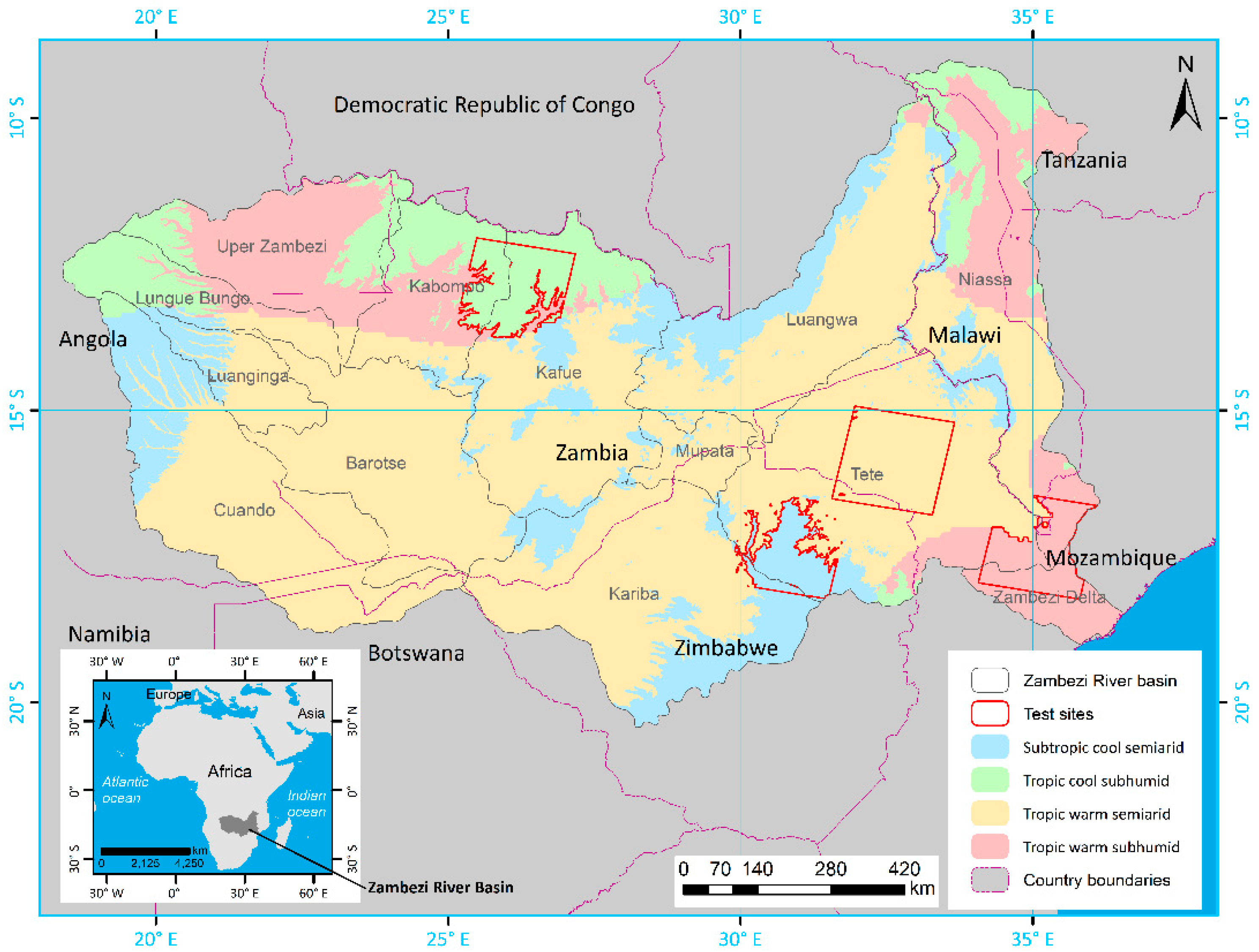
According to [34], the ZRB is composed of four agroecological zones AEZs, namely, tropic cool semiarid, tropic cool sub-humid, tropic warm semiarid, and tropic warm sub-humid zones. Each of these AEZs represents diversified characteristics of cropping practices, field sizes and, heterogeneity of landcover and climate variation [35]. For example, the tropic cool zones are characterized by large field sizes compared to tropic warm zones. These characteristics influence the discrimination of cropland from non-cropland areas. This study aims to investigate the stability of several parametric and non-parametric classifiers for cropland mapping by addressing the diversity in landcover and cropping systems over four different AEZs in the ZRB, taking advantage of multiple fine resolution datasets (Landsat-8 and Sentinel-2), as well as cloud computing with Google Earth Engine (GEE) (https://earthengine.google.com/) [36,37]. The objectives of the paper are (1) to evaluate the feasibility of training samples derived from existing datasets for large-scale cropland mapping and (2) to investigate the stability of four different classifiers (machine learning (random forest, support vector machine, and classification and regression tree) and non-parametric (minimum distance) classifiers) over different AEZs with diverse landscapes and cropping systems.

2. Materials and Methods

2.1. Study Region

The study focused on the Zambezi River basin (ZRB), located in Southern Africa (Figure 1). The Zambezi is the fourth-longest river in Africa [38], and its basin covers an estimated area of approximately 1.38 million km² [39,40]. It stretches from the upper Zambezi in Zambia to the Zambezi delta in Mozambique, with river discharge of approximately 2600 m³ s⁻¹ of water into the Indian Ocean [39,41]. This basin connects eight countries, namely, Angola, Botswana, Malawi, Mozambique, Namibia, Tanzania, Zambia, and Zimbabwe. The largest section of the basin is in Zambia (approximately 40.7% of the total area of the basin), followed by Angola (18.3%). Zimbabwe, Mozambique, Malawi, Botswana, Tanzania, and Namibia represent 15.9%, 11.4%, 7.7%, 2.8%, 2.0% and 1.2% of the total area of the basin, respectively [41].

The ZRB consists of three sections, namely, the Upper Zambezi, which stretches from the headwater to Livingston in Zambia; the Middle Zambezi from Livingston to Cahora Bassa Dam in Tete province in Mozambique; and the Lower Zambezi from the Cahora Bassa Dam to Beira (Zambezi delta) [38,42]. Agriculture is one of the major economic activities of all basin countries. About 70% of the basin population depends on agriculture for subsistence [43]. Over the region, four categories of cropland sizes have been identified, varying from very small field sizes (less than 2.5 ha) to large field sizes (more than 60 ha) [8]. According to [44], the dominant cropping system over the ZRB is rainfed. As a result, agriculture in this region is profoundly affected by rainfall variability [45,46]. Although little rainfall is received during the dry season (April to September), there is a small fraction of the basin that is equipped with irrigation systems to support some agricultural practices performed all year-round.

The climatic conditions in the Zambezi basin follow the seasonal migration of the intertropical convergence zone, hence resulting in distinct hot wet (October to March) and cool dry (April to September) seasons. Specifically, the wet and dry season average precipitation is 137 mm and 14 mm, respectively (Figure 2a), while the temperature averages are 24.2 °C and 20.3 °C, respectively (Figure 2b). A study by [9] indicated that from 1998–2018, the mean annual precipitation recorded in the basin was 965 mm year⁻¹, with the highest precipitation recorded in the northern (more tropical) region. Across the basin, the rainy season coincides with the growing period of most crops. During this period, most of the rainfed crops, such as maize, sorghum, millet, and rice, are planted. Additionally, [9] found that over the period 1998–2017, the peak of precipitation (i.e., 227 mm month⁻¹) occurs in January. In the winter/cool season, the temperature in the basin is low (Figure 2b), making it possible for some farmers to plant wheat and other crops under irrigation since evapotranspiration is low.

In this study, we assessed four different classification methods under various conditions of AEZs within the ZRB. The four AEZs in the basin are, respectively, the tropic cool semiarid, tropic cool sub-humid, tropic warm semiarid, and tropic warm sub-humid zones [34].

2.2. Data and Processing

2.2.1. Remote Sensing Data and Processing

This study used the Landsat-8 and Sentinel-2 image collections covering three consecutive agricultural years (December 2016/November 2017, December 2017/November 2018, and December 2018/November 2019). Six comparable bands (blue, green, red, near infrared (NIR), short wave infrared 1 (SWIR1), and quality band) from Landsat-8 and Sentinel-2 datasets were used. Due to the frequent clouds, which usually occur in the study area, we used the quality bands (Sentinel-2: Quality band at 60 m resolution (Q60) and Landsat-8: Band of Quality Assessment (BQA)) to mask out clouds.

Table 1. Characteristic of the Sentinel-2 and Landsat-8 remote sensing data used in the study.

Sensor	Provider	Bands	Description	Wavelength (nm)	Resolution (m)
Sentinel-2 MultiSpectral Instrument (MSI) Level-1C—Top of Atmosphere (TOA)	European Space Agency (ESA)	B2	Blue	458–523	10
		B3	Green	543–578	10
		B4	Red	650–680	10
		B8	Near-infrared	785–900	10
		B11	SWIR1	1565–1655	20
		QA60	Cloud mask	-	60
Landsat-8 Surface Reflectance Tier 1 TOA	United States Geological Survey (USGS)	B2	Blue	452–512	30
		B3	Green	533–590	30
		B4	Red	636–673	30
		B5	Near-infrared	851–879	30
		B6	SWIR-1	1566–1651	30
		BQA	Quality band	-	-

shows the characteristics of Sentinel-2 and Landsat-8 data used in this study [48].

The processing of the remote sensing data was carried out in the Google Earth Engine (GEE) platform [36]. Five derived remote sensing indices, namely NDVI (normalized difference vegetation index), LSWI (land surface water index), EVI (enhanced vegetation index), BI (bare soil index), SAVI (soil adjusted vegetation index), and GCVI (green chlorophyll vegetation index) were also used as complementary layers for each Landsat-8 and Sentinel-2 images.

Table 2. Remote sensing derived indices used in this study.

Remote Sensing Indices	Formula	Ref.
Normalized Difference Vegetation Index	$NDVI=\frac{NIR-RED}{NIR+RED}$	[52]
Soil Adjusted Vegetation Index	$SAVI=\left(\frac{NIR-RED}{NIR+RED+L}\right)\ast \left(1+L\right)$	[53]
Land Surface Water Index	$LSWI=\frac{NIR-SWIR}{NIR+SWIR}$	[54]
Green Chlorophyll Vegetation Index	$GCVI=\left(\frac{NIR}{GREEN}\right)-1$	[49]
Bare Soil Index	$BI=\left(\frac{\left(RED+SWIR\right)-\left(NIR+BLUE\right)}{\left(RED+SWIR\right)+\left(NIR+BLUE\right)}\right)$	[55]

shows the equations used to calculate these derived indices. Although GVCI is not a commonly used index, it is good at reducing the effect of saturation at high vegetation biomass conditions [49,50]. Researchers applied GCVI in the estimation of leaf area index and green leaf biomass in maize canopies and found that it worked well at both growing and flowering stages [49]. Nearest neighbour bilinear resampling was used to resample the reflectance bands into 10 m, based on which the RS-based indices were derived at a 10 m resolution. To take advantage of all available clear pixels of images and avoid the cloud contamination problems during the rainy season, different integration methods were applied in this study for seasonal composition. The percentile composites at 25%, 50%, 75%, and 95% percentiles were used to compose the derived remote sensing indices (Table 2) during the rainy season while the median composite was used for the dry season. The percentile was used because it can fully capture the spectrum of satellite data and nature vegetation phenological information [51], whereas the median composite reduces the image collection by calculating the median of all values at each pixel across the stack of all matching bands. The yearly stack image used for the subsequent classification process was obtained by combining the two merged images composed for each period (rainy and dry) with a total number of 35 bands as inputs to classifiers (

Table 3. The two seasonal stack images that composed the yearly mosaic.

Rainy Season Stack Image	Dry Season Stack Image
- Five merged bands from Landsat-8 and Sentinel-2 (blue, green, red, NIR, SWIR). - Twenty percentiles (Four percentiles extracted from the merged Landsat-8-derived and Sentinel-2 derived vegetation indices.	- Median composites of five original merged bands from Landsat-8 and Sentinel-2 (blue, green, red, NIR, SWIR 1). - Median composites of five vegetation indices derived from Landsat-8 and Sentinel-2 (NDVI, LSWI, EVI, SAVI, GCVI).

).

2.2.2. Samples

Three available land cover datasets were used to collect the training samples. These datasets included the (i) GFSAD30AFCE at a 30 m spatial resolution, with an overall accuracy of 94.5% [18]; (ii) the ESA-CCI-LC_S2_Prototype land cover map at a 20 m resolution [27] with cropland accuracy of 63%; and (iii) and the ESACCL-LC-L4-300 (ESA Climate Change Initiative—Land Cover project 2017) at 300 m resolution with an overall accuracy of 75.4%. Before generating the training samples, these three datasets were harmonized into generalized land cover datasets with five categories, as listed in

Table 4. Summary of the harmonization process of the different datasets to the five defined land cover classes used in the study.

Final Classes	Original Classes
	GFSAD30AFCE	ESA-CCI-LC_S2_Prototype	ESACCL-LC-L4-300
Cropland	Cropland	Cropland	Cropland, rainfed; Cropland, irrigated or post-flooding; Mosaic cropland (>50%)/natural vegetation (tree, shrub, herbaceous cover) (<50%)
Forest	Non-cropland	Trees cover areas Shrubs cover areas Lichen mosses/sparse vegetation Vegetation aquatic or regularly flooded	Mosaic natural vegetation (tree, shrub, herbaceous cover) (>50%)/cropland (<50%); Tree cover, broadleaved, evergreen, closed to open (>15%); Tree cover, broadleaved, deciduous, closed to open (>15%); Tree cover, needleleaved, evergreen, closed to open (>15%); Tree cover, needleleaved, deciduous, closed to open (>15%); Tree cover, mixed leaf type (broadleaved and needleleaved); Mosaic tree and shrub (>50%)/herbaceous cover (<50%); Mosaic herbaceous cover (>50%)/tree and shrub (<50%); Shrubland; Sparse vegetation (tree, shrub, herbaceous cover) (<15%); Tree cover, flooded, fresh or brakish water; Tree cover, flooded, saline water; Shrub or herbaceous cover, flooded, fresh/saline/brakish water;
Grassland	Non-cropland	Grassland	Grassland
Urban areas	Non-cropland	Built up areas	Urban areas
Water bodies	Water	Open water	Water bodies

. Table 4 shows the lookup table between the original and regrouped classes for each dataset. The GFSAD30AFCE did not have to be modified since it only presents three classes (cropland, non-cropland and water bodies). Both the ESA-CCI-LC_S2_Prototype and the ESACCL-LC-L4-300 were regrouped into five classes, including cropland, forest, grassland, urban areas, and water bodies.

A total of 25,000 random points were generated over different AEZs within the ZRB. The distribution of these sample points considered the five class types as well as the area of each AEZ. For example, the sampling density was higher for an AEZ with a larger area. The values from each land cover dataset were extracted to the random points to examine the agreement among the three datasets. Only the samples with full agreement among all three land cover datasets were kept as training samples. This is based on the hypothesis that samples with full agreement among different datasets are more reliable than partially agreement samples. In total, 7971 training samples (Figure A1) were collected over the ZRB basin, in which 576 samples were from the tropic cool sub-humid zone, 1372 samples from the tropic cool semiarid zone, 1163 samples from the tropic warm sub-humid zone, and 4866 samples from the tropic warm semiarid zone. The sample preparation process was performed using ArcGIS.

The validation samples (Figure A1b) were collected from multiple sources, including (1) visual interpretation of Google Earth high-resolution images and Sentinel-2 images, (2) crowdsourced cropland data from Geo-Wiki (global reference datasets on cropland) [56], and (3) field surveys. The field survey samples were collected by using the GVG (GPS-Video-Geographic Information Systems) mobile app [57] during the three years of 2017–2019. A total of 4639 samples were used as validation samples (Figure A1b), in which 1573 samples were from the field surveys, 869 samples were from Geo-Wiki, and the remaining 2197 samples were from visual interpretation.

2.3. Methods

A comprehensive overview of the methodology used in this study is summarized in Figure 3. A link containing the Google Earth Engine script used in this study is presented in the Supplementary Materials.

2.3.1. Definition of Cropland

We adopted the cropland definition of the Joint Experiment of Crop Assessment and Monitoring (JECAM) network, which defines the annual cropland from a remote sensing perspective as a piece of land of a minimum 0.25 ha (minimum width of 30 m) that is sowed/planted and harvestable at least once within the 12 months after the sowing/planting date. The annual cropland produces an herbaceous cover and is sometimes combined with some tree or woody vegetation [58]. Upon this definition, we considered three consecutive years (2017–2019) in our research, and a site must have been classified as cropland at least once over the three-year period to be considered as cropland.

2.3.2. Four Classifiers

To map the cropland area over the ZRB, four supervised classifiers were selected based on the literature review and performed in GEE [36]. These methods included random forest (RF), the support vector machine (SVM), minimum distance (MD), and the classification and regression tree (CART). The tree-based RF classifier [59] is an ensemble supervised machine learning technique [60] that produces multiple decision trees by using the randomly selected subset of training samples and variables [61]. By considering a collection of tree-structure classifiers [59,60,61], the RF classifier yields reliable classifications [62]. This classifier uses the Gini index (generalization of the binominal variance) [63] to measure inequality [64]. The machine-learning SVM classifier [16] has been applied to optical character recognition [65] as well as to produce improved classification results [66]. This method is a supervised non-parametric statistical learning theory [66,67]. The SVM classifiers minimize the classification error in the unseen dataset [67]. The tree-based framework, i.e., the CART classifier [68], uses historical data and tree-building algorithms to construct the decision tree [22,69]. This classifier consists primarily of three parts: (a) construction of the maximum tree; (b) choice of right tree size; and (c) classification of the new data using a constructed tree [69]. Similar to RF classifiers, the classification and regression trees use the Gini index [70]. By taking advantage of not being only a mathematically simple and computationally efficient technique [71,72], the nonparametric classifier MD [73] has no assumption of datasets regarding the features of interest and does not consider class variability [71,73]. This classifier is based on the MD rule that calculates the spectral distance between the measurement vector for the candidate pixel and the primary vector for each assigned sample [74]. To perform the classification, RF was optimized using the following parameters: number of trees = 100, and minimum size of terminal node = 1. The SVM classifier was optimized with a kernel type of RBF (radial basis function), cost = 10, and gamma = 0.5. Both CART and MD used default parameters.

2.3.3. Assessment Indicators

To test the robustness of different classifiers over different AEZs, one test site in each AEZ (Figure 1) in the ZRB was chosen. Each site corresponds to the intersection of one Landsat tile and AEZ boundary. Over these test sites, we mapped the land cover by using different classification methods and evaluated the accuracy of five different classes (cropland, grassland, forest, urban areas and water bodies). The land cover maps were further reclassified into two classes, namely, cropland and non-cropland. The binary cropland and non-cropland maps were also validated and assessed for accuracy.

The confusion matrix, kappa coefficient, analysis of variance, and Tukey HSD (Honestly Significant Difference) were used to assess the accuracy of the resulting maps as well as to assess the differences between the four classifiers across AEZs. The confusion (error) matrix [75] consisted of a cross-tabulation [13] that compares the mapped class labels with the observed class labels on the ground [13,75,76]. By definition, the kappa coefficient (k) reflects the difference between the actual agreement and the agreement expected by chance [77,78]. As in many statistical tests, the kappa coefficient ranges from −1 to +1. Values situated below zero indicate that there is no agreement between the observed and expected data, a value of zero indicates an agreement that can be obtained by random choices, and a value of 1 represents perfect agreement between the data [77]. As indicated by [77], most of the available documentation about the kappa coefficient cites [79] as the source of the following kappa coefficient (Equation (1)):

$$K=\frac{{{\displaystyle \sum }}_{i=1}^k{x}_{ii}-{{\displaystyle \sum }}_{i=1}^k\left(X_{i+}x{X}_{+i}\right)}{N^2-{{\displaystyle \sum }}_{i=1}^k\left(X_{i+}x{X}_{+i}\right)}$$

(1)

where k = number of rows and columns in error matrix; N = total number of observations; X_ii = observation in row i and column i; X_i+ = marginal total of row i; and X_+i = marginal total of column i.

We assessed the results obtained by the different classifiers by using the analysis of variance (ANOVA) test. ANOVA is a statistical method that uses F-tests [80] to assess differences between several means [80,81]. The study used a two-factor ANOVA without replication [81], i.e., 4 × 4 (four AEZS and four classification methods). In addition to ANOVA, the obtained results were submitted to the Tukey honestly significant difference (HSD) test [82]. The Tukey HSD test is a statistical tool used to determine if the relationship between two sets of data is statistically significant—that is, whether there is a strong chance that an observed numerical change in one value is causally related to an observed change in another value [82]. This test allows the computation of the honestly significant difference between two or more means by using statistical distributions [83]. This test was used to compare the level of differences between the different results. The formula used to compute Tukey’s analysis is shown in Equation (2):

$$HSD=q_{\alpha A}\sqrt{\frac{M{S}_w}{n_k}}$$

(2)

where q_αA represents the relevant critical value of the studentized range statistics, n_k represents the number of scores used in calculating the group means of interest and MS_w represent the mean square width.

Both ANOVA and Tukey’s HSD tests were computed by using the statistic package SISVAR. Based on the validation, the most reliable and stable classifiers were chosen to map the cropland areas over the ZRB.

3. Results

3.1. The Feasibility of Derived Training Samples

In this study, we relied on the full agreement among land cover (LC) datasets to build our training set. To evaluate the feasibility of this approach, we validated the different areas of agreement (full agreement: three datasets agree on the existing or absence of cropland; medium agreement: two out of the three datasets agrees on the existence of cropland; no-agreement: only one dataset confirmed the existence of cropland) using our validation set, as shown in

Table 5. Assessing the accuracy of mapping cropland in the three agreement levels among land cover (LC) datasets.

Agreement	Class	Nc	C	Total	OA %
	C	131	763	894	85.4
Full agreement	Nc	1865	194	2059	90.6
	Total	1996	957	2953	89.0
Median agreement	C	235	748	983	76.1
No-agreement	C	365	338	703	48.1

C: cropland, Nc: non-cropland, and OA: overall accuracy.

. The area of the full agreement was more accurate in distinguishing the cropped from non-cropland areas with an overall accuracy of 89%. This means that the training samples we produced, based on the full agreement, could obtain 11% errors. Nevertheless, this error is less than the tolerance range of sample errors (20%), which could significantly decrease the classification accuracy [84]. Overall, despite the inevitable errors associated with this approach in deriving the training sets, it still a convenient approach to build the training samples for large-scale cropland mapping case studies like the current one, when the field surveys are not an economic or a practical option.

3.2. Performance of Different Classifiers

Figure 4 and

Table A1. Results of overall accuracy (OA) and kappa Coefficient over the different AEZs based on the applied image classification methods.

Overall Accuracy
Agroecological zones	RF	SVM	MD	CART
Tropic Cool Sub-humid	93.8	91.8	84.5	83.5
Tropic Cool Semiarid	87.2	82.9	79.4	82.9
Tropic Warm Sub-humid	85.9	68.5	76.5	68.5
Tropic Warm Semiarid	82.6	69.6	77	72.7
Average of Four AEZs	87.4	78.2	79.4	76.9
Kappa Coefficient
Agroecological zones	RF	SVM	MD	CART
Tropic Cool Sub-humid	0.88	0.83	0.85	0.67
Tropic Cool Semiarid	0.72	0.63	0.53	0.62
Tropic Warm Sub-humid	0.68	0.17	0.42	0.46
Tropic Warm Semiarid	0.6	0.27	0.45	0.33
Average of Four AEZs	0.72	0.48	0.56	0.52

show the overall accuracy (OA) and kappa coefficient (k) for the cropland classification over four AEZs based on the four classification methods. Overall, the results indicated the performance of classification methods varied with AEZs, but RF performed best among the four methods.

The OA from RF in each AEZ was 94%, 87%, 86%, and 83% in the tropic cool sub-humid, tropic cool semiarid regions, tropic warm sub-humid, and tropic warm semiarid regions, respectively. In addition, RF had the highest average OA (87.4%) and averaged k (0.72) among the four classifiers. CART had the lowest average OA (76.9%), while SVM had the lowest average k (0.48) among the four classifiers.

Table 6. Summary of the confusion matrix of land cover maps.

			Random Forest						Support V. Machine						CART						Minimum Distance
			Reference Data
			C	F	G	U	W	UA	C	F	G	U	W	UA	C	F	G	U	W	UA	C	F	G	U	W	UA
Tropical Cool Sub-humid	Classified data	C	45	0	0	0	0	100	42	0	4	0	0	91.3	37	0	1	0	0	97	39	0	2	0	0	95
		F	2	42	6	0	0	84	4	42	8	0	0	77.8	5	42	12	0	0	71	2	42	4	0	0	88
		G	1	0	25	0	0	96	2	0	19	0	0	90.5	6	0	18	0	0	75	7	0	25	0	0	78
		U	0	0	0	7	3	70	0	0	0	6	1	85.7	0	0	0	4	1	80	0	0	0	8	2	80
		W	0	0	1	1	12	86	0	0	1	2	14	82.4	0	0	1	4	14	74	0	0	1	0	13	93
		PA	94	100	78	88	80	* 90.3	88	100	59	75	93	* 84.8	77	100	56	50	93	* 87.6	81	100	78	100	87	* 71.3
Tropical Warm Sub-humid		C	52	3	27	4	2	59	38	14	14	3	0	55	42	5	22	2	1	58	38	0	18	0	0	68
		F	5	47	8	0	0	78	6	30	5	0	0	73	8	40	7	0	0	73	5	46	6	0	0	81
		G	5	1	7	0	0	54	16	7	20	1	1	44	12	6	13	3	1	37	10	5	15	0	2	47
		U	0	0	0	4	0	100	0	0	0	4	1	80	0	0	0	3	0	100	9	0	3	8	1	38
		W	0	0	0	0	21	100	2	0	3	0	21	81	0	0	0	0	21	100	0	0	0	0	20	100
		PA	84	92	17	50	91	* 70.4	61	59	48	50	91	* 60.8	68	78	31	38	91	* 68.3	61	90	36	100	87	* 64
Tropical Warm Semiarid		C	56	2	15	3	1	73	53	14	25	2	0	56	40	5	13	0	1	68	50	1	10	0	1	81
		F	5	46	8	0	0	78	4	44	5	0	0	83	5	42	6	0	0	79	6	46	13	0	0	71
		G	7	11	24	2	0	55	11	1	17	0	1	57	23	12	27	3	0	42	11	12	23	1	0	49
		U	0	0	0	9	0	100	0	0	0	12	0	100	0	0	1	11	0	92	1	0	1	13	0	87
		W	0	0	0	0	30	100	0	0	0	0	30	100	0	0	0	0	30	100	0	0	0	0	30	100
		PA	82	78	51	64	97	* 75.3	78	75	36	86	97	* 71.2	59	71	57	79	97	* 74	74	78	49	93	97	* 68.5
Tropical Cool Semiarid		C	112	2	28	2	0	78	107	11	24	6	0	72	90	2	14	2	0	83	90	0	8	0	0	92
		F	4	90	22	0	0	78	1	80	10	1	0	87	6	86	24	0	0	74	8	82	21	0	0	74
		G	0	0	22	1	0	96	8	5	37	0	0	74	9	5	22	1	0	59	15	15	42	2	0	57
		U	5	0	2	38	0	84	5	1	3	34	0	79	8	4	14	38	0	59	8	0	3	39	0	78
		W	0	0	0	0	16	100	0	0	0	0	16	100	1	0	0	0	16	94	0	0	0	0	16	100
		PA	93	98	30	93	100	* 80.8	88	82	50	83	100	* 78.5	79	89	30	93	100	* 77.1	74	85	57	95	100	* 73.7

* Overall accuracy (%); C—cropland; F—forest; G—grassland; U—urban area; W—water bodies; UA—user accuracy (%); PA—producer accuracy (%).

summarizes the confusion matrix for the land cover maps. According to Table 6, the forest and grassland were the main classes incorrectly mixed with cropland in all AEZs. Another interesting finding is that all classifiers performed better in cool zones (tropic cool sub-humid/semiarid) than the warm zones (tropic warm sub-humid/semiarid). This may due to the higher confusion of the three vegetation classes (cropland, forest, and grassland) in the warm zones (Table 6). Nevertheless, the highest separation between cropland and the other two vegetation classes (forest and grassland) was observed when applying the RF classifier. Meanwhile, when compared to the other classifiers, the MD classifier underestimated the cropland in all four AEZs. This was most visible in the tropic warm sub-humid zone, where cropland area was underestimated by 7%. In the tropic cool sub-humid zone, all classifiers tended to underestimate cropland, with approximately 6%, 3.1%, 20%, and 14% for the RF, SVM, CART, and MD classifiers, respectively. Due to clearly distinct spectral features and temporal patterns of urban and water bodies, these two classes were rarely mixed with cropland. The only exception was found in the tropic cool semiarid zone, where the urban and cropland types were mixed. This zone includes large cities in Zimbabwe (e.g., Harare and Chitungwiza) where urban areas usually have a high proportion of green areas that could be mistakenly classified as a cropland.

The significance level (F-ration>F-critic) obtained in the analysis of variance (ANOVA) test showed that the agroecological zones, as well as the image classification methods, had a significant effect on the obtained results, with a p-value < 0.05.

Table A2. Summary of the analysis of variance computed for the OA.

Source of Variation	SS	df	MS	F	p-Value	F crit
Classification methods	0.0269	3	0.0090	5.6318	0.0188	3.8625
Agroecological zones	0.0507	3	0.0169	10.5938	0.0026	3.8625
Error	0.0143	9	0.0016
Total corrected	0.0919	15
CV (%) =	4.96
Overall mean:	0.8045		The number of observations:			16

SS: Sum of the squares; MS: Mean Square; df: degree of freedom; F: ratio of two variances; p-value: probability value; F critic: Hypothesis acceptance level; CV: Coefficient of Variation.

and

Table A3. Summary of the analysis of variance computed for the k.

Source of Variation	SS	df	MS	F	p-Value	F crit
Classification methods	0.1380	3	0.0460	3.9544	0.0473	3.8625
Agroecological zones	0.4117	3	0.1372	11.7954	0.0018	3.8625
Error	0.1047	9	0.0116
Total corrected	0.6545	15
CV (4%) =	18.98
Overall mean:	0.5683		The number of observations:			16

summarize the analysis of variance computed for both OA and kappa coefficients, respectively. Tukey’s HSD test (

Table 7. Summary of the Tukey honestly significant difference (HSD) test computed for the overall accuracy and kappa coefficient.

Classifier	Overall Accuracy		Kappa Coefficient
	Mean	Test Results	Mean	Test Results
Random Forest	0.8739	a	0.7202	a
Minimum Distance	0.7938	ab	0.5603	ab
Support Vector Machine	0.7816	b	0.5195	ab
Classification and Regression Tree	0.7687	b	0.4734	b
Honestly Significant Difference (HSD)	0.0881		0.2382
Minimal Level of Significance	5% (0.05)

Note: Means followed by the same letter (a, b) do not differ at the 5% minimum level of significance based on Tukey’s HSD test.

) indicated that for the OA, there were no significant differences between the means obtained by the RF and MD classifiers and the means obtained by the SVM and CART classifiers. Concerning the kappa coefficient, significant differences in the means were recorded by the RF and CART classifiers, with corresponding kappa values of 0.72 and 0.47, respectively. In addition, Tukey’s HSD test, calculated using the average OA (0.0881) and kappa coefficient (HSD=0.2382), confirmed the significant differences found by the ANOVA.

3.3. Cropland Extent over the Zambezi River Basin

We mapped the cropland by using the random forest classifier for each AEZ over the ZRB. This classifier was chosen because it showed higher overall accuracy and user accuracy for cropland class than other classifiers (Table 6 and Table A1 and, Figure 4). Figure 5 shows the extracted cropland extent at 10 m over the ZRB, and Figure 6 compares the cropland map from this study with the GFSAD30AFCE. By using independent samples, most from field surveys and high-resolution Google Earth images, we assessed the overall accuracy and kappa coefficient for our binary cropland map. Our overall accuracy was 84%, and the kappa coefficient was 0.67.

Table 8. Confusion matrix for the accuracy assessment of cropland maps in the ZRB.

		Reference Data
	Classes	Non-Cropland	Cropland	Raw Sum	User Accuracy
Classified Data	Non-cropland	2284	312	2596	88.0
	Cropland	439	1604	2043	78.5
	Column sum	2723	1916	4639
	Producer accuracy	83.9	83.7
Overall Accuracy:		84%
Kappa:		0.67

summarizes the confusion matrix for this assessment.

4. Discussion

Suggested by previous studies, field size [8], spatial extent, and landscape patterns [85] are the major factors impacting the accuracy of cropland classification [12]. According to [8], field size can be of great importance in agricultural land monitoring, referring to the fact that, for example, a small field size will require the use of high-resolution images when compared with larger fields. Over the ZRB, the dominant field size is labelled ‘‘very small’’ (0.64–2.56 ha and < 0.64 ha). To handle this issue, different aspects must be taken into consideration, including the methodology to be applied, the characteristics of the land features, and the quality of the input data for classification. The results obtained from this study indicate that with an average OA of 87.4%, the RF classifier outperformed all other classifiers, including MD (79.4%), SVM (78.2%), and CART (76.9%) in all studied AEZs. The good performance of RF classifier over different AEZs indicates it has substantial potential in mapping cropland features under different conditions. Similar findings were reported by [18,21], who used RF to map not only the cropland extent but also the different features on the Earth’s surface. Although RF performed best in all AEZs, this classifier still needs to be trained in each region considering the dynamics of agricultural conditions.

In this study, we found that by training in each region, the accuracies of this classifier varied with the AEZS (Figure 4), with the highest accuracy observed in the tropic cool sub-humid region (93.8%), and the lowest accuracy observed in the tropic warm semiarid region (82.6%). The differences presented here might be attributed to landscape patterns, field sizes, and different cropping systems at different AEZs [86]. For example, the tropic cool zones (semiarid and sub-humid) have different cropping systems and field sizes compared with those of the tropic warm zones (semiarid and sub-humid). In the tropic cool zones, a high percentage of the area is mostly characterized by commercial farms with relatively large field size [8], making it easy to identify the croplands with higher accuracy. In contrast, over the tropic warm (semiarid and sub-humid) zones, the high phenological similarity between vegetation classes, particularly grassland, with rainfed cropland areas could be the main source of confusion. The zone-dependent variations in cropland classification accuracies were also reported by [87] when mapping cropland area over southeast and northeast Asia using multi-year time-series Landsat 30 m data and a random forest classifier. In the process of cropland mapping, one of the biggest challenges is the separation of cropland from grassland. Grassland has, in some growing periods, spectral features similar to those of cropland, which often confuse discrimination from cropland [88]. Some fields have crops in some years while in other years, they are left idle (bare or as grassland), which also leads to spectral variability and confusion in the multi-temporal analysis. This phenomenon may have led to the higher misclassification among cropland, grassland, and forest in the two tropical warm (semiarid and sub-humid) zones than in the two tropical cool (semiarid and sub-humid) zones, leading to the higher accuracy of all four classifiers in cool AEZs (Figure 4).

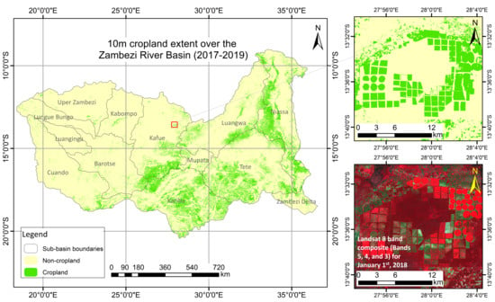
It is noteworthy that our research paid special efforts in collecting and processing the input data to improve the cropland classification thanks to the cloud computing techniques. The cropland extent was finally mapped at a 10 m spatial resolution over the ZRB by considering three years, 2017–2019. We obtained an overall accuracy of 84%, which was 2% higher than the GFSAD30AFCE for the years 2015/2016 over the ZRB [18]. The differences between these two studies are the input datasets. This study enhanced mapping by combining reflective bands with multiple derived indices, thereby increasing spectral discriminability between the different classes. In addition, our 10 m cropland map was also compared to the FROM-GLC 30 m cropland map developed by [84] over the ZRB. It was found that not only did we improve the spatial resolution of cropland map (from 30 m to 10 m), but also the accuracy of our cropland map was 15% higher than that of the FROM-GLC product.

This study also proved the importance of the integration of different types of datasets (Landsat-8 and Sentinel-2) for accurate cropland mapping. In this study, these two different datasets were chosen because most of the study region is characterized by rainfed croplands, and the growing period (an essential element in the identification of cropland areas) coincides with the rainy season, thus, obtaining cloud-free time-series images becomes a challenge. Hence, the use of multiple sensors enhanced the acquisition of cloud-free images, which in turn contributed to more accurate results. Apart from the RF classifier and the usage of the different datasets, another essential element that contributed to the improvement in mapping accuracy was the technique used to collect samples for classifier training/calibration. In this study, the samples used were collected from locations where there was agreement between different existing land cover datasets on the class value at a given point. By using different datasets for sampling, we have reduced the uncertainty and therefore provided more reliable calibration sets. Apart from the RF classifier and the usage of the different datasets, another essential element that contributed to the improvement in mapping accuracy was the technique used to collect samples for classifier training/calibration. In this study, the samples used were collected from locations where there was an agreement between different existing land cover datasets on the class value at a given point. Furthermore, a comparison of spatial agreement of the four different land cover datasets (including GFSAD30AFCE, CGLS-LC100, ESACCILC_S2_Prototype, and ESACCL-LC-L4-300) based on standard deviation [12] revealed high spatial agreement on cropland maps over the ZRB, suggesting that these datasets are reliable over the region. By using different datasets for sampling, we have reduced the uncertainty and therefore provided more reliable calibration sets.

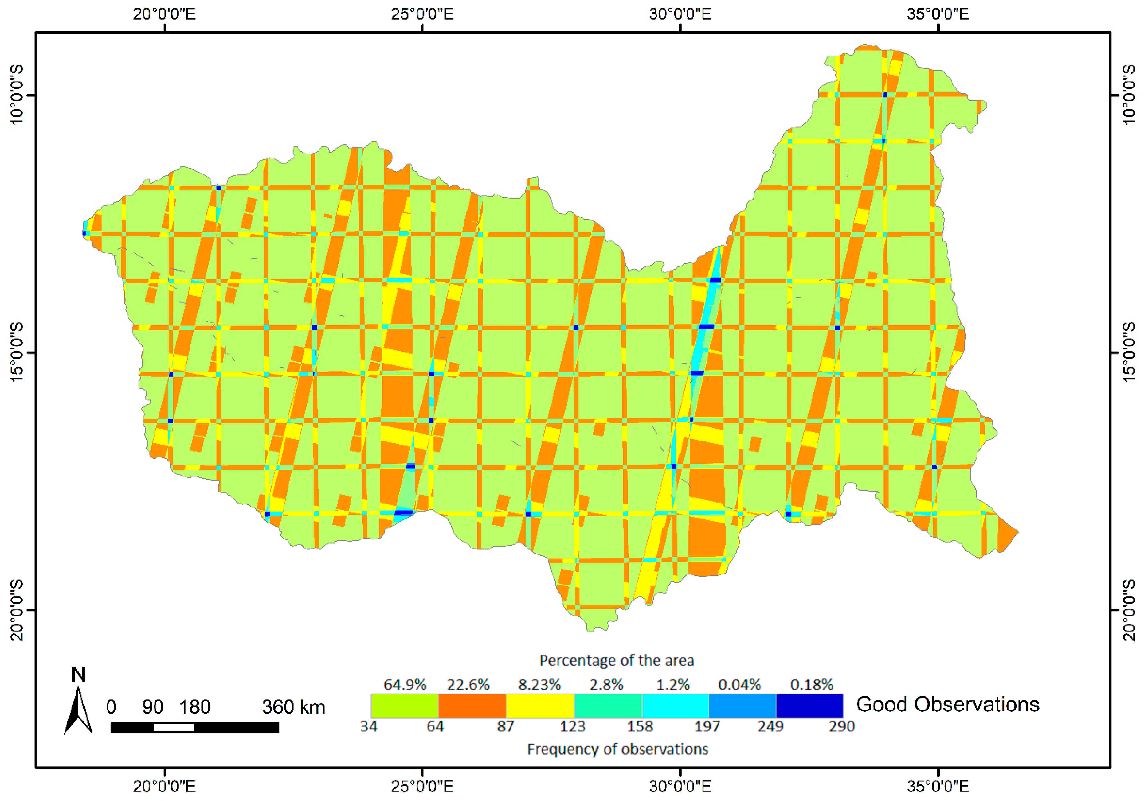
In terms of limitations of this study, the present of cloud is a big issue for RS observations in study area, particularly over the rainy season (October to March). Although a yearly mosaic is used to reduce the impact of clouds, the impact cannot be eliminated. The use of Synthetic Aperture Radar (SAR) data may result in better separation between cropland and grassland, especially in areas close to rives or wetlands which might be another limitation of this research. Fortunately, cloud computing on the GEE platform efficiently processed and composited thousands of imageries for each year. As a consequence, the number of cloudless observations for the rainy season (October 2018 to March 2019) was 64 on average by integrating Landsat-8 and Sentinel-2 imageries (Figure A2). Moreover, 64.9% of the ZRB had 34 to 64 valid observations during the rainy season. Thus, the uncertainty of cloud impacts is limited to some extent. Furthermore, more validation samples based on field surveys are needed for better quality assessment. Given that only a small number of validation samples are available, we relied on a freely available validation dataset, which could also introduce some uncertainty in the final assessment.

5. Conclusions

In this study, we assessed the accuracy of four classifiers for cropland mapping in four different AEZs in the ZRB. Two types of remote sensing data (Landsat-8 and Sentinel-2) and their derived vegetation indices were adopted to improve cropland classification. The results proved the robustness of random forests in obtaining accurate cropland extent through all AEZs. The random forest method outperformed other classifiers and had an average overall accuracy of 87.4% across the four AEZs. Although the other classifiers had lower accuracy than RF, they still performed better than previous research conducted in the basin. The accuracy obtained in this study is higher than various available cropland maps over the ZRB, and this is attributed to the high quality of remote sensing and training data used in this study, as well as the consideration of agriculture diversity, including agro-ecosystems and field sizes (from small farms to commercial farms). The use of high resolution and multi-temporal data improves the discrimination of croplands from other vegetation classes, and also contributes to high accuracy, even in sub-basins with small field sizes. Based on the methodology proposed by this study, cropland maps with a resolution of 10 m could be generated periodically, which would be helpful for the rapid crop monitoring and cropland change analysis in response to the escalating population and food insecurity. The applicability of this method over other areas with similar agroecological conditions (e.g., the Congo River basin in central Africa and the Mekong River basin in southeast Asia) still need to be further investigated.