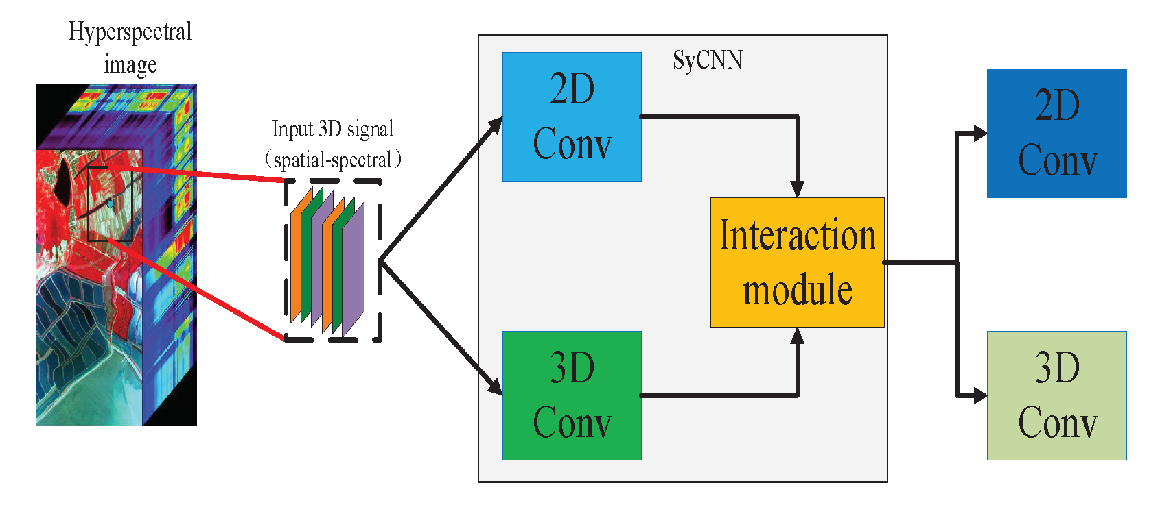
Figure 1.
The Synergistic Convolutional Neural Network (SyCNN) framework which integrates 2D CNN, 3D CNN and the data interaction module for hyper-spectral image classification.
Figure 1.
The Synergistic Convolutional Neural Network (SyCNN) framework which integrates 2D CNN, 3D CNN and the data interaction module for hyper-spectral image classification.
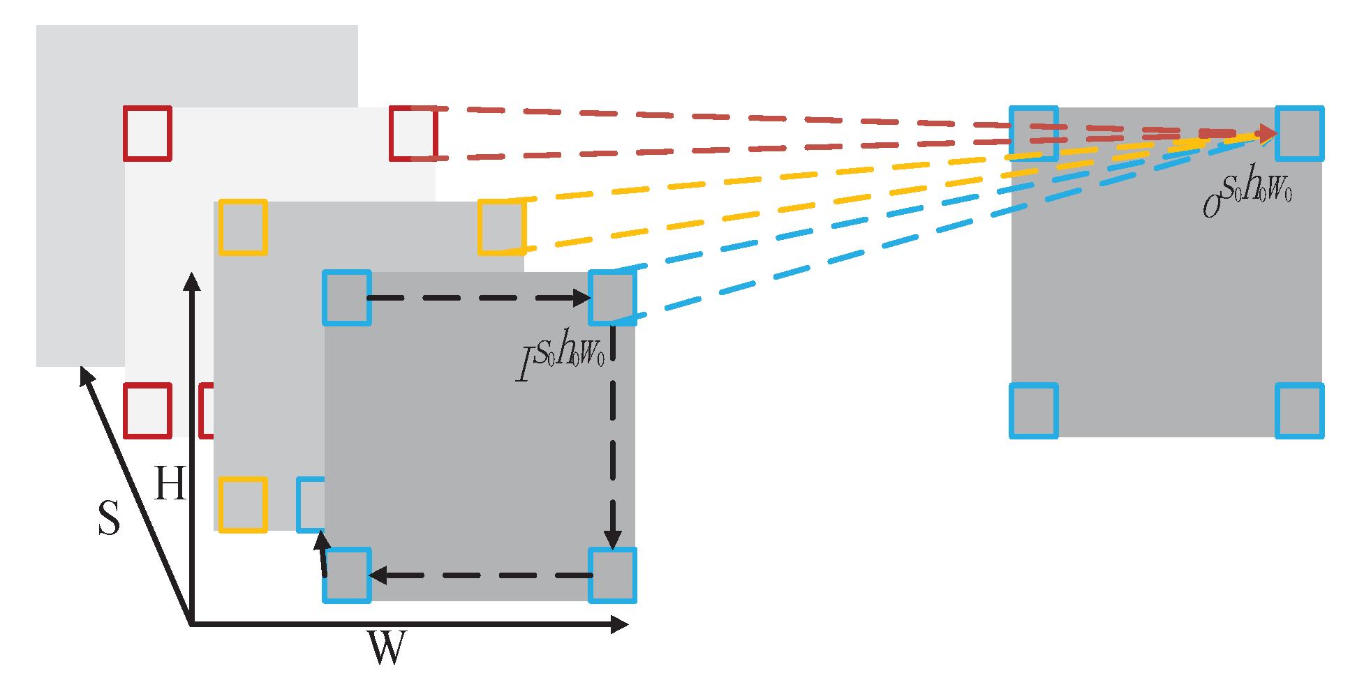
Figure 2.
Illustration of a 3D convolution operation. The convolution kernels slide along both the spatial and spectral dimensions of the input 3D images and generate the 3D spectral–spatial features.
Figure 2.
Illustration of a 3D convolution operation. The convolution kernels slide along both the spatial and spectral dimensions of the input 3D images and generate the 3D spectral–spatial features.
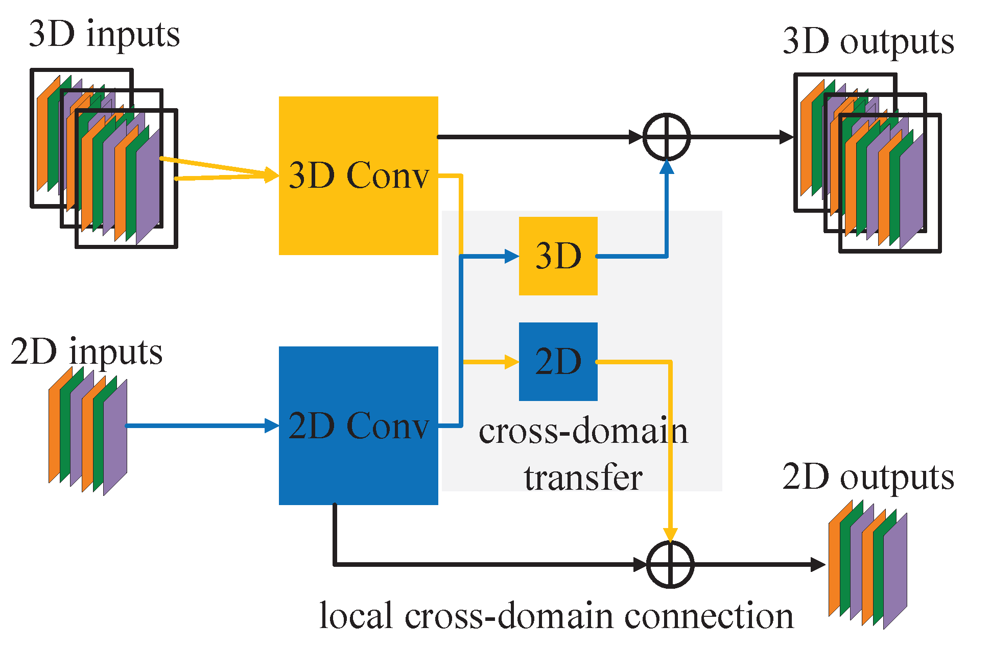
Figure 3.
SyCNN with data interaction module that consists of the local cross-domain connection and cross-domain transfer. 2D spectral–spatial fusion is achieved by transferring the 3D inputs to 2D outputs and concatenating these outputs with the 2D inputs. On the other hand, the 3D spectral–spatial fusion is obtained by transferring the 2D inputs to 3D outputs and concatenating these 3D outputs with the 3D inputs.
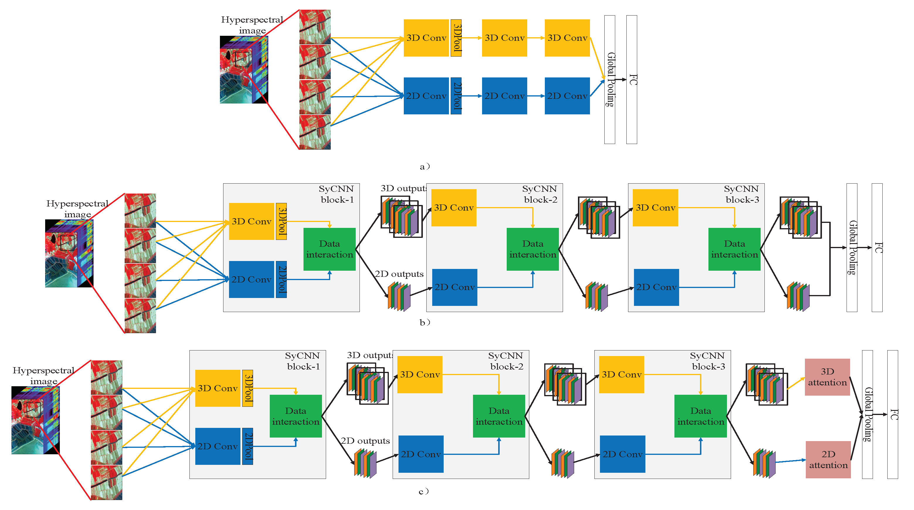
Figure 4.
Illustration of the proposed models: (a) The deep simple SyCNN model, (b) the deep SyCNN model, (c) the deep SyCNN with attention module. Yellow blocks and blue blocks refer to 3D convolution and 2D convolution. Green blocks refer to data interaction module.
Figure 4.
Illustration of the proposed models: (a) The deep simple SyCNN model, (b) the deep SyCNN model, (c) the deep SyCNN with attention module. Yellow blocks and blue blocks refer to 3D convolution and 2D convolution. Green blocks refer to data interaction module.
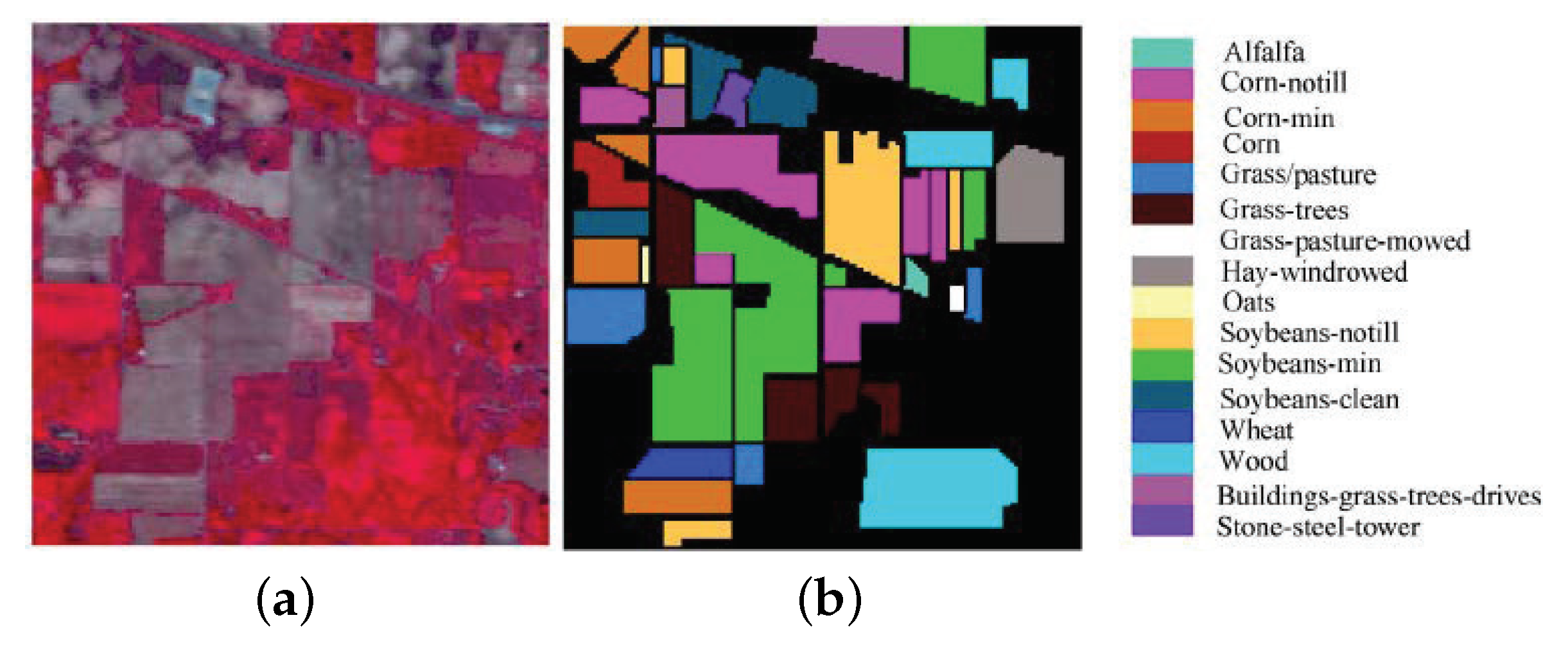
Figure 5.
Indian Pines dataset. (a) Three-band false-color composite. (b) Ground-truth map.
Figure 5.
Indian Pines dataset. (a) Three-band false-color composite. (b) Ground-truth map.
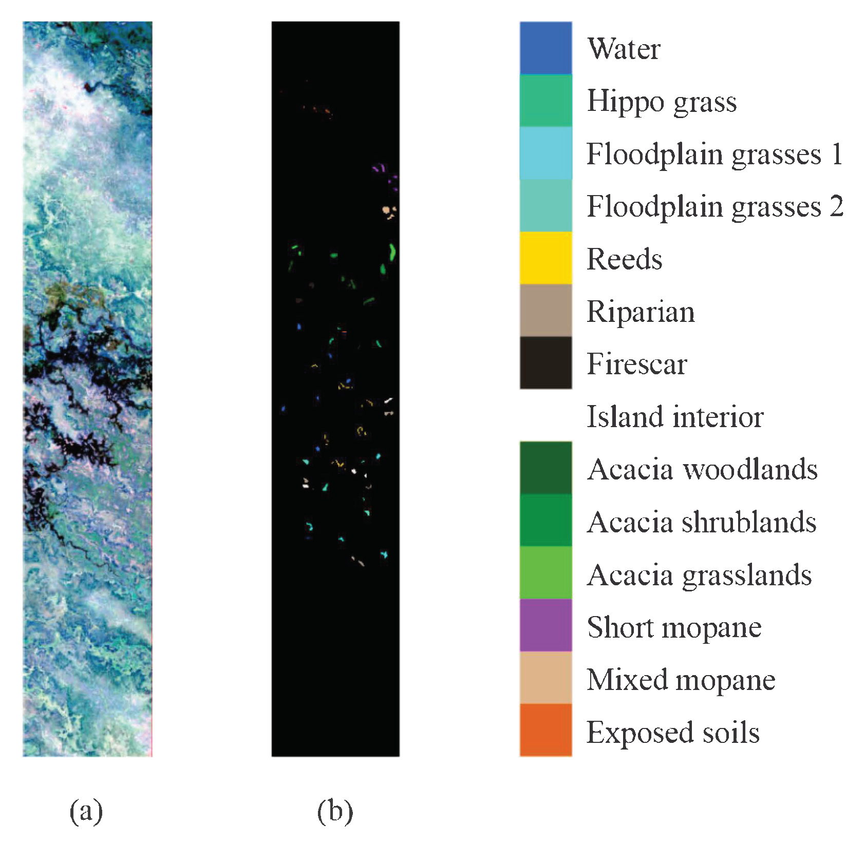
Figure 6.
Botswana Scene dataset. (a) Three-band false-color composite. (b) Ground-truth map.
Figure 6.
Botswana Scene dataset. (a) Three-band false-color composite. (b) Ground-truth map.
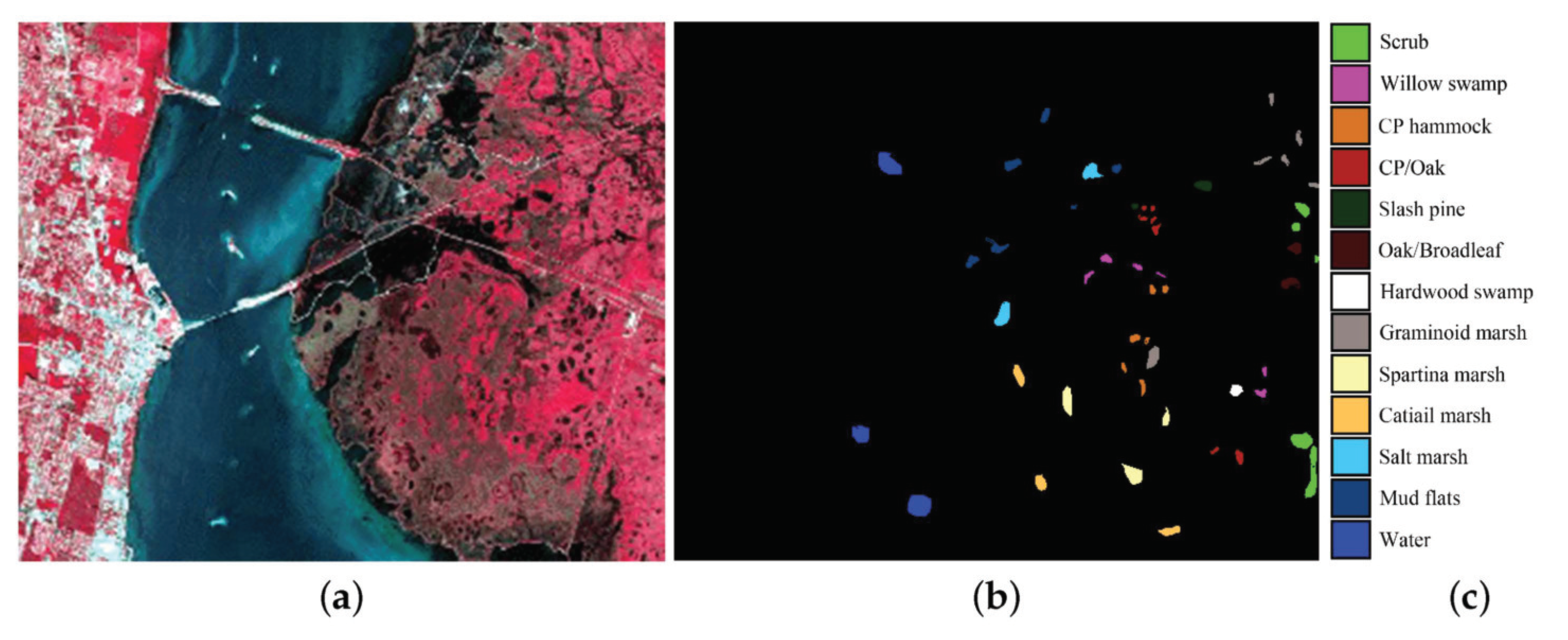
Figure 7.
Kennedy Space Center dataset. (a) Three-band false-color composite. (b) Ground-truth map.
Figure 7.
Kennedy Space Center dataset. (a) Three-band false-color composite. (b) Ground-truth map.
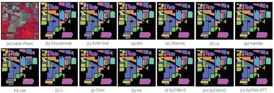
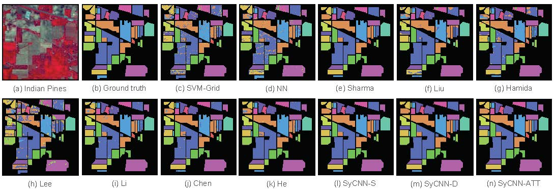
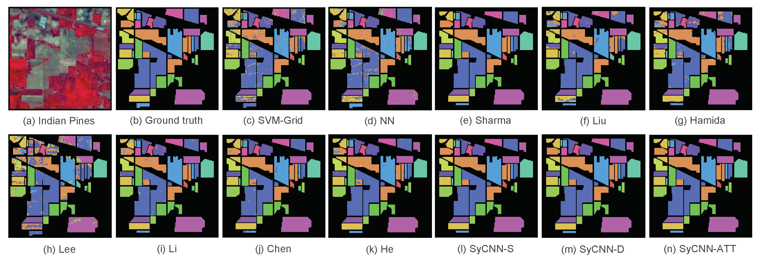
Figure 8.
Visualization of the experimental results based on Indian Pines: (a) Indian Pines, (b) Ground truth, (c) SVM-Grid, (d) NN, (e) Sharma, (f) Liu, (g) Hamida, (h) Lee, (i) Li, (j) Chen, (k) He, (l) SyCNN-S, (m) SyCNN-D, (n) SyCNN-ATT. It is observed that the outputs produced by our proposed models are quite close to the Ground truth.
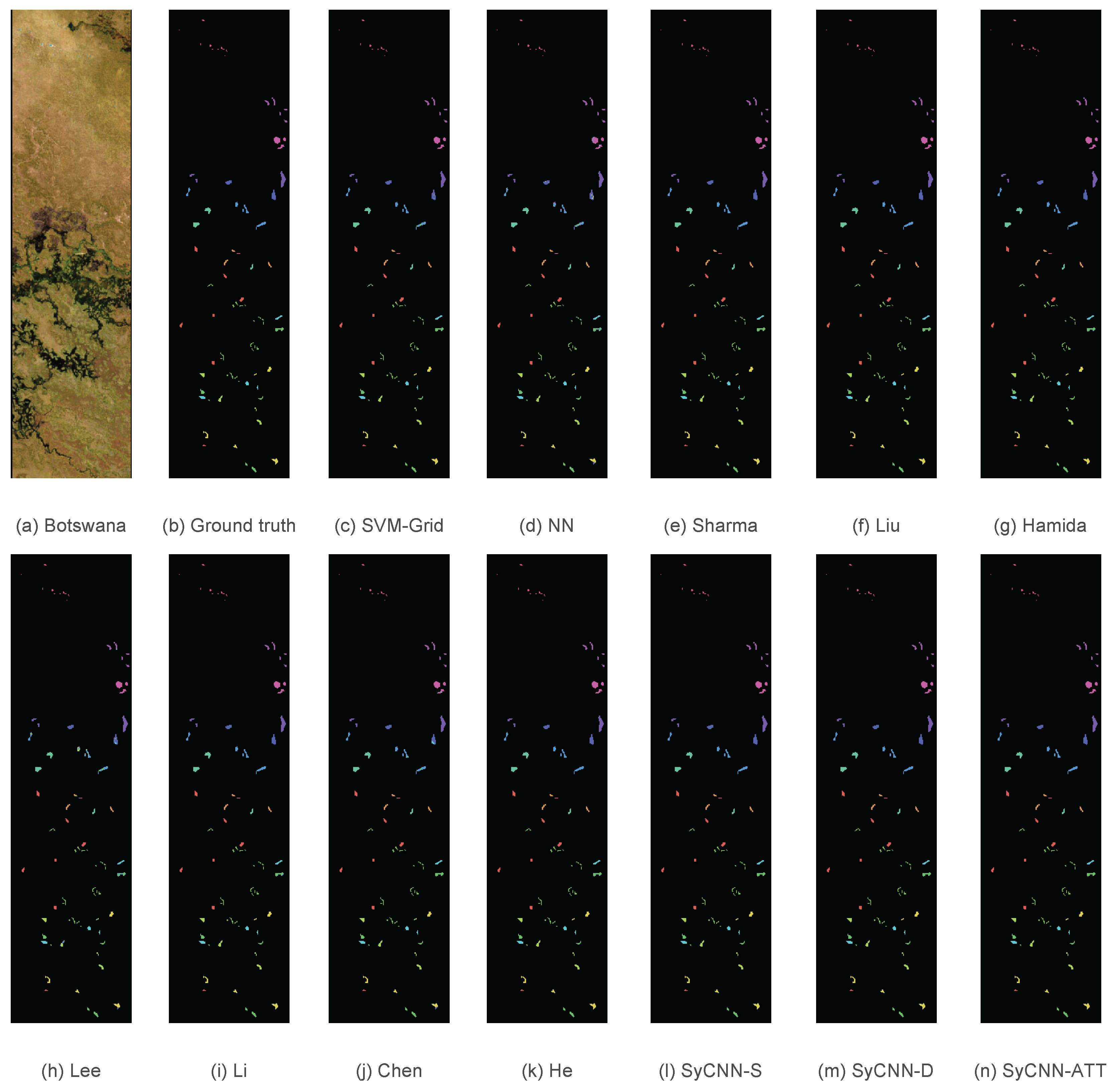
Figure 9.
Visualization of the experimental results based on Botswana: (a) Indian Pines, (b) Ground truth, (c) SVM-Grid, (d) NN, (e) Sharma, (f) Liu, (g) Hamida, (h) Lee, (i) Li, (j) Chen, (k) He, (l) SyCNN-S, (m) SyCNN-D, (n) SyCNN-ATT. It is observed that the outputs produced by our proposed models are quite close to the Ground truth.
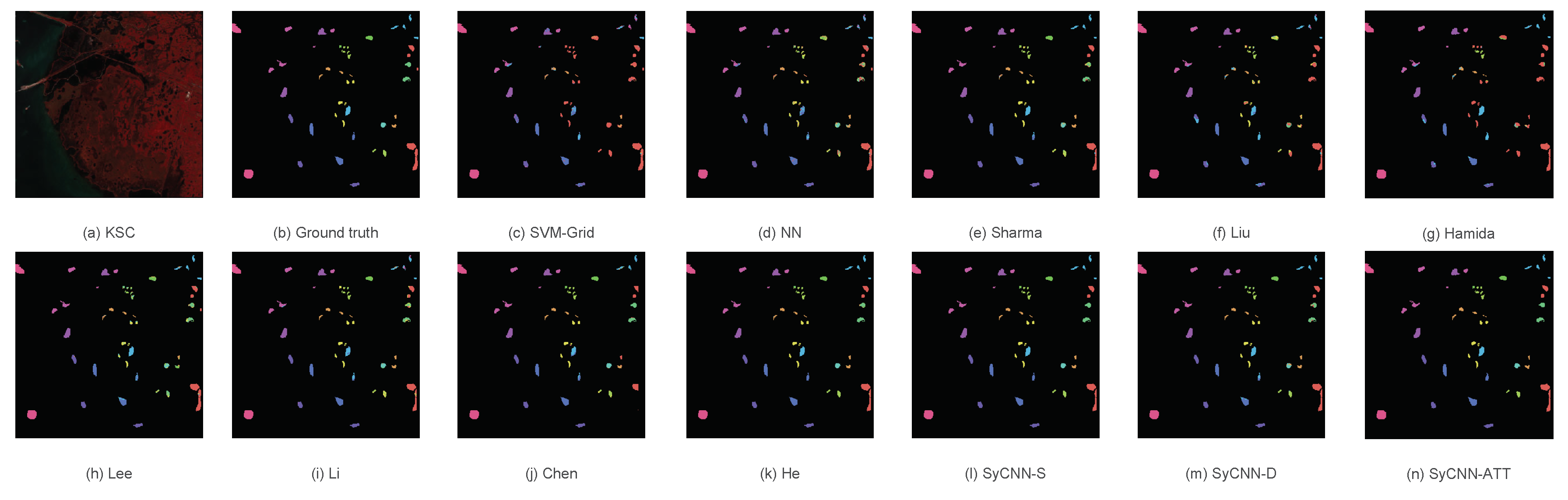
Figure 10.
Visualization of the experimental results based on KSC: (a) Indian Pines, (b) Ground truth, (c) SVM-Grid, (d) NN, (e) Sharma, (f) Liu, (g) Hamida, (h) Lee, (i) Li, (j) Chen, (k) He, (l) SyCNN-S, (m) SyCNN-D, (n) SyCNN-ATT. It is observed that the outputs produced by our proposed models are quite close to the Ground truth.
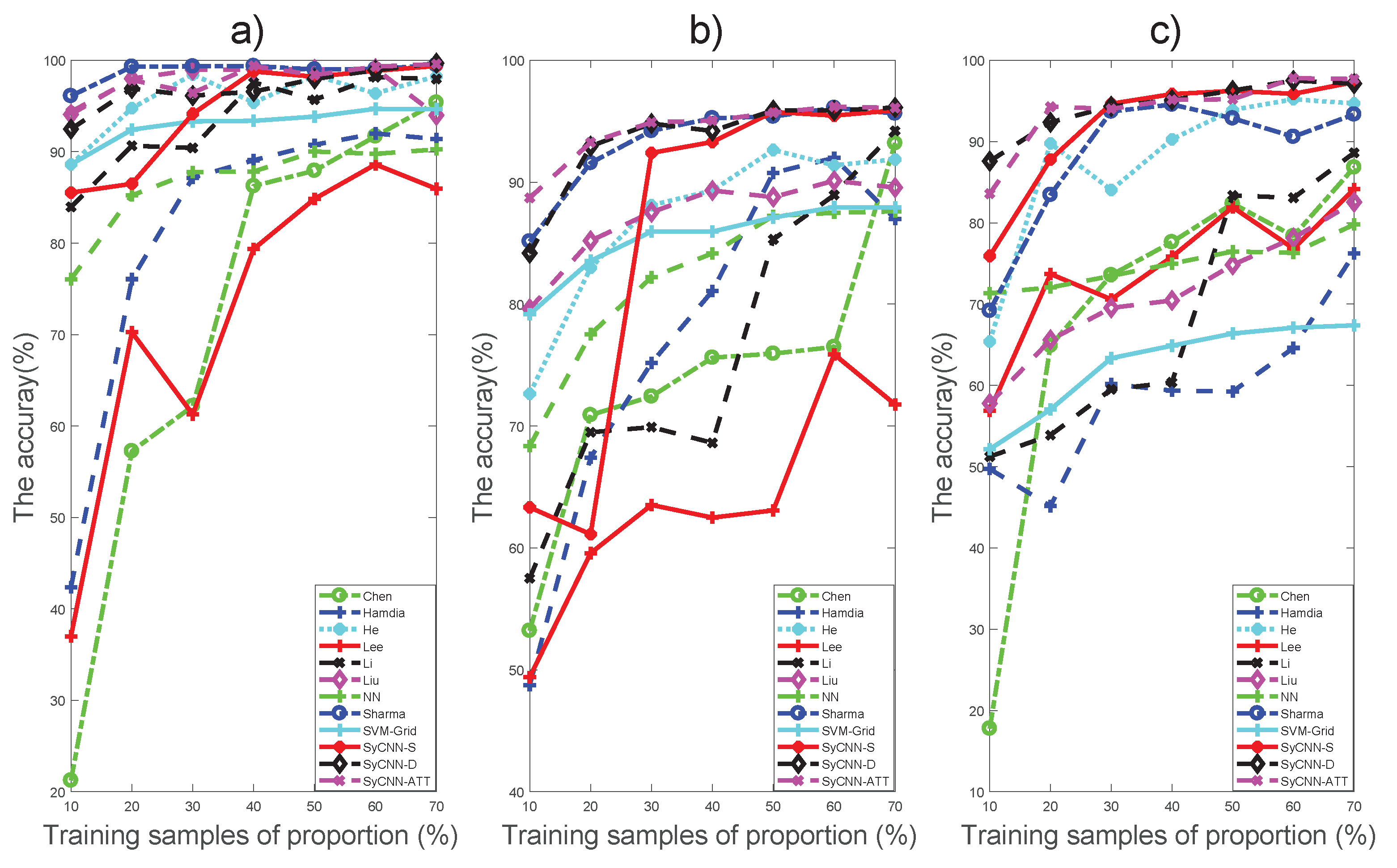
Figure 11.
Visualization of the influence of training samples proportion for different methods based on the three datasets: (a) Indian Pines, (b) Botswana, (c) KSC. It can be observed that the results of our proposed models are very stable and better than the comparison methods.
Figure 11.
Visualization of the influence of training samples proportion for different methods based on the three datasets: (a) Indian Pines, (b) Botswana, (c) KSC. It can be observed that the results of our proposed models are very stable and better than the comparison methods.
Table 1.
Sample size for Indian Pines Scene.
Table 1.
Sample size for Indian Pines Scene.
| NO. | Class Name | Training Samples | Testing Samples |
|---|
| 1 | Alfalfa | 32 | 14 |
| 2 | Corn-notill | 1003 | 424 |
| 3 | Corn-mintill | 585 | 245 |
| 4 | Corn | 168 | 69 |
| 5 | Grass-pasture | 340 | 143 |
| 6 | Grass-trees | 512 | 216 |
| 7 | Grass-pasture-mowed | 20 | 8 |
| 8 | Hay-windrowed | 335 | 143 |
| 9 | Oats | 14 | 6 |
| 10 | Soybean-notill | 683 | 289 |
| 11 | Soybean-mintill | 1721 | 733 |
| 12 | Soybean-clean | 417 | 174 |
| 13 | Wheat | 144 | 61 |
| 14 | Woods | 888 | 374 |
| 15 | Buildings-Grass-Trees-Drives | 272 | 113 |
| 16 | Stone-Steel-Towers | 65 | 28 |
| Total | 7200 | 3040 |
Table 2.
Sample size for Botswana Scene.
Table 2.
Sample size for Botswana Scene.
| NO. | Class Name | Training Samples | Testing Samples |
|---|
| 1 | Water | 189 | 81 |
| 2 | Hippo grass | 71 | 30 |
| 3 | Floodplain grasses 1 | 176 | 75 |
| 4 | Floodplain grasses 2 | 151 | 64 |
| 5 | Reeds | 188 | 81 |
| 6 | Riparian | 188 | 81 |
| 7 | Fire scar | 183 | 76 |
| 8 | Island interior | 143 | 60 |
| 9 | Acacia woodlands | 220 | 94 |
| 10 | Acacia shrunblands | 174 | 74 |
| 11 | Acacia grasslands | 214 | 91 |
| 12 | Short mopane | 127 | 54 |
| 13 | Mixed mopane | 189 | 79 |
| 14 | Exposed soils | 67 | 28 |
| Total | 2280 | 968 |
Table 3.
Samples size for Kennedy Space Center scene.
Table 3.
Samples size for Kennedy Space Center scene.
| NO. | Class Name | Training Samples | Testing Samples |
|---|
| 1 | Scrub | 533 | 228 |
| 2 | Willow swamp | 170 | 73 |
| 3 | Cabbage palm hammock | 179 | 77 |
| 4 | Cabbage palm/oak hammock | 176 | 76 |
| 5 | Slash pine | 113 | 48 |
| 6 | Oak/broadleaf hammock | 160 | 69 |
| 7 | Hardwood swamp | 74 | 31 |
| 8 | Graminoid marsh | 302 | 129 |
| 9 | Spartina marsh | 364 | 156 |
| 10 | Cattail marsh | 284 | 120 |
| 11 | Salt marsh | 294 | 125 |
| 12 | Mud flats | 352 | 151 |
| 13 | Water | 649 | 278 |
| Total | 3650 | 1561 |
Table 4.
Evaluation results on the Indian Pines Scene dataset.
Table 4.
Evaluation results on the Indian Pines Scene dataset.
| Class | Methods |
|---|
| # | SVM-Grid | NN | Sharma | Liu | Hamida | Lee | Li | Chen | He | SyCNN-S | SyCNN-D | SyCNN-ATT |
| 1 | 88.00 | 92.30 | 100 | 66.70 | 100 | 63.60 | 100 | 96.30 | 100 | 100 | 100 | 100 |
| 2 | 85.50 | 84.20 | 99.40 | 88.50 | 84.90 | 82.40 | 96.60 | 95.90 | 89.00 | 100 | 99.60 | 99.20 |
| 3 | 80.80 | 80.30 | 93.60 | 86.10 | 79.70 | 80.40 | 90.60 | 91.10 | 86.00 | 91.30 | 91.70 | 96.10 |
| 4 | 79.20 | 71.90 | 100 | 83.60 | 93.60 | 82.80 | 95.80 | 97.20 | 95.00 | 97.10 | 100 | 99.30 |
| 5 | 95.20 | 93.70 | 94.60 | 91.60 | 93.80 | 93.70 | 94.50 | 92.60 | 95.70 | 96.10 | 95.30 | 97.20 |
| 6 | 96.70 | 96.10 | 100 | 98.40 | 99.10 | 97.50 | 99.80 | 99.10 | 100 | 100 | 99.50 | 100 |
| 7 | 80.00 | 93.30 | 100 | 40.00 | 76.90 | 82.40 | 100 | 93.30 | 100 | 100 | 100 | 100 |
| 8 | 99.00 | 99.30 | 100 | 96.30 | 99.00 | 97.30 | 99.70 | 99.70 | 100 | 100 | 100 | 100 |
| 9 | 66.70 | 100 | 100 | 0 | 90.90 | 28.30 | 100 | 100 | 50.00 | 100 | 100 | 100 |
| 10 | 80.60 | 82.40 | 97.00 | 89.30 | 76.20 | 84.20 | 96.10 | 90.50 | 91.90 | 97.70 | 97.00 | 98.30 |
| 11 | 84.90 | 87.90 | 97.50 | 91.50 | 87.40 | 89.80 | 96.20 | 94.70 | 92.60 | 98.10 | 98.00 | 98.70 |
| 12 | 89.30 | 83.10 | 97.20 | 89.70 | 87.70 | 79.70 | 96.20 | 96.90 | 93.80 | 98.30 | 98.90 | 98.60 |
| 13 | 100 | 100 | 100 | 100 | 100 | 96.10 | 100 | 100 | 100 | 100 | 100 | 100 |
| 14 | 95.80 | 93.50 | 99.70 | 98.40 | 98.90 | 94.20 | 99.70 | 98.90 | 99.10 | 100 | 100 | 100 |
| 15 | 76.70 | 69.10 | 84.20 | 77.20 | 76.30 | 72.00 | 82.20 | 83.70 | 85.80 | 86.80 | 91.10 | 87.40 |
| 16 | 100 | 98.20 | 96.40 | 100 | 98.20 | 100 | 100 | 98.20 | 96.40 | 100 | 98.20 | 100 |
| OA | 87.93 | 87.57 | 95.64 | 89.56 | 86.99 | 87.87 | 94.22 | 93.20 | 91.87 | 95.90 | 96.13 | 97.31 |
| F1 | 87.40 | 89.07 | 97.48 | 81.08 | 90.16 | 83.42 | 96.71 | 95.51 | 92.21 | 97.84 | 98.08 | 98.43 |
| K | 86.20 | 85.80 | 95.10 | 88.10 | 85.20 | 86.10 | 93.40 | 92.30 | 90.80 | 95.30 | 95.60 | 96.90 |
Table 5.
Comparative evaluation based on the Botswana Scene dataset.
Table 5.
Comparative evaluation based on the Botswana Scene dataset.
| Class | Methods |
|---|
| # | SVM-Grid | NN | Sharma | Liu | Hamida | Lee | Li | Chen | He | SyCNN-S | SyCNN-D | SyCNN-ATT |
| 1 | 99.40 | 100 | 99.40 | 100 | 100 | 100 | 100 | 100 | 100 | 100 | 100 | 100 |
| 2 | 98.40 | 96.80 | 100 | 96.60 | 92.90 | 98.40 | 100 | 100 | 100 | 98.40 | 100 | 100 |
| 3 | 98.60 | 92.90 | 100 | 100 | 96.60 | 91.70 | 100 | 100 | 100 | 100 | 100 | 100 |
| 4 | 97.70 | 90.30 | 100 | 100 | 92.70 | 69.30 | 99.20 | 91.40 | 97.70 | 100 | 100 | 100 |
| 5 | 92.40 | 81.50 | 98.80 | 95.20 | 91.00 | 83.70 | 94.90 | 97.70 | 93.40 | 98.80 | 100 | 100 |
| 6 | 87.40 | 74.40 | 99.40 | 92.10 | 72.60 | 76.10 | 91.00 | 92.90 | 91.30 | 100 | 100 | 100 |
| 7 | 98.70 | 99.40 | 100 | 100 | 100 | 99.40 | 100 | 89.30 | 100 | 100 | 100 | 100 |
| 8 | 100 | 97.50 | 100 | 100 | 97.60 | 76.90 | 100 | 98.10 | 100 | 100 | 100 | 100 |
| 9 | 90.20 | 85.10 | 100 | 96.10 | 64.70 | 61.70 | 100 | 93.80 | 97.40 | 100 | 100 | 100 |
| 10 | 90.30 | 83.90 | 99.30 | 97.90 | 97.40 | 81.70 | 100 | 94.40 | 100 | 100 | 100 | 100 |
| 11 | 94.40 | 93.10 | 99.50 | 97.90 | 95.50 | 95.60 | 100 | 91.50 | 100 | 100 | 100 | 100 |
| 12 | 91.40 | 95.40 | 98.10 | 99.10 | 97.10 | 90.60 | 96.20 | 96.20 | 99.10 | 95.20 | 97.10 | 99.10 |
| 13 | 93.90 | 87.70 | 100 | 100 | 99.40 | 100 | 100 | 99.40 | 100 | 100 | 100 | 100 |
| 14 | 100 | 96.70 | 100 | 100 | 90.60 | 88.50 | 100 | 92.60 | 100 | 100 | 100 | 100 |
| OA | 94.66 | 90.25 | 99.48 | 97.49 | 91.38 | 85.94 | 97.94 | 95.38 | 98.25 | 99.38 | 99.69 | 99.79 |
| F1 | 95.20 | 91.05 | 99.61 | 99.68 | 92.01 | 86.34 | 98.36 | 95.52 | 98.49 | 99.46 | 99.79 | 99.93 |
| K | 94.20 | 89.40 | 99.40 | 97.80 | 90.70 | 84.80 | 97.80 | 95.00 | 98.10 | 99.30 | 99.70 | 99.80 |
Table 6.
Classification results of the Salinas scene.
Table 6.
Classification results of the Salinas scene.
| Class | Methods |
|---|
| # | SVM-Grid | NN | Sharma | Liu | Hamida | Lee | Li | Chen | He | SyCNN-S | SyCNN-D | SyCNN-ATT |
| 1 | 57.80 | 87.60 | 89.40 | 81.50 | 69.40 | 94.50 | 87.40 | 54.10 | 91.40 | 94.40 | 94.70 | 97.80 |
| 2 | 72.50 | 71.30 | 94.50 | 80.00 | 61.80 | 68.80 | 91.20 | 88.60 | 93.40 | 98.60 | 99.30 | 99.30 |
| 3 | 0 | 62.40 | 92.20 | 68.30 | 7.50 | 72.20 | 69.20 | 91.40 | 95.10 | 96.70 | 100 | 100 |
| 4 | 0 | 24.10 | 76.60 | 60.90 | 40.70 | 7.30 | 70.30 | 91.50 | 75.20 | 94.60 | 98.70 | 100 |
| 5 | 0 | 53.70 | 88.90 | 61.70 | 31.60 | 67.40 | 82.20 | 100 | 86.30 | 95.90 | 97.90 | 96.80 |
| 6 | 0 | 30.80 | 67.30 | 42.20 | 2.90 | 64.20 | 76.30 | 98.50 | 87.80 | 98.60 | 99.30 | 100 |
| 7 | 0 | 54.20 | 92.50 | 85.30 | 5.60 | 35.00 | 90.00 | 96.80 | 98.40 | 98.50 | 100 | 100 |
| 8 | 41.60 | 61.40 | 94.30 | 72.70 | 70.20 | 80.00 | 81.40 | 82.80 | 97.20 | 98.00 | 96.40 | 97.70 |
| 9 | 73.40 | 83.10 | 99.40 | 84.50 | 85.30 | 95.70 | 91.10 | 93.30 | 99.40 | 100 | 100 | 100 |
| 10 | 83.50 | 88.10 | 99.60 | 96.60 | 77.10 | 86.30 | 96.70 | 100 | 99.20 | 100 | 100 | 100 |
| 11 | 96.00 | 98.40 | 100 | 100 | 99.60 | 98.80 | 99.60 | 100 | 100 | 100 | 100 | 100 |
| 12 | 74.80 | 85.30 | 99.70 | 95.00 | 87.10 | 85.00 | 93.50 | 100 | 99.00 | 99.70 | 100 | 100 |
| 13 | 96.70 | 99.50 | 100 | 99.60 | 99.80 | 97.30 | 100 | 100 | 100 | 100 | 100 | 100 |
| OA | 67.39 | 79.79 | 93.35 | 84.27 | 76.22 | 84.14 | 88.62 | 86.83 | 94.69 | 97.44 | 97.76 | 98.92 |
| F1 | 45.89 | 67.37 | 91.88 | 79.10 | 62.82 | 73.27 | 86.84 | 92.08 | 94.03 | 98.46 | 98.95 | 99.35 |
| K | 62.80 | 77.40 | 92.60 | 82.50 | 73.10 | 82.30 | 87.40 | 85.50 | 94.10 | 97.20 | 97.50 | 98.80 |
Table 7.
Comparison of parameters and times of all methods.
Table 7.
Comparison of parameters and times of all methods.
| Methods | Number of Parameters | Execution Time (s) | OA |
|---|
| SVM-Grid | 2.98 MB | - | 67.39 |
| NN | 65.52 MB | 20.57 | 79.79 |
| Sharma | 5.9 KB | 25.86 | 93.35 |
| Liu | 4.08 MB | 8282.78 | 84.27 |
| Hamida | 472 KB | 46.88 | 76.22 |
| Lee | 1.22 MB | 128.29 | 84.14 |
| Li | 2.38 MB | 37.90 | 88.62 |
| Chen | 3.27 MB | 285.63 | 86.83 |
| He | 8.18 KB | 98.67 | 94.69 |
| SyCNN-S | 21.14 MB | 117.03 | 97.44 |
| SyCNN-D | 29.46 MB | 146.52 | 97.76 |
| SyCNN-ATT | 34.98 MB | 154.15 | 98.92 |

 ,
, 


