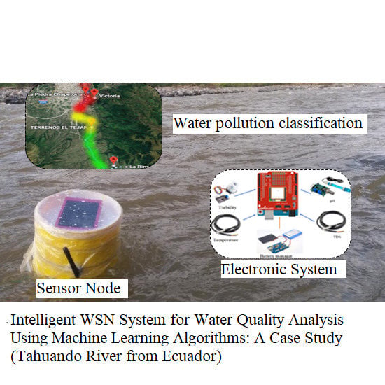
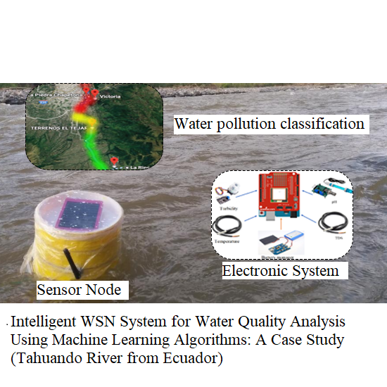
Intelligent WSN System for Water Quality Analysis Using Machine Learning Algorithms: A Case Study (Tahuando River from Ecuador)

Abstract

This work presents a wireless sensor network (WSN) system able to determine the water quality of rivers. Particularly, we consider the Tahuando River from Ibarra, Ecuador, as a case study. The main goal of this research is to determine the river’s status throughout its route, by generating data reports into an interactive user interface. To this end, we use an array of sensors collecting several measures such as: turbidity, temperature, water quality, pH, and temperature. Subsequently, from the information collected on an Internet-of-Things (IoT) server, we develop a data analysis scheme with both data representation and supervised classification. As an important result, our system outputs a map that shows the contamination levels of the river at different regions. Furthermore, in terms of data analysis performance, the proposed system reduces the data matrix by 97% from its original size, while it reaches a classification performance over 90%. Furthermore, as an additional remarkable result, we here introduce the so-called quantitative metric of balance (QMB), which measures the balance or ratio between performance and power consumption.

1. Introduction

Rivers are natural watercourses that commonly come from both precipitation (surface runoff), and snowpacks (e.g., water stored in glaciers). Regularly, they flow towards lakes, sea, oceans, or another river. Urban rivers are responsible for providing water resources to crops and human beings as well as navigation purposes. Certainly, this natural resource may not be everlasting. As a matter of fact, there is currently a great deficit of water reserves due to deforestation, inappropriate and excessive use of fertilizers and pesticides, causing environmental issues [1,2]. Likewise, the urbanization and industries have had collateral adverse impact directly on the water quality of river ecosystems worldwide [3]. Besides, the population growth produces enormous wastewater that enters into the rivers without any environmental control. United Nations (UN) settled that 90% of such waste is not correctly treated, and 70% of the industries discharge contaminant content without any adequate standards or rigorous inspections [4,5]. Water pollution contains high levels of biochemical oxygen demand (BOD), nitrogen, and phosphorus. So it is necessary to develop systems that support the detection and measuring of the contamination levels in rivers to maintain an optimal ecological balance, limiting environmental damage and preventing diseases spread [6]. Consequently, city governments have stated environmental policies intended to create urban regeneration initiatives around the care of their rivers [7]. In this connection, Ecuador, as our case study, has no any short or long-term plan to improve either the urban or rural river conditions [8].

Traditionally, water quality monitoring uses collected samples for laboratory testing, enabling then a wide range of analyses. Notwithstanding, it results impractical to manually measure water pollution at different points along the river. Moreover, this sort of tests may take a few days, and probably not reaching as a good precision as that of in-situ sampling [9]. Nowadays, the use of sensors for monitoring environmental conditions has received significant attention due to the real-time data collection, flexibility, and portability [4,10]. Following from this, the creation of a wireless sensor network (WSN) that combines several sensors with a data processing system and wireless communication can allow for an adequate measure of the water quality, where each sensor becomes a node that shares information among them as well as to a central server [11,12]. Thus, these data are greatly useful for further robust analyzes of water pollution in rivers. However, the large amount of data demands the implementation of machine learning algorithms to create systems that automatically can detect high levels of water pollution and make proper decisions. For that purpose, historical data (training data) become valuable to turn WSN nodes into intelligent systems [13,14].

Consequently, this work presents a novel system composed of three WSN nodes for monitoring in real-time the water pollution present in the Tahuando River (located in Ibarra, Ecuador) using machine learning algorithms. To do so, we establish different measurement points wherein each WSN node acquires the river’s conditions data to be later processed internally by the system. In this sense, we consider water-quality variables, namely pH, turbidity, temperature and dissolved solids. Additionally, we carry out a sensor integration and calibration stage for eliminating reading errors. Finally, we sent these data to a cloud server, using a mobile network, where we visualize the node’s information with its proper geo-location. As relevant results, a reduction of the required training set of 97% is accomplished by using is the condensed nearest neighbor (CNN) method as a prototype selection approach, as well as the classification stage—with k-NN—reaches 90.6% of performance. Then, our work is an exploratory study on different methods for both prototype selection and data classification applied to water treatment. Therefore, we have no gold standard result or benchmark method. Instead, an exhaustive comparison of representative methods is presented.

The fact that the data analysis process is implemented directly into the WSN represents a novelty itself for the development of both intelligent embedded systems, and data analysis platforms under low-computational resources. The rationale of creating an intelligent system including in-situ data analysis tasls (e.g., data classification) lies in the fact that an embedded systems can perform automatic decision-making processes with no requiring an external server. As well, it enables the possibility that even non-expert operators can readily interact with the system. In addition, it represents a solution to one of the main open issues of WSNs design, namely: information redundancy, which constraints the battery life-time, and often requires the incorporation of an external server for decision-making procedures. Additionally, to display a report of the current river’s status, we implement an interactive user interface.

The rest of the manuscript is organized as follows: Section 2 gathers some remarkable related works. Section 3 describes both the system design and the data analysis proposed for implementing the machine learning algorithms. Section 4 presents the tests and results. Finally, Section 5 gathers the concluding remarks.

2. Related Works

Some works [5,6,9,15] have extensively worked on the estimation of water pollution, presenting different solutions for determining pollution state and its levels along several rivers located in China. Other works [16,17] analyze river status using satellite photographs. Meanwhile, in [4,10] WSN are instead preferred for data acquisition.

The work presented in [18] develops a WSN to determine the water quality level for human consumption through GPRS-generated data analysis, which is carried out on an external-to-WSN server holding a communication module. Similarly, another work [19] uses a high-performance external server. Specifically, it presents a system able to measure the quality of the water stored in tanks or reservoirs. In this connection, other works have proposed alternatives to improve the data processing aimed at reaching an admissible performance while involving a lower computational burden. An approach to do so is by minimizing the communication load, as done in [20] wherein an additional data compression stage is incorporated—particularly, the principal component analysis (PCA) algorithm is used. By compressing (or reducing the dimensionality of) data, the sending-packets process through WSN is enhanced in terms of performance and processing time. Similarly, the work presented in [21] performs a data analysis including temperature, pH, electrical conductivity (EC) and dissolved oxygen (DO) sensors, whose data are processed on a server and its result is sent back to the proposed WSN for decision-making. Another approach, which is becoming a new embedded systems paradigm is the design of intelligent systems performing an in-situ data analysis. For instance, in [22] the redundancy is minimized following a data fusion criterion to better manage the WSN computational resources, and bring an adequate energy consumption. Under this new paradigm where data analysis is carried out into the same system handling the data acquisition, the design of a system related to water quality monitoring results not only novel but proper. Indeed, on doing so, there would be enabled an affordable, large-coverage and easy-to-use WSN system, which along with right sensors will help environmental or health-related agencies or bodies to effectively make decisions regarding the quality of natural water from a specific source. Following from this, the work [22] involves stages for data acquisition, processing, and visualization.

Nonetheless, no one of these solutions presents an in-situ data analysis. From the reviewed literature, only [23] presents an analysis of rivers in Ecuador. All of the aforementioned works presented appealing solutions to determine the water conditions of different rivers. However, in spite of all these efforts, there are still many open issues, such as: real-time data analysis, sensor calibration, and sending information to storage servers located far away from the acquisition point, among others.

3. Materials and Methods

Broadly, the proposed system consists of the following stages: initial conditions of the study region (Section 3.1), WSN design for accurate data acquisition (Section 3.2), and the data analysis with both the criteria for prototype selection, and supervised classification (Section 3.3).

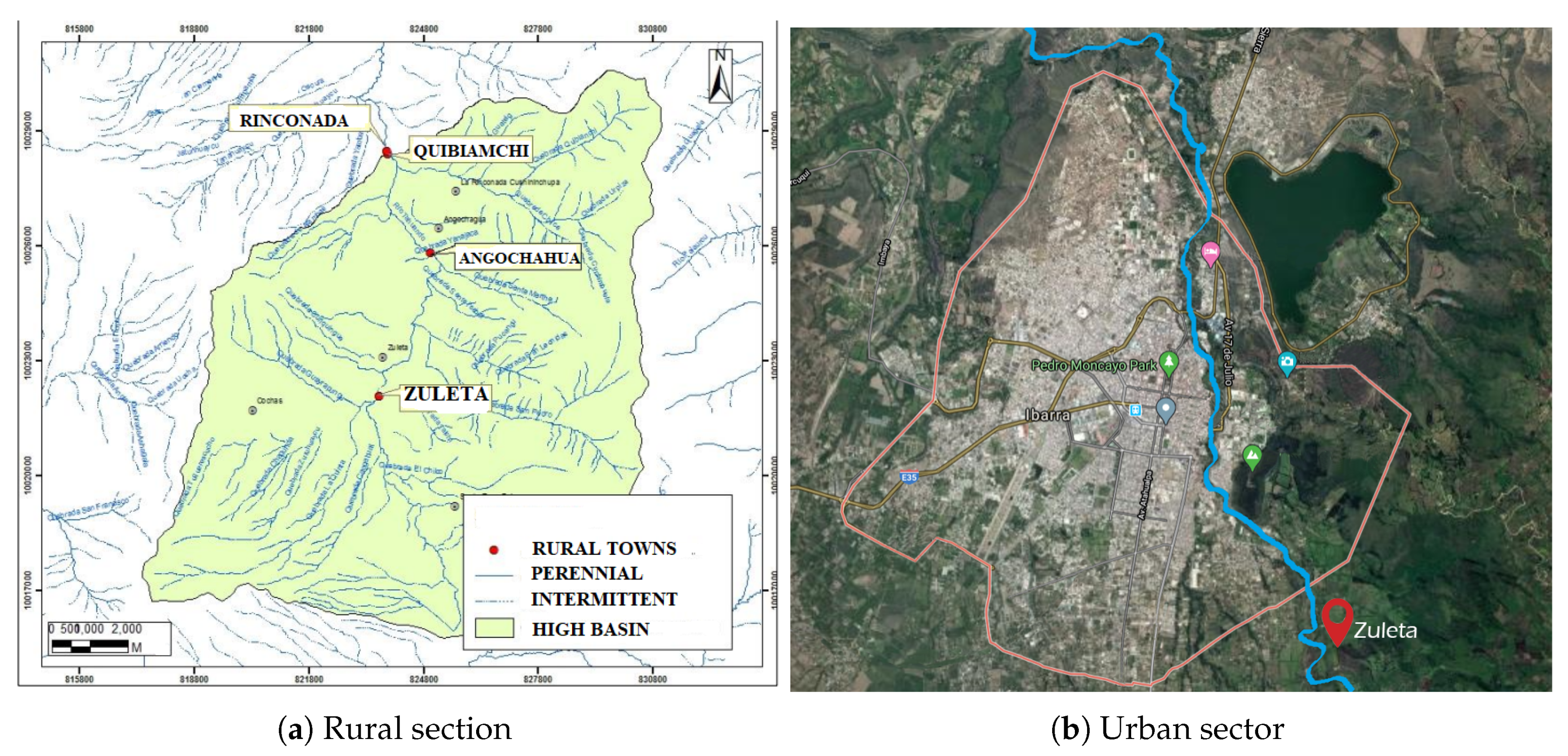
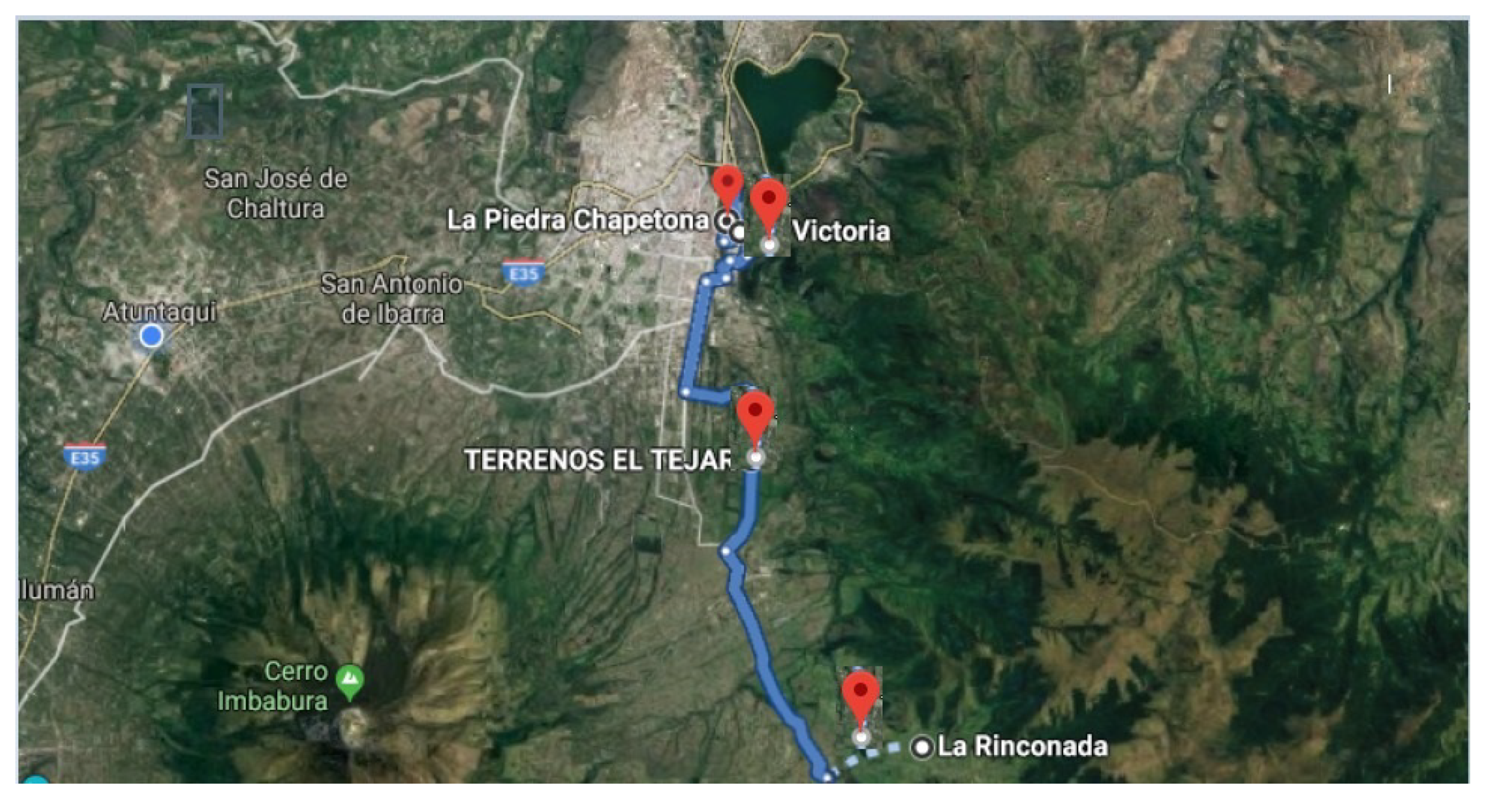
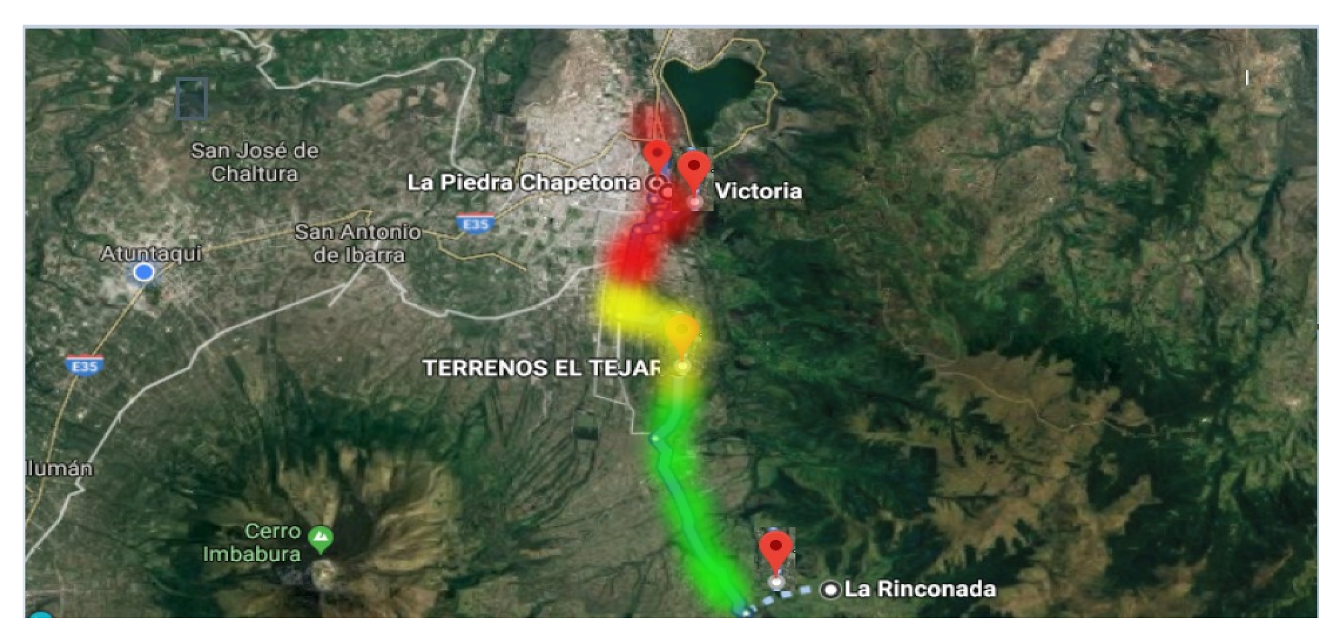
3.1. Initial Conditions of the Study Region

The city of Ibarra (Ecuador) is the capital of the province of Imbabura with a dry-temperate climate of 18 °C on average. The urban population is 109 thousand and a rural population of approximately 45 thousand inhabitants. Its main commercial activity is the production of wooden articles and services to medium-scale industries. Regarding its water supply, 90% is carried out through the public distribution network, while the rest is for the use of river and vertier water [24]. Tahuando river is an important water resource in the Imbabura province, being part of the natural system of Ecuador. Due to its ability to transport and the flowing of its waters, it can withstand a large number of pollutants. However, there are several modifications at the ecological level, such as the loss of aquatic species, foul-smelling, and watercolor changes, among others. In Ecuador, only $10\%$ of wastewater is treated. In Ibarra, around 600 liters per second of these waters are discharged into the Tahuando River, causing that no urban regeneration based on the increase in tourism can be carried out [25]. The Tahuando River is located at 0.4° latitude and 78.13° longitude. It encompasses an extension of 12 km from the community of Pesillo towards Salinas, in the Ibarra city. Figure 1 depicts the geographical location and basin.

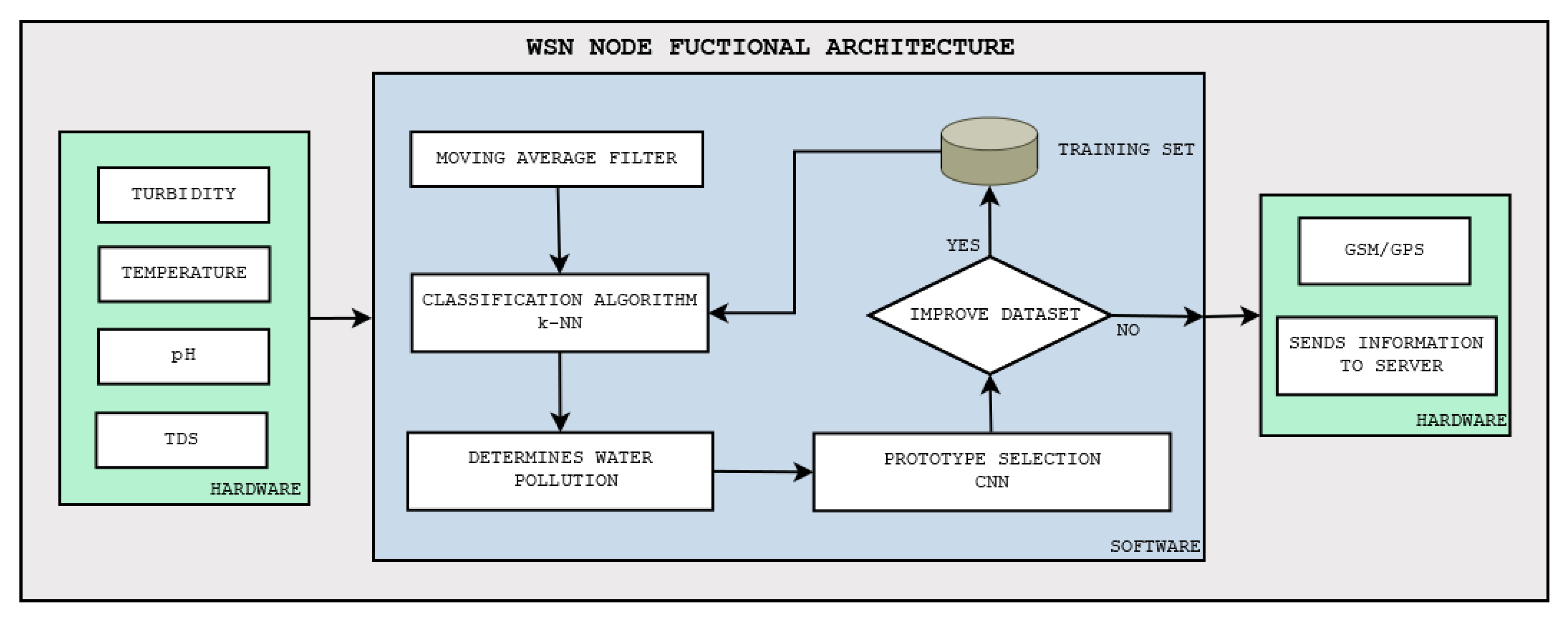
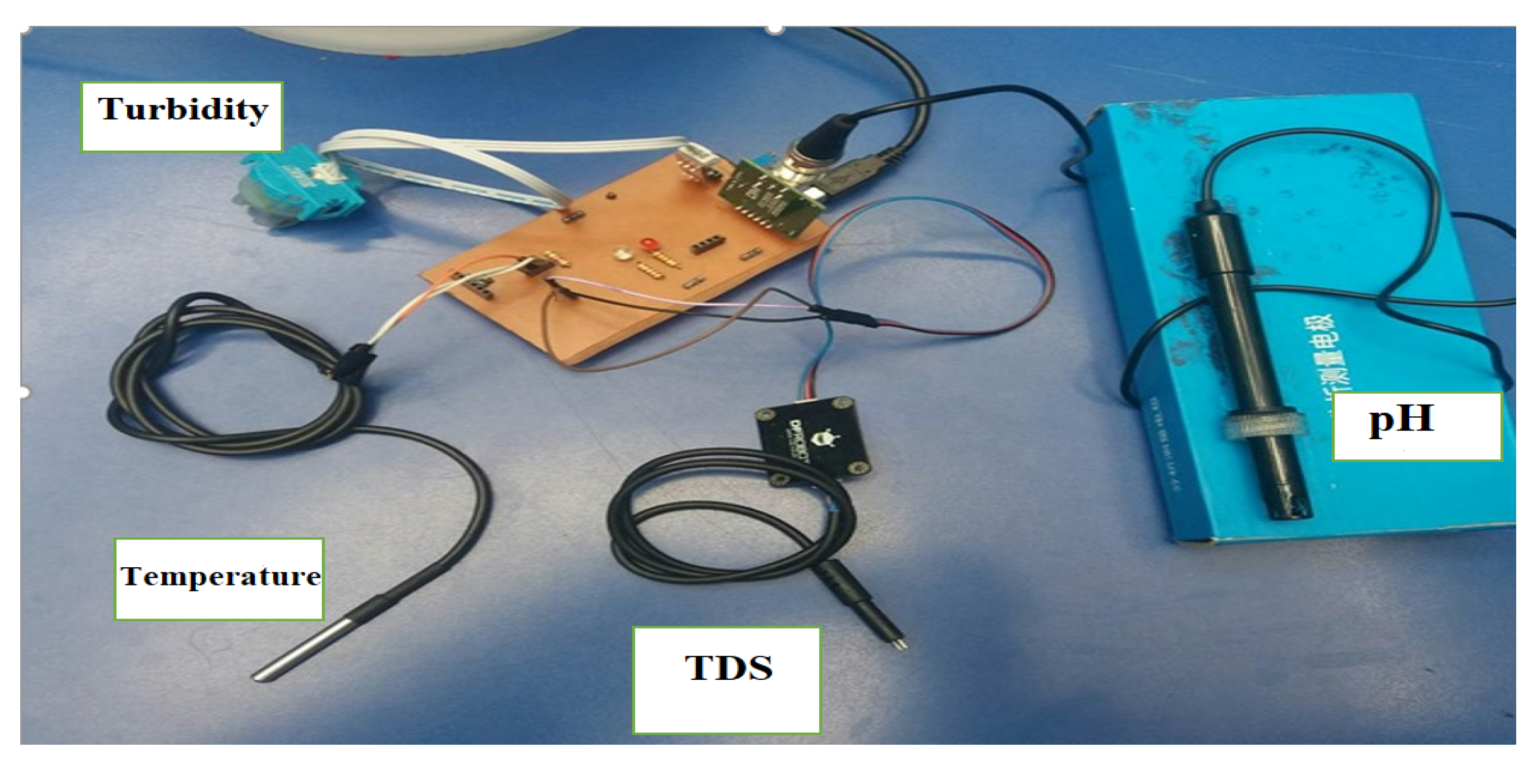
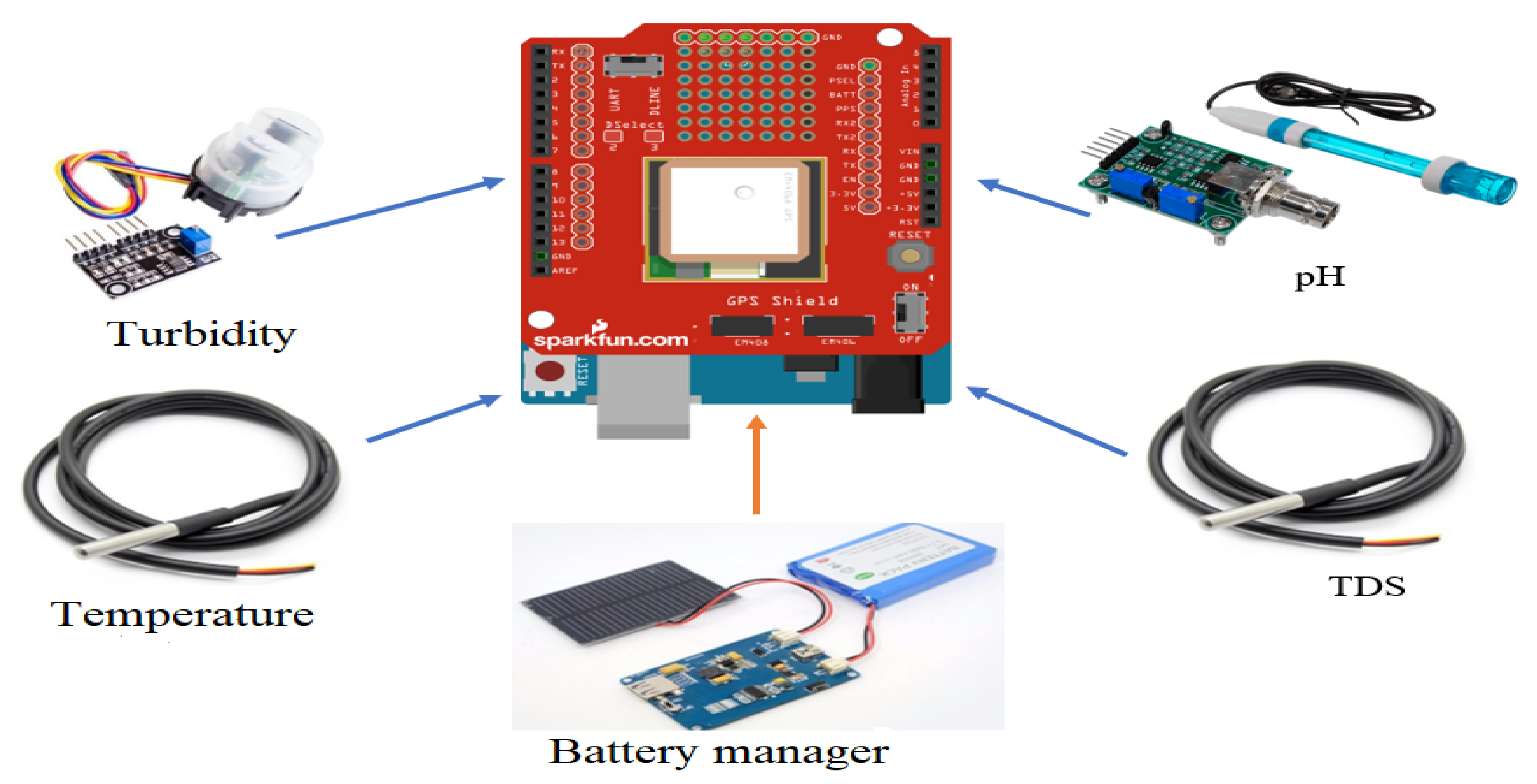
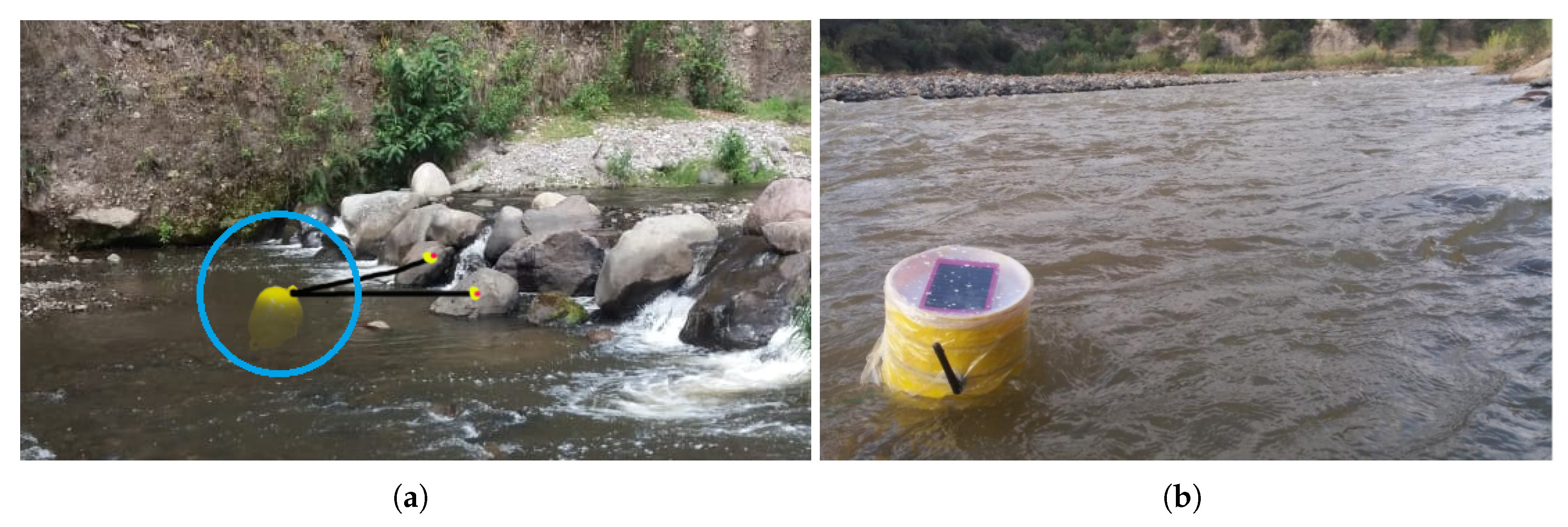
3.2. Wireless-Sensor-Network Design

The design of our WSN approach is followed from the considered water-quality-related variables: pH, turbidity, temperature and dissolved solids. The considered sensor network is as follows: Firstly, we measure the turbidity and identify what kind of pollutants can be found in the river, such as: wastewater, chemicals, among others. Secondly, we use a pH sensor to determine if the water composition is acidic or basic as well as a quality sensor (total dissolved solids, TDS) to assess the level of dissolved oxygen in the water (cleanliness) [9]. Thirdly, we incorporate a temperature sensor to determine the water’s changes and its relationship with the rest of the variables. To suitably develop the WSN network, we consider several operational requirements in the selection of sensors, such as reliability, precision, availability, ease-of-use, and scalability. Furthermore, in the selection of the WSN network processor system, we consider the number of pins and sensor libraries, as done in a previous work [11]. Specifically, the considered sensors are: SKU: SENO189 (turbidity), SKU: PH-7BNC (pH), Ds18b20 (temperature), RB-Dfr-797 (TDS). As well, the Arduino Uno is selected as processing system. Additionally, we use both global position module (GPS) and mobile communications (GSM) Sim808 to send data. Finally, there is a Lipo rider battery manager for power supply with a solar charging system. Figure 2 presents the considered sensors along with the processor system (Arduino Uno).

Likewise, we calibrate each sensor as follows: sensor SKU:PH-7BNC (pH) has a linear response, so its tuning is based on measuring the voltage of several pH solutions. Particularly, we use two solutions, the first one was pH = 4.01, getting a voltage of 2.98 volts; meantime, the second one was pH = 6.86, obtaining a voltage of 2.53 v. Thus, the equation to obtain the estimated pH is:

$$\begin{array}{c}\hfill \mathrm{pH}=-5.65\ast \left(v_1\right)+21.15,\end{array}$$

(1)

with $v_1$ as the voltage obtained by the sensor SKU:PH-7BNC. Likewise, the turbidity sensor SKU: SENO189 gives a reading ranging between 2.5 to 4.3 volts with values between 3000 and 0 turbidities (NTU), respectively. According to its datasheets, we can write the following equation:

$$\begin{array}{c}\hfill \mathrm{NTU}=-1120.4\ast {v_2}^2+5742.3\ast v_2-4352.9,\end{array}$$

(2)

where $v_2$ is the voltage registered by the sensor SKU:SENO189. On the other hand, the datasheet of the temperature sensor Ds18b20 indicates that each Celsius degree can be transformed using the equality 10 mv = 1 °C; thus, the equation is:

$$\begin{array}{c}\hfill Temp=\frac{v_3\ast 5}{1023\ast 0.01},\end{array}$$

(3)

with $v_3$ as the voltage obtained by the sensor Ds18b20.

Finally, the TDS RB-Dfr-797 sensor provides a flexible calibration protocol, with a reset button, we can return to the initial conditions, that is, a TDS value of 23 mv. Consequently, we refresh the Arduino program and use the next equation:

$$\begin{array}{c}\hfill \mathrm{TDS}=\frac{(30\ast 5\ast 1000)-(75\ast v_4)\ast 5\ast (1000/1024)}{75-0.23},\end{array}$$

(4)

where $v_4$ is the voltage obtained by the sensor RB-Dfr-797.

Upon sensor configuration, each $v_i$ value will correspond to a digital-analog converter (DAC) with a resolution of 10 bits, already in the microprocessor Arduino Uno. Furthermore, we implement the moving average recursive filter to reduce the acquisition errors and smoothing the signal from each DAC. This filter takes a subset (window) of N samples, and calculate its arithmetic average to estimate a filtered sample as [26]. This filter is implemented in each DAC separately through the following equation:

$$\begin{array}{c}\hfill y_n={(2n+1)}^{-1}\sum _{i=n-d}^{n+d}{x}_i,\end{array}$$

(5)

where $\mathsf{x}=(x_1,\dots ,x_{L_x})$ is the input signal, $\mathsf{y}=(y_1,\dots ,y_{L_y})$ is the filtered signal, d is the window size, and $L_x$ and $L_y$ are respectively the input and filtered signal lengths. To accounting for a reduction of the computational resources usage, we experimentally define $d=11$.

With the aim of verifying the data obtained by each sensor and validating the reliability thereof, samples obtained from the river are taken to the Environment Services Laboratory of the Technical University of the North (Universidad Técnica del Norte (Universidad Técnica del Norte official web site: https://www.utn.edu.ec/web/uniportal/) from Ibarra-Ecuador, as they count on the technology and reagents to make comparison against the data obtained by the WSN. In this sense, following reliability criteria for each sensor, some recommended performance measures are considered, such as: (i) Accuracy: ability to provide the same reading by repeatedly performing the same experiment (standard deviation), (ii) Reproducibility: ability to reproduce the same results when modifying initial conditions of the experiment, and (iii) Stability: ability to produce the same output value in a long time. Overall obtained results are gathered in

Table 1. Sensor performance metrics.

	Sensors
Measure	SENO189 (turbidity)	PH-7BNC (pH)	Ds18b20 (temperature)	RB-Dfr-797 (TDS)
Precision	7 ±	3 ±	5 ±	5 ±
Reproducibility	It is necessary to wait up 2 s for calibration to be done	Adequate	Adequate	Some reading errors
Stability	Adequate	3 ±, variable for each test	Adequate	Adequate

, which correspond to 10 tests over controlled environments to assess the data stability. As can be appreciated, the collected data from the sensors exhibit an error average of 5% in contrast to the those generated at the laboratory—such an error is acceptable enough for implementation purposes.

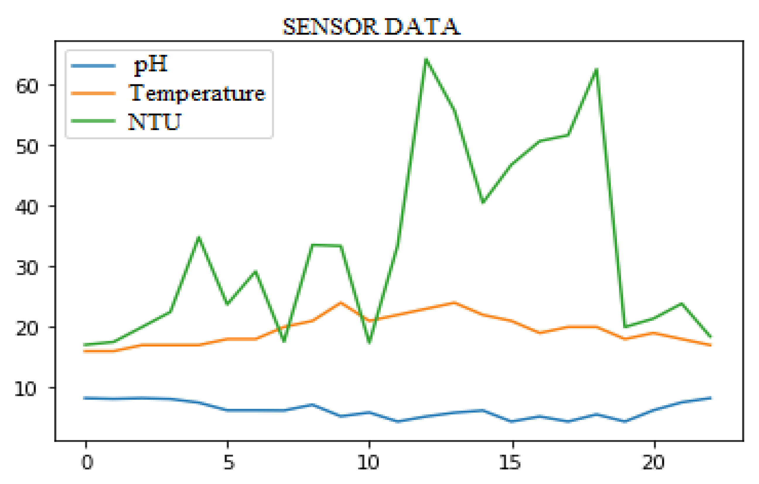
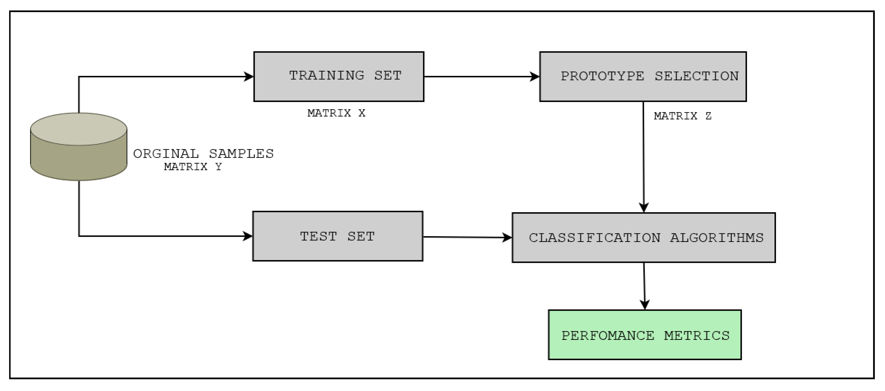
3.3. Data Analysis Paradigm

For a proper and wide data acquisition, we establish three node points in different locations, based on the population density of Ibarra, as follows: (i) La Rinconada, with low population and located at the river’s beginning; (ii) El Tejar, with middle population rate and some wastewater discharged into the river; and (iii) La Victoria, with a larger population density and more discharge of pollutants from the city. Figure 3 shows the geographic locations of the nodes. Furthermore, we label each data from the nodes with a localization tag. For the data acquisition procedure, we design a collection protocol as follows: A schedule consisting in four collecting times is set, namely: in the morning, afternoon, night and early morning. Such a schedule is timed with Timer2, which is an Arduino internal clock. So, the system is timed for alerts at 08:00, 12:00, 17:00 and 00:00. On those times, the system records the sensor readings every 10 min for two hours (amounting to 6 samples per hour). Finally, these captured data are sent to the remote server through the GSM/GPS sensor. This collection protocol was performed during 3 months, generating an enough amount of information to be used in the subsequent data analysis stage.

Once the data are stored in an external server, a two-stages data analysis process is carried out: The first stage is the training set size reduction—via prototype selection—involving the least or no affectation to the intrinsic knowledge they hold. The second one is the classification task, in which the the algorithm that best fits the first stage while keeping a high accuracy is sought. Both stages are set and performed under low-computational cost criteria (given the device conditions). This process is carried out in order to be compiled within each WSN node (including both prototype selection, and classification). Then, system is able to make their own decisions based upon the reduced, stored dataset as well as the implemented classification algorithm. Therefore, on the one hand, the adaptability criterion required by an intelligent system is met, by making it able to be used anywhere on the river. On the other hand, the resulting system requires no re-run the data analysis process and thus it can be readily used by any system operator whom is not required to hold an expertise on embedded systems or data analysis, but only knowledge in water treatment itself.

3.3.1. Proposed Quality Measure: Quantitative Metric of Balance (QMB)

Algorithm analysis is an important part of designing thereof. Traditionally, the analysis of programming code or algorithms lies in applying theoretical and mathematical procedures. Indeed, when selecting supervised classification algorithms, efficient programs must be ensured to be created, as this translates into better power consumption and therefore battery life time usage. In this sense, the here-introduced Quantitative metric of balance (QMB) is aimed at quantifying how proper is the ratio between classifier performance and the data size reduction by the prototype selection stage. In this connection, the closer its value is to $100\%$, the better the ratio. As these three individual measures have an increasing nature, we multiply them to state a single value, namely, the rate of removed instances ($RI$) times the classification performance ($CP$), and divided by the response time of the classification algorithms ($RT$), as follows:

$$\begin{array}{c}\hfill \mathrm{QMB}=\frac{(RI\ast CP)}{RT}\ast 100\%.\end{array}$$

(6)

Certainly, some classification criteria make use of mathematical functions or recursive functions of model adjustment that, when coded in a low-level language (assembler), generate response time delays, memory saturation and an excessive battery consumption. In this sense, the proposed QMB is aimed at penalizing the excessive computational cost in order to make it more feasible the implementation of data analysis algorithms into an embedded system. Besides, since it takes into consideration the number of removed training set instances to quantify the overall performance, this metric rewards the classification algorithm if it requires the least memory capacity when performing the decision-making procedures. When operating under real conditions, the system acquires the data from the sensors, filter the acquisition errors, make the decision through its compiled classification algorithm, and use the selection of prototypes to determine if this new reading improves the prediction ability of the system. If so, it is added into the training matrix otherwise it is only sent to the external server for visualization purposes.

Figure 4 shows the proposed data analysis scheme.

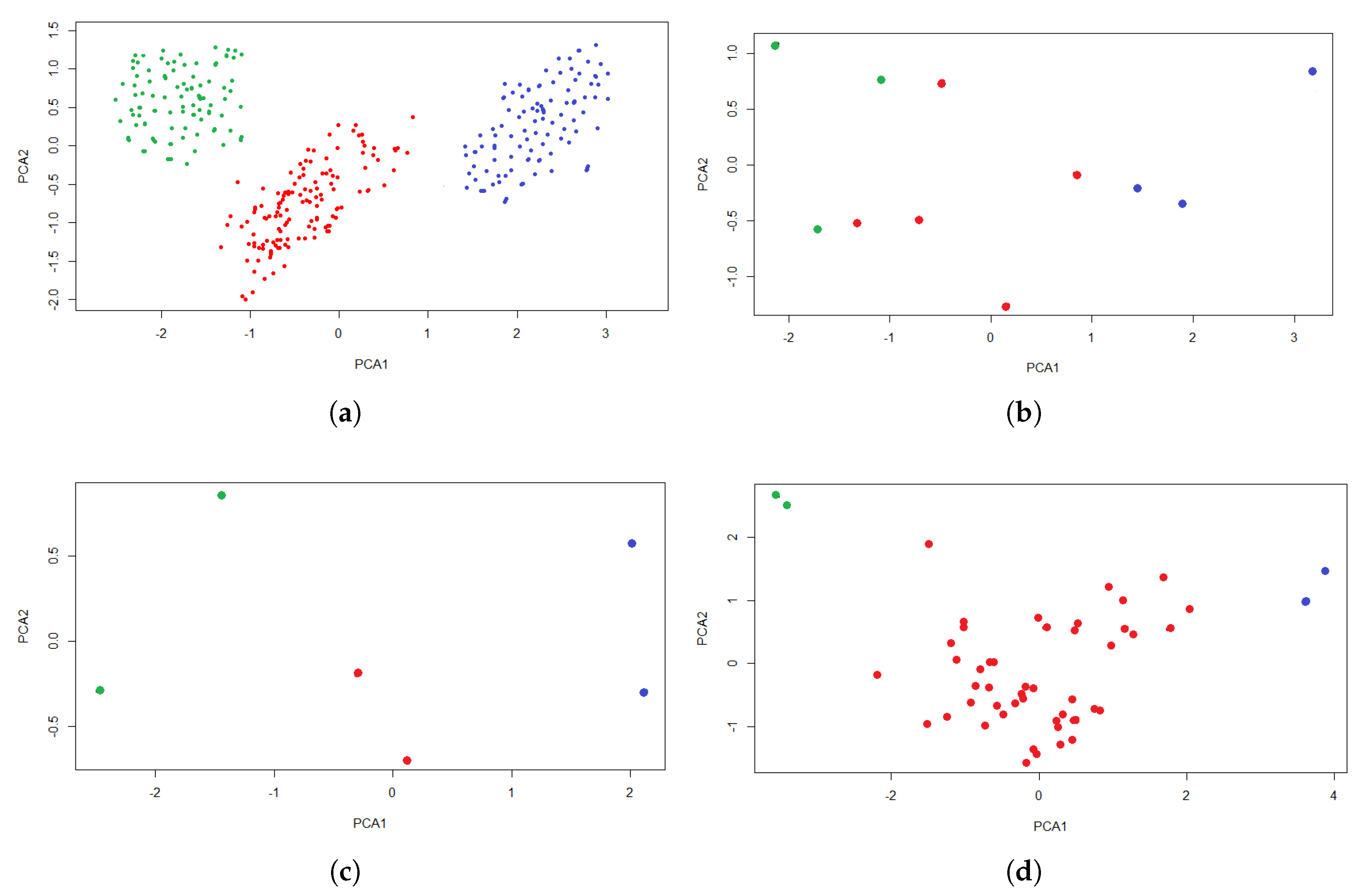
3.3.2. Prototype Selection

Since WSN systems have limited computational resources, its battery consumption is directly related to the amount of data to be processed, and therefore the implementation of machine learning algorithms into thereof is limited. In this connection, the prototype selection (PS) techniques may take place by reducing the training matrix size, while utmost maintaining as good classification performance as that obtained when considering the original size. Regarding PS algorithm designing, technical literature reports at least three main methods (namely, compensation-based, edition-based, and hybrid) [27]. As have been mentioned throughout this paper, the whole process is carried out in such manner that the prototype selection results (reduced data matrices) can be stored directly into every WSN node.

In this work, in order to account for an enough coverage, we have chosen three representative algorithms of each method, as follows:

• Condensation: Condensed Nearest Neighbor (CNN), Reduced Nearest Neighbor (RNN), and Selective Nearest Neighbor (SNN).
• Edition: Edited Nearest Neighbor (ENN), All-k Edited Nearest Neighbors (AENN), and Iterative Partitioning Filter (IPF).
• Hybrid: Decremental Reduction Optimization Procedures 2 (DROP 2), Decremental Reduction Optimization Procedures 3 (DROP3), and Iterative Noise Filter based on the Fusion of Classifiers (INFFC).

3.3.3. Classification Algorithms

Classification algorithms can learn based on different criteria, having each of them representative algorithms [27]. Herein, we consider four criteria and their respective representative algorithm, namely:

• Distance-based: K-Nearest Neighbors (KNN).
• Model-based: Support Vector Machine (SVM).
• Density-based: Bayesian classifier (BC).
• Heuristic: Decision Tree (DT).

Given that the four aforementioned criteria are essentially different, a comparison of individual performances is necessary to identify the one(s) best fitting the nature of data and classification task. As well, it is of crucial interest to measuring the computational cost that each algorithm involves to be further implemented within the WSN node.

The database—obtained according to the pollution level—has been divided regarding the information acquired by the WSN nodes into 3 types (being our training labels): high, medium and low contamination. Therefore, if the system is located at different spots along the river, it can generate a map of the pollution status and estimate the river’s course. Alternatively, if it is located statically, the system can determine, in hours, how the level of contamination varies with respect to the time of day.

4. Results and Discussion

In order to evaluate the behavior of each stage, we firstly discuss the data reduction in the training matrix. Subsequently, we show the outcome of our proposed analysis scheme, namely, the performance analysis using our defined metric (QMB) for determining the ideal algorithms for its implementation in the WSN nodes. Finally, we present the results of the final implementation of the system and the tests in real environments.

4.1. Data Reduction

The sensors were acquiring data during the months of July, August and September on random days. As a result, we obtained the data matrix called $\mathsf{Y}\in {\mathbb{R}}^{m\times n}$, where m is the number of instances, and n the number of measured variables (sensors). While, $\mathsf{L}\in {\mathbb{R}}^{m\times 1}$ is the tag vector. Thus, we have that $m=507$, and $n=4$. With these data, we implemented the PS algorithms in order to reduce the training matrix and processing time. In addition, to validate the classification criteria, we retained 20% of the $\mathsf{Y}$ matrix for performance testing. In succession, the matrix for the data scheme is $\mathsf{X}\in {\mathbb{R}}^{p\times n}$, where $p=405$.

Table 2. Analysis of PS algorithms in relation to optimization embedded computational resources.

PS Algorithm	Exec. Time (s)	Remv. Inst	% of Remv. Inst
AENN	3.17	0	0
BBNR	125.23	102	25.18
CNN	2.28	394	97.28
DROP1	130.63	399	98.51
DROP2	230.28	354	87.407
DROP3	264.97	354	87.40
ENG	250	210	51.85
ENN	0.72	0	0
RNN	2.39	394	97.28

shows the summary of the PS algorithms results and find a new reduced data matrix $\mathsf{Z}$.

Accordingly, we have selected the CNN, DROP1 and DROP3 algorithms as they reach the highest percentages of reduction in the database. Figure 5 shows scatter plots of the initial data set and the reduced versions generated by CNN, DROP1 and DROP3.

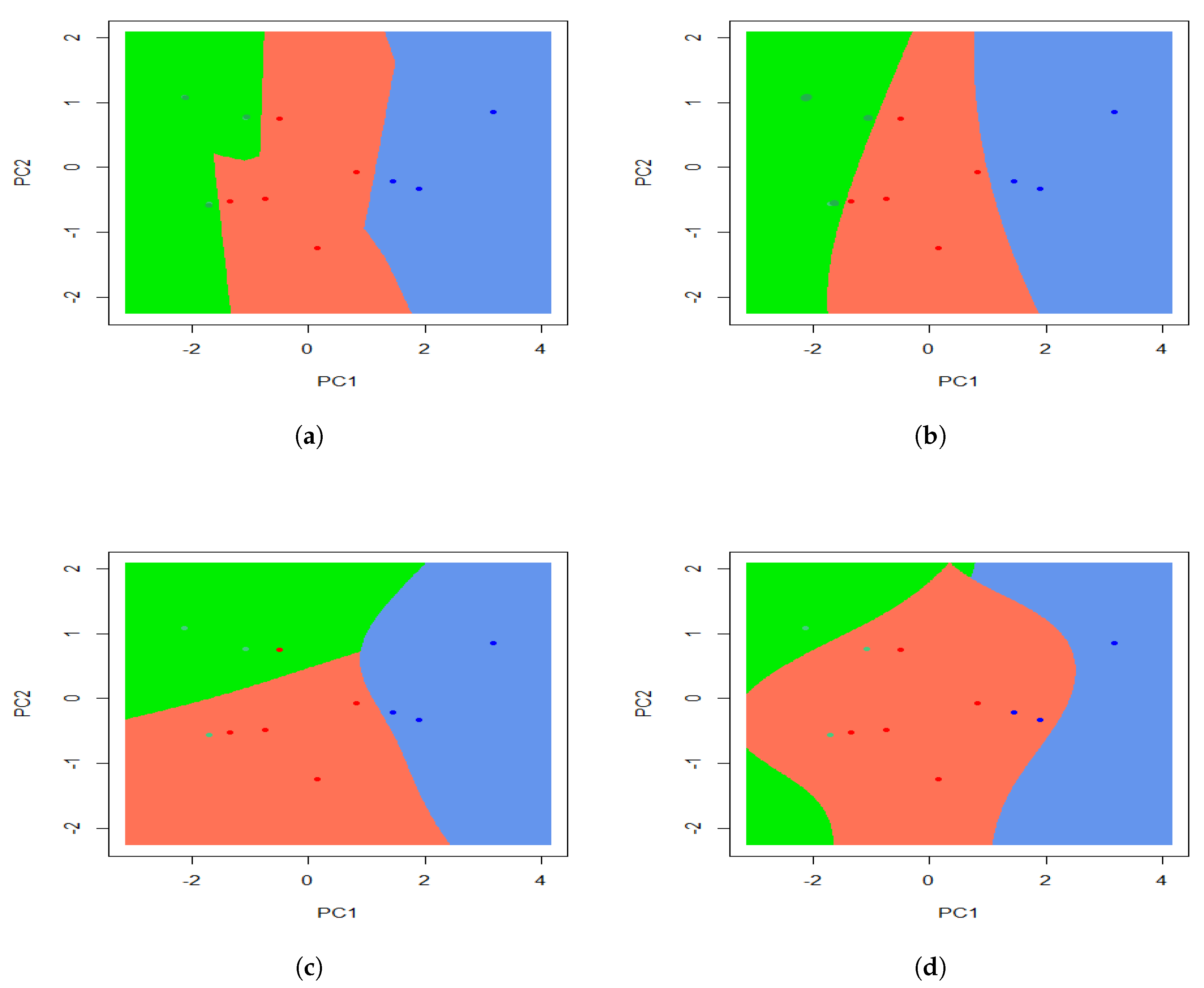
4.2. Classification Performance

With the reduced data sets, we compared the classification performance using the aforementioned algorithms.

Table 3. Classifier’s metrics.

Classifier	Matrix X%	CNN%	DROP1%	DROP3%
Accuracy
k-NN	97.6	90.6	93.6	95
Bayesian classifier	95	87.5	82.6	0.99
Decision Trees	99.3	66.9	33.33	33.33
SVM (Polynomial kernel)	100	75	75.3	92.14
SVM (Sigmoide kernel)	100	75	92	100
Sensitivity
k-NN	96.6	88.3	91.6	93.3
Bayesian classifier	93.3	75	76	97.3
Decision Trees	99.3	33	33.33	33.33
SVM (Polynomial kernel)	100	94	66.9	92.14
SVM (Sigmoide kernel)	100	50	90	100
Specificity
k-NN	98.2	93.6	95.3	96.6
Bayesian classifier	96.6	88.6	88	99.3
Decision Trees	99.6	66.9	33.33	33.33
SVM (Polynomial kernel)	100	97	89	100
SVM (Sigmoide kernel)	100	100	94	100
Precision
k-NN	96.3.0	98.3	89.3	93.3
Bayesian classifier	93.3	100	66.6	98.3
Decision Trees	93.3	33.9	33.33	33.33
SVM (Polynomial kernel)	100	93	89	93.13
SVM (Sigmoid kernel)	100	50	86.6	100

summarizes the results of the classifiers with cross-validation with ten random folds.

To graphically appreciate the results of the whole data processing scheme, just as done in previous works [11,14], we use the principal component analysis conventional algorithm as a dimensionality reduction approach to represent the original data over a lower-dimensional domain. Figure 6 presents scatter plots regarding the two first principal components to depict the decision borders generated by every considered classifier. This process is carried out for demonstration purposes in order to know the algorithms’ ability to differentiate each label in an understandable way for the human being perception (visual-type in this case).

Numerical results of the joint performance of the prototype selection and data classification are summarized in

Table 4. QMB analysis for every classifier along with the previously identified PS algorithms.

Classification	Exec. Time (s)	QMB Value
algorithm		CNN%	DROP1%
k-NN	1.21	72.85	76.20
Bayesian	1.85	46.01	43.97
Decision Tree	0.77	42.06	42.63
SVM (polynomial kernel)	5.2	14.03	14.2
SVM (sigmoide kernel)	6.1	11.96	12.11

.

Discussion on performance measures: As can be seen in the Table 3, VSM reaches the best classification performance based on the considered metrics (100%). Nonetheless, its algorithm involves mathematical functions (known as kernel functions), which are not able to readily processed in a WSN. In this connection, the proposed QBM allows for warning about this computational cost in relation to the amount of data used to train the classification algorithm and the system response time when assigning the corresponding label to a new data from the sensors. This can be appreciated from the fact that by reducing the training matrix its performance decreases significantly. The same occurs for all the considered algorithms excepting for k-NN, whose distance-based nature is non-expensive in terms of computational cost. Furthermore, by using a reduced data matrix, k-NN considerably maintains its performance. Furthermore, it is clearly noted that DROP1 is the best-suited algorithm for prototype selection although its computational cost is very high. Hence, given the design settings and the embedded systems conditions, CNN is preferred and therefore selected as the algorithm for prototype selection, while k-NN is considered as the selected classification algorithm reaching a performance of 90.6% and a QBM value of 72.85%.

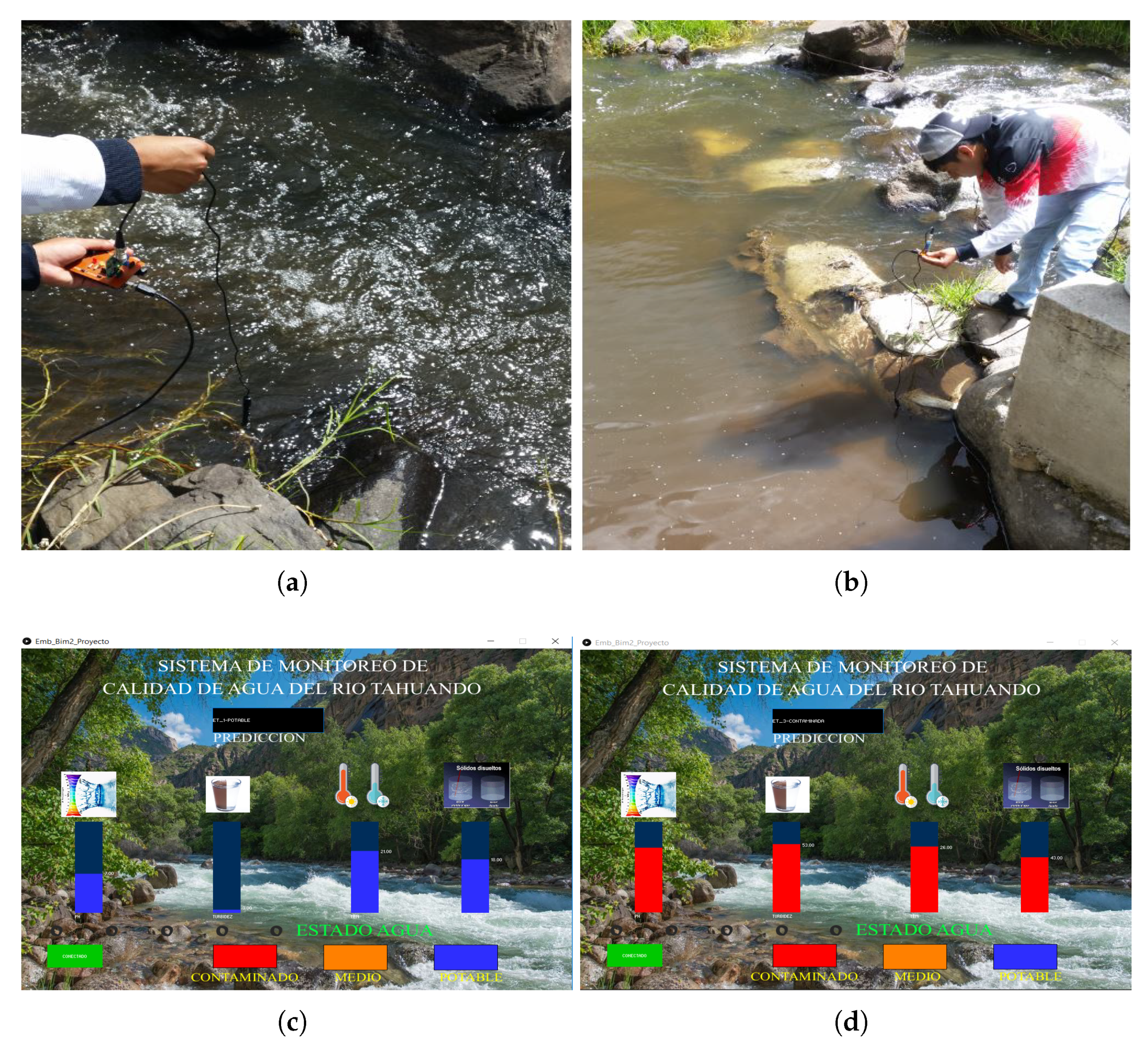
4.3. Implementation and Testing

Figure 7 depicts the functional architecture of the nodes using the proper, selected prototype selection algorithms, which are to be compiled within thereof. As can be appreciated, each node holds the data-acquisition sensor set. The data analysis and processing is as follows: The raw data is first filtered by using the Moving average filter, which, in this case, is enough to remove the components (artifacts) related to reading errors and noise. Subsequently, data are classified by the algorithm k-NN, which assigns a label and decides about the predicted level of water contamination according to the training database and following a distance-based, majority-vote-driven approach. Then, data undergo an additional processing via CNN to determine whether the training database can be improved by removing instances exhibiting negligible relevance regarding either the subsequent classification task or the intrinsic knowledge they may hold. Finally, the output information is converted into a character string together with its label to be sent by the GSM network to the external server and display the data obtained from each sensor and the decision made. It is worth highlighting that the node to be monitored can be selected through the interface.

In the overall work-flow of our approach, the need for using an external sever lies in the fact that optimizing resource consumption at the in-situ analysis (directly on WSN Nodes) entails performing offline data processing tasks, mainly, at three specific points. The first one is when collecting data from each WSN node, being its main function the storing of such information (which—at this extent—corresponds to the outcomes of reading-errors-filtering stage produced by the moving average filter). The second one is the offline, exhaustive running, and comparison of classification algorithms to identify the ones reaching a good compromise between accuracy and computational cost, and therefore, being adequate to be directly implemented into the WSN nodes. Finally, as the third point, the server is used for information visualization purposes (displaying numerically and graphically the acquired data, the decision (classification) made by each node and the river pollution historical). This information is also stored in the server. Of course, those algorithms identified as adequate ones at the second point are the ones that are finally incorporated into the WSN nodes.

Once performed the data analysis procedures, we integrate all sensors into a PCB board incorporating an Arduino Uno as a processor unit. A view of the developed WSN node can be seen in Figure 8.

The developed WSN has a considerably high operating consumption for a LiPo-type battery. To increase the life time of both the system and the battery, energy saving modes are used inside the Arduino board that handles the sensor activation. To enable such modes, we consider the use of timers, which work as an internal clock determining the data-acquisition-and-sending timing, and therefore limit current consumption. Hence the power consumption of every single sensor and the processor should be considered. In normal operation conditions, the total electric current consumption (considering all the sensors) amounts to 110 mA, while the GPS-GSM module and the Arduino require 40 mA and 45 mA, respectively. Meanwhile, when the battery saving system is enabled, the sensors and the GPS module are not is used, and thus only the Arduino works and is fed with 15mA. As stated in [28], the following equation relates the battery life time with the total power consumption (P):

$$P=\frac{(T_{on}\ast I_{on})+(T_{sleep}\ast I_{sleep})}{T_{on}+T_{sleep}},$$

(7)

where $T_{on}$, $T_{sleep}$, $I_{on}$, and $I_{sleep}$ stand respectively for Normal Consumption Time, Sleep Consumption Time, Current Consumption at Normal Conditions, and Current Intensity Sleeping Consumption.

As explained in Section 3.3, the system is on during 10 min and then remains in battery saving mode. As a result, the system consumes 78.45 mA per hour. If the used battery is 5 volts at 1000 mA, the system can work continuously for 12.73 h. However, the system is activated only four times per day (early morning, mid-morning, afternoon and night), that is, it only works for 4 h a day. As a result, the system can remain for at least 3 days with no requiring battery manager support. As an advantageous aspect of our system we may say that, when implemented with a solar panel powering the battery, there is experimental evidence that it can work up to 4 months with no discharging or critical battery issues.

Subsequently, over the implemented system, we store the training dataset obtained after running the CNN algorithm, which is to denoted $\mathsf{Z}\in {\mathbb{R}}^{s\times n}$, by setting the number of prototypes as $s=11$. At this extent, CNN algorithm is considered as an recommendable approach, since its execution time is the least while its ability to reduce the dataset instances is proper enough. Consequently, if the system requires to be reconfigured to train the classification algorithm model, the CNN algorithm can be compiled readily on the WSN network with no entailing extra battery consumption or diminishing the system performance. Then, we implemented the Bayesian classifier so that it can make system decisions concerning the tag assigned by location. Thus, we can determine the contamination levels (high, medium, low) using the nodes along the river. Since the system is intended to be waterproof, we use a river buoy to keep the system afloat. At its upper part, we install the solar panel and the GPS-GSM communication antenna. Furthermore, the nodes are anchored using an ironwork attached to the river stones, as shown in Figure 9.

Besides, for displaying purposes, we develop a monitoring interface in Processing using a local server that downloads and visualizes the information from the server. In this interface, we show the status of each sensor, the node location, and the level of contamination of the river. Figure 10 summarizes both the sensor testing and the visual interface with the decision taken.

For a more extensive analysis, we move the nodes throughout the river to assign a color label, based on the contamination level, as follows: red refers to high contamination, yellow to medium, and green to null or low pollution. Accordingly, Figure 11 shoes the contamination levels along the case-study river. As a relevant result, we identify that at the Campiña church zone there is already a high level of pollution.

Finally, with all nodes running, we daily capture data to observe the maximum values, in order to detect the hours of the day with highest contamination, which are in line with the human’s work schedules. Figure 12 shows the pH, Temperature, and NTU values registered by the sensors during a whole day.

It is worth mentioning that our system may exhibit failures regarding the loss of signal from the GPS-GSM module when restarting it to carry out the data acquisition. To overcome this drawback, we follow a heuristic sensor calibration procedure as follows: On one hand, when activated, the system first turns on the GPS-GSM module so that there would be enough time to re-link to the GSM network and send back a status indicator signal. On the other hand, the length of the cables connected to the sensors was initially very long. This caused that when the volume of water decreased, cables descended to the bottom of the river and got brushed against stones. Consequently, since the length of the system-incorporated sensor is between 2 and 5 cm, an excessive wear on the sensors is induced. To cope with this issue, we search for and identify points where the river depth is the least possible varying, and is not prone to water stagnation.

5. Final Remarks

In this work, we present the complete design and validation of an intelligent wireless sensor network (WSN) system to measure the contamination levels of a river. Particularly, the Tahuando River is of interest. Broadly speaking, the proposed system involves two stages: electronic device implementation, and data analysis.

For the electronic design, since the case-study river may have high levels of pollution, as well as it may occur significant variations depending on the hours of the day, and zones of its route, we implement several WSN nodes for acquiring the river’s conditions information by covering a meaningful zone and within a wide enough range of time. In this sense, we both calibrate and tune the sensors for a correct data collection. Additionally, we experimentally demonstrate that our data reading schedules were adequate for detecting higher pollution hours. Furthermore, we highlight that the river buoys is a key element to meet the node’s permeability requirements as well as to enable the proper functioning of each WSN node.

Regarding the proposed data analysis scheme, we demonstrate that a classifier together with a prototype selection is suitable for a WSN-based water-quality monitoring system. It is reached a good trade-off between the computational resource usage (as the training matrix size is reduced to meet the system operation conditions), and the classification performance at detecting the pollution levels along the river. In addition, given the network coverage, the proposed system is able to send information from the WSN node to the server. Therefore, the filtered data can be visualized in an interface, and an in-situ analysis becomes possible. It is important to mention that the server is only for data visualization purposes and does not have the implementation of machine learning algorithms.

As a future work, the battery life is to be more carefully considered by exploring both different methods of extending its duration and alternatives sources of energy to supply the nodes (i.e., using the water flow to generate energy). A large number of nodes and wider coverage (located at different water resources around the province of Imbabura, Ecuador) is highly desirable for further In addition, we are intended to a seek for alternatives to mitigate system affectations due to disturbances caused by the presence of unexpected individuals (either people or animals), as so far our readily solution has been to locating the system in a hardly visible and difficult-to-access spot.

References

1. Venancio Cruz, D.; Rivelino Gomes de Oliveira, M.; Cunha Filho, M.; Venancio da Cruz, D. Monitoring pH with quality control based on Geostatistics Methodology. IEEE Lat. Am. Trans. 2016, 14, 4787–4791. [Google Scholar] [CrossRef]
2. Yang, C.; Wang, X. The water quality and pollution character in QingShuiHai lake valley-typical urban drinking water sources. In Proceedings of the 2011 International Conference on Remote Sensing, Environment and Transportation Engineering, Nanjing, China, 24–26 June 2011; pp. 7287–7291. [Google Scholar]
3. Zhang, Z.; Zhang, F.; Xu, C.; Xu, J.; Zhang, W.; Qi, Q. Study on the water environment capacity for the typical watershed in Taizihe River. In Proceedings of the 2011 International Symposium on Water Resource and Environmental Protection, Xi’an, China, 20–22 May 2011; Volume 1, pp. 486–488. [Google Scholar]
4. Randhawa, S.; Sandha, S.S.; Srivastava, B. A Multi-sensor Process for In-Situ Monitoring of Water Pollution in Rivers or Lakes for High-Resolution Quantitative and Qualitative Water Quality Data. In Proceedings of the 2016 IEEE Intl Conference on Computational Science and Engineering (CSE) and IEEE Intl Conference on Embedded and Ubiquitous Computing (EUC) and 15th Intl Symposium on Distributed Computing and Applications for Business Engineering (DCABES), Paris, France, 24–26 August 2016; pp. 122–129. [Google Scholar] [CrossRef]
5. Zhai, C.; Huang, Q.; Chang, J.; Gao, F. The study of water resources reasonable allocation of BaoJi area in Wei River with considering the ecology base flow. In Proceedings of the 2011 International Symposium on Water Resource and Environmental Protection, Xi’an, China, 20–22 May 2011; pp. 816–818. [Google Scholar] [CrossRef]
6. Guo, W.; Chen, J.; Sheng, Y.; Wang, J. Integrated evaluation of water quality and quantity of the Wei River reach in Shaanxi Province. In Proceedings of the 2011 International Symposium on Water Resource and Environmental Protection, Xi’an, China, 20–22 May 2011; pp. 863–866. [Google Scholar] [CrossRef]
7. Zhang, H.; Xie, X.; Hou, J. Water pollution accident control and urban safety water supply. In Proceedings of the 2011 2nd IEEE International Conference on Emergency Management and Management Sciences, Beijing, China, 8–10 August 2011; pp. 37–40. [Google Scholar]
8. De Agua, S. Biblioteca—Secretaría del Agua. Available online: https://www.agua.gob.ec/ (accessed on 1 January 2020).
9. Wang, J.; Guo, X.; Zhao, W.; Meng, X. Research on water environmental quality evaluation and characteristics analysis of TongHui River. In Proceedings of the 2011 International Symposium on Water Resource and Environmental Protection, Xi’an, China, 20–22 May 2011; pp. 1066–1069. [Google Scholar] [CrossRef]
10. Taufiqurrahman; Tamami, N.; Putra, D.A.; Harsono, T. Smart sensor device for detection of water quality as anticipation of disaster environment pollution. In Proceedings of the 2016 International Electronics Symposium (IES), Denpasar, Indonesia, 29–30 September 2016; pp. 87–92. [Google Scholar] [CrossRef]
11. Rosero-Montalvo, P.D.; Pijal-Rojas, J.; Vasquez-Ayala, C.; Maya, E.; Pupiales, C.; Suarez, L.; Benitez-Pereira, H.; Peluffo-Ordonez, D. Wireless Sensor Networks for Irrigation in Crops Using Multivariate Regression Models. In Proceedings of the 2018 IEEE Third Ecuador Technical Chapters Meeting (ETCM), Cuenca, Ecuador, 15–19 October 2018; pp. 1–6. [Google Scholar] [CrossRef]
12. Ragnoli, M.; Barile, G.; Leoni, A.; Ferri, G.; Stornelli, V. An Autonomous Low-Power LoRa-Based Flood-Monitoring System. Low Power 2020, 10, 15. [Google Scholar] [CrossRef]
13. Alippi, C. Intelligence for Embedded Systems; Springer: Berlin/Heidelberg, Germany, 2014; pp. 1–283. [Google Scholar] [CrossRef] [Green Version]
14. Rosero-Montalvo, P.D.; Batista, V.F.L.; Rosero, E.A.; Jaramillo, E.D.; Caraguay, J.A.; Pijal-Rojas, J.; Peluffo-Ordóñez, D.H. Intelligence in Embedded Systems: Overview and Applications; Springer: Cham, Switzerland, 2019; pp. 874–883. [Google Scholar] [CrossRef]
15. Guo, M.; Zhou, X. Research on the water environment capacity of Chanba River downstream. In Proceedings of the 2011 International Conference on Electric Technology and Civil Engineering (ICETCE), Lushan, China, 22–24 April 2011; pp. 4411–4414. [Google Scholar] [CrossRef]
16. Patel, H.J.; Dabhi, V.K.; Prajapati, H.B. River Water Pollution Analysis using High Resolution Satellite Images: A Survey. In Proceedings of the 2019 5th International Conference on Advanced Computing & Communication Systems (ICACCS), Coimbatore, India, 15–16 March 2019; pp. 520–525. [Google Scholar] [CrossRef]
17. Shukla, A.K.; Ojha, C.S.P.; Garg, R.D. Surface water quality assessment of Ganga River Basin, India using index mapping. In Proceedings of the 2017 IEEE International Geoscience and Remote Sensing Symposium (IGARSS), Fort Worth, TX, USA, 23–28 July 2017; pp. 5609–5612. [Google Scholar] [CrossRef]
18. Lin, Z.; Wang, W.; Yin, H.; Jiang, S.; Jiao, G.; Yu, J. Design of Monitoring System for Rural Drinking Water Source Based on WSN. In Proceedings of the 2017 International Conference on Computer Network, Electronic and Automation (ICCNEA), Xi’an, China, 23–25 September 2017; pp. 289–293. [Google Scholar]
19. Sowmya, C.; Naidu, C.D.; Somineni, R.P.; Reddy, D.R. Implementation of Wireless Sensor Network for Real Time Overhead Tank Water Quality Monitoring. In Proceedings of the 2017 IEEE 7th International Advance Computing Conference (IACC), Hyderabad, India, 5–7 January 2017; pp. 546–551. [Google Scholar]
20. Chen, F.; Wen, F.; Jia, H. Algorithm of Data Compression Based on Multiple Principal Component Analysis over the WSN. In Proceedings of the 2010 6th International Conference on Wireless Communications Networking and Mobile Computing (WiCOM), Chengdu, China, 14 October 2010; pp. 1–4. [Google Scholar]
21. Kadir, E.A.; Irie, H.; Rosa, S.L. River Water Pollution Monitoring using Multiple Sensor System of WSNs (Case: Siak River, Indonesia). In Proceedings of the 2019 6th International Conference on Electrical Engineering, Computer Science and Informatics (EECSI), Bandung, Indonesia, 18–20 September 2019; pp. 75–79. [Google Scholar]
22. Zhang, Z. Data Fusion Optimization Analysis of Wireless Sensor Networks Based on Joint DS Evidence Theory and Matrix Analysis. In Proceedings of the 2019 4th International Conference on Mechanical, Control and Computer Engineering (ICMCCE), Hohhot, China, 24–26 October 2019; pp. 689–6894. [Google Scholar]
23. Torres, A.J.; Quezada, M.; Carrion, L.; Coronel, I.; Barragen, A. AHP analysis to minimize the effects produced by the textile industry in the rivers of Cuenca city. In Proceedings of the 2017 IEEE Mexican Humanitarian Technology Conference (MHTC), Puebla, Mexico, 29–31 March 2017; pp. 94–101. [Google Scholar] [CrossRef]
24. De Estadística y sensos, I.N. Fasículo Provincial de Imbabura. Available online: https://www.ecuadorencifras.gob.ec/institucional/home/ (accessed on 1 January 2020).
25. Encarnación, D.; Enríquez, J.; Suarez, L. Derecho De La Naturaleza: Caso Rio Tahuando; Technical Report; Universidad Andina Simń Bolivar: Ambato, Ecuador, 2012. [Google Scholar]
26. Liu, J.; Deng, Z. Self-tuning weighted measurement fusion Wiener filter for autoregressive moving average signals with coloured noise and its convergence analysis. IET Control. Theory Appl. 2012, 6, 1899–1908. [Google Scholar] [CrossRef]
27. Rosero-Montalvo, P.D.; López-Batista, V.F.; Peluffo-Ordóñez, D.H.; Erazo-Chamorro, V.C.; Arciniega-Rocha, R.P. Multivariate Approach to Alcohol Detection in Drivers by Sensors and Artificial Vision. In From Bioinspired Systems and Biomedical Applications to Machine Learning; Ferrández Vicente, J.M., Álvarez-Sánchez, J.R., de la Paz López, F., Toledo Moreo, J., Adeli, H., Eds.; Springer International Publishing: Cham, Switzerland, 2019; pp. 234–243. [Google Scholar]
28. Antolín, D.; Medrano, N.; Calvo, B. Analysis of the operating life for battery-operated wireless sensor nodes. In Proceedings of the IECON 2013—39th Annual Conference of the IEEE Industrial Electronics Society, Vienna, Austria, 10–13 November 2013; pp. 3883–3886. [Google Scholar]
Figure 1. Geographical description of Tahuando river. Zoomed view of the river route highlighting remarkable surrounding communities in Ibarra city’s urban sector (right), and a widespread view regarding the rural section of Imbabura province (left).
Remotesensing 12 01988 g001
Figure 2. Demonstrative diagram of the proposed WSN system. Considered sensors (SKU: SENO189 (turbidity), SKU: PH-7BNC (pH), Ds18b20 (temperature), RB-Dfr-797 (TDS)), and the processor (Arduino Uno).
Remotesensing 12 01988 g002
Figure 3. Geographic location of the WSN nodes. Spots strategically selected to acquire data from, in order to encompass representative zones, as well as different types and levels of river pollution.
Remotesensing 12 01988 g003
Figure 4. Data analysis scheme including prototype selection and classification stages.
Remotesensing 12 01988 g004
Figure 5. 2D scatter plots of resulting data matrices Z of the chosen prototype selection algorithms. (a) Data matrix X, (b) CNN, (c) DROP1, (d) DROP3.
Remotesensing 12 01988 g005
Figure 6. Decision borders for each classifier. Original data are embedded into a bi-dimensional space using PCA to graphically depict the classification ability of the considered algorithms. (a) k-NN, (b) Bayesian classifier, (c) SVM (Sigmoid kernel), (d) SVM (Polynomial kernel).
Remotesensing 12 01988 g006
Figure 7. WSN node functional architecture incorporating the workflow of the in-situ data analysis and processing and mainly consisting in filtering, prototype selection and classification.
Remotesensing 12 01988 g007
Figure 8. View of the WSN node including the four considered sensors and the processor.
Remotesensing 12 01988 g008
Figure 9. Anchored node acquiring and sending data to interface. (a) Simulation. (b) Real conditions.
Remotesensing 12 01988 g009
Figure 10. System testing and visual interface. (a) Testing embedded system developed in the rural sector. (b) Testing embedded system developed in urban sector. (c) Visual interface showing low level of contamination. (d) Visual interface showing high level of contamination.
Remotesensing 12 01988 g010
Figure 11. Tahuando river conditions along its stream bed.
Remotesensing 12 01988 g011
Figure 12. Sensor-generated data acquired per hour during a day.
Remotesensing 12 01988 g012