Article

Global Distribution of Column Satellite Aerosol Optical Depth to Surface PM2.5 Relationships

by
Sundar Christopher
1,2,* and
Pawan Gupta
3,4
1
Department of Atmospheric and Earth Science, The University of Alabama in Huntsville, Huntsville, AL 35806, USA
2
The Earth System Science Center, The University of Alabama in Huntsville, Huntsville, AL 35806, USA
3
Science and Technology Institute, Universities Space Research Association, Huntsville, AL 35806, USA
4
Marshall Space Flight Center, Huntsville, AL, 35806, USA
*
Author to whom correspondence should be addressed.
Remote Sens. 2020, 12(12), 1985; https://doi.org/10.3390/rs12121985
Submission received: 30 April 2020 / Revised: 8 June 2020 / Accepted: 12 June 2020 / Published: 20 June 2020
(This article belongs to the Special Issue Urban Air Quality Monitoring using Remote Sensing)

Abstract

:
Using a combined Terra and Aqua Moderate Resolution Imaging Spectroradiometer (MODIS) mid-visible aerosol optical depth (AOD) product at 0.1 × 0.1-degree spatial resolution and collocated surface PM2.5 (particulate matter with aerodynamic diameter smaller than 2.5 μm) monitors, we provide a global five-year (2015–2019) assessment of the spatial and seasonal AOD–PM2.5 relationships of slope, intercepts, and correlation coefficients. Only data from ground monitors accessible through an open air-quality portal that are available to the worldwide community for air quality research and decision making are used in this study. These statistics that are reported 1 × 1-degree resolution are important since satellite AOD is often used in conjunction with spatially limited surface PM2.5 monitors to estimate global distributions of surface particulate matter concentrations. Results indicate that more than 3000 ground monitors are now available for PM2.5 studies. While there is a large spread in correlation coefficients between AOD and PM2.5, globally, averaged over all seasons, the correlation coefficient is 0.55 with a unit AOD producing 54 μgm−3 of PM2.5 (Slope) with an intercept of 8 μgm−3. While the number of surface PM2.5 measurements has increased by a factor of 10 over the last decade, a concerted effort is still needed to continue to increase these monitors in areas that have no surface monitors, especially in large population centers that will further leverage the strengths of satellite data.

1. Introduction

Tropospheric aerosols are ubiquitous in the atmosphere. With particle diameters ranging from nanometers to several hundred micrometers, and with varying lifetimes, these aerosols have major impacts on climate [1], air quality [2], ecosystems [3], and health [4]. Satellite imagery over the last few decades have provided spectacular views of dust storms, biomass burning smoke, volcanic ash, and pollution aerosols near and far downwind of source regions. However, particulate matter with aerodynamic diameters (The aerodynamic diameter of a particle is that of a sphere with density of 1 g per cm3 which settles in air at the same velocity of the particle under consideration.) less than 2.5 µm (i.e., PM2.5) is the sixth-highest risk factor for premature deaths and is one of the most pressing environmental issues facing human health [5]. Additionally, the World Health Organization assessments indicate that more than 4 million deaths occur each year due to ambient air pollution, and more than half of this population lives in developing nations [6]. Research over the last decade continues to show the important links between increased PM2.5 and mortality rates, and exposure to PM is one of the important environmental factors for the global burden of disease [7,8].
Traditionally, PM2.5 is measured from the surface, such as the Tapered Element Oscillating Microbalance (TEOM), GRIMM, or Beta Attenuation Monitoring (BAM) instruments. Some of these are filter-based, or optical measurements of particulate matter concentrations [9]. These standard sensors make measurements under controlled environmental conditions (typically relative humidity and temperature) to achieve PM2.5 dry mass concentrations. Even though some countries have a good network of ground monitors, they cannot provide adequate coverage, especially in regions that are not well populated (Appendix A). In many countries, monitoring PM2.5 is probably not a priority, and measurements could, therefore, vary from none to very few monitors. However, there is a proliferation of low-cost sensors that are being evaluated carefully [10]. It is indeed promising that the number of ground monitors has increased over the last decade, and there are more than 3000 monitors across the globe for which data are publicly available (openaq.org). Although data may be available through other independent sites (e.g., iqair.com for Canada; airnow.gov for USA), we use the OpenAQ portal as a reference for this work since it is freely and widely available for both researchers and decision-makers in one location.
The research community has long recognized that ground monitors alone are inadequate for providing a global assessment of PM2.5, especially since a vast number of population centers have no ground-monitoring networks. Therefore, other data sets are used to fill the gaps and complement the ground monitors. Satellite data, by far offers the best solution for monitoring global air quality at spatial and temporal scales that are not possible by other means [2]. This is especially true for this era of environmental monitoring from satellites since data from a “global constellation” of low earth orbiting and geostationary satellites are now available to monitor aerosols at very high temporal (minutes) and spatial (sub-km) scales that was not previously possible. The start of the National Aeronautic and Space Administration (NASA)’s Earth Observing Program (EOS) provided well-calibrated sensors that have been available for aerosol research and this has translated to various applications in air quality. NASA’s Terra and Aqua satellites carried the Moderate Resolution Imaging Spectroradiometer (MODIS) with 36 spectral channels that have far exceeded its lifetime and expectations for aerosol research. It is an understatement to say that the twin MODIS sensors on Terra and Aqua have served as the workhorse for aerosol research ([11] and references therein). Although primarily designed to monitor the global distribution of aerosols and to calculate Aerosol Optical Depth (AOD) for climate-related purposes, this data has been used in various applications including PM2.5 studies [12,13,14]. However, it is important to note that satellite data and their associated products have limitations when estimating PM2.5, which are discussed in detail elsewhere [2]. For example, satellite data sets are limited due to cloud cover constraints, and there are no standard aerosol products available at very fine spatial scales (<100 m). However, tremendous progress has been made over the last two decades by combining surface, satellite, and numerical models [15,16,17] to estimate PM2.5 globally that will only continue to improve with new upcoming missions such as the Multi-Angle Imager for Aerosols [18].

Methods for Estimating Surface PM2.5 from Satellite AOD

The AOD is the columnar extinction due to scattering and absorption (which sum to extinction) of aerosols. The spectral dependence of extinction is governed by the particle size, particle complex index of refraction, with an angular dependence between the source and scattered radiation. Cloud-free AOD can be correlated with ground-based PM2.5 mass under certain conditions. For simplicity by assuming cloud-free skies, a well-mixed boundary layer of height (H) with no overlying aerosols, and aerosols with known optical properties, the AOD is written as [19]:
A O D = P M 2.5   H   f R H   3   Q e x t ,   d r y 4   ρ   r e f f = P M 2.5   H   S      
where f(RH) is the ratio of ambient and dry extinction coefficients, ρ = aerosol mass density (g m−3), Qext,dry is the Mie extinction efficiency and reff is the particle effective radius. S is the specific extinction efficiency (m2 g−1) of the aerosol at ambient RH. Equation (1) indicates that to estimate PM2.5 from satellite AOD, several pieces of ancillary information are needed.
Equation (1), although simple in concept, is complex to implement using data because of the unknowns in aerosol composition, vertical distribution, interaction with clouds, and often times the lack of understanding on how to resolve the variables at the appropriate spatial and temporal scales. Nevertheless, AOD is a key piece of information to calculate surface PM2.5 [2]. Since the first paper appeared in 2003 that utilized satellite AOD for estimating PM2.5 in Jefferson County, Alabama [15], there has been a proliferation of methods for refining and estimating PM2.5 from satellites for various applications, including epidemiological studies [4,20]. These approaches vary from the simple linear regression to chemistry models, complex statistical techniques, and machine learning algorithms. The simplest form of using AOD to predict PM2.5 is to correlate these two variables in a linear regression model. In this method, PM2.5 concentrations are collocated with satellite AOD in space and time, and a two-variable regression is formed [15]. Therefore, for a given AOD, using the slope and intercept, a PM2.5 value can be estimated. This relationship then can be used in satellite grids where ground monitors of PM2.5 are not available if the satellite grid is not far away from the ground location. Given appropriate surface/atmospheric conditions, correlation coefficients can exceed 0.7. Among other reasons, this linear correlation quickly breaks down if aerosols are aloft and in most other cases, require ancillary information to calculate PM2.5. Therefore, multiple regression techniques include other variables to predict PM2.5 [16,21]. These variables include relative humidity, temperature, boundary layer height, wind speed, wind direction, and land cover types. Equation (1) could be used as a guide for selecting variables for multiple regression models. Regardless, results indicate that the improvement in predictability of PM2.5 from AOD is region and season specific that is discussed in a review of various methods [20].
Another method that has been used for global estimation of PM2.5 from satellites that does not require surface monitors for calibration [22]. In this method, to obtain surface PM2.5, the satellite AOD is scaled by a factor called η, which is the ratio of PM2.5 to AOD that is calculated from chemistry models. The premise for this approach is that the chemistry model inherently calculates the AOD and PM2.5 properly and accounts for all the factors mentioned in Equation (1), including the vertical profile of aerosols and surface to column ratios [17]. This method has been used to derive global long-term (annual) mean values, but uncertainties are larger when applied for shorter time scales. Other studies have also used land use information, topography, population, and seasonality of aerosols in the statistical models to improve results, including mixed/hybrid [23,24,25] and geographically weighted regressions (GWR) models [26,27]. Finally, neural networks [28] and various machine learning techniques [29,30,31] have been used to predict PM2.5 to allow the algorithm to “learn” the relationship between PM2.5 and AOD using meteorology, surface, and other parameters.
The goal of this paper is to assess the global distribution of seasonal and yearly AOD–PM2.5 relationships (slope, intercept, and correlation coefficient) since it is either the starting point for many studies or the final estimated PM2.5 is compared with the surface values. It is not the intent of this paper to use the satellite AOD and predict PM2.5 in areas where there are no ground monitors. Instead, we quantify the availability of paired PM2.5–AOD data and discuss the frequency distributions of the data and the correlation as a function of space and time. The secondary goal is to provide some insights to the air quality community on the behavior of AOD–PM2.5 relationships in different parts of the world. To our knowledge, this is one of the first studies to assess global AOD–PM2.5 relationships, since most studies are regionally focused. We acknowledge that different aerosol products are used, then the results could differ but, MODIS is the only sensor that has a 20-year record of AOD data that was flown from both Terra and Aqua with a near global coverage each day. In Section 2, we describe the data, in Section 3 we discuss methods and results, and Section 4 summarizes and concludes the study.

2. Data

2.1. Satellite AOD Product

We use MODIS collection 6.1 satellite-derived combined aerosol optical depth product from NASA’s Terra and Aqua satellites at 0.1 × 0.1-degree resolution [32]. We describe this product briefly for the sake of completeness. The global Collection 6.1 (C6.1) land and ocean mid-visible (i.e., 550 nm) aerosol optical depth product (AOD) is available from Terra-MODIS and Aqua-MODIS. There are two Dark Target (DT) algorithms, one over the ocean and another over vegetated surfaces [11] In addition, the Deep Blue (DB) algorithm calculates AOD for all land surface and it is specifically designed to work over desert/arid/bright surfaces. The collection 6.1 produces the standard 10 km product and in response to the air quality community, a 3 km product is also available from the DT algorithm [33,34]. For global comparisons of C6.1, MODIS Terra/Aqua-MODIS AOD with Aerosol Robotic Network (AERONET), the expected uncertainty is ±0.05 + 15 %. [11].
Several air quality and climate studies use AOD averaged over equal latitude–longitude grids called level 3 products. The currently operational level 3 MODIS aerosol products are also available at 1 × 1 degrees, which is not suitable for urban scale air quality research. Therefore, we fused the MODIS collection 6.1 Dark Target and Deep Blue aerosol products to develop a product at 0.1 × 0.1-degree spatial resolution. The gridded AOD values are averaged at selected spatial scale from the two-algorithms following science team recommendations on the quality of the data. The gridded product uses AOD retrieved by two algorithms with the best Quality Assurance (QA) recommended and averaged in each 0.1 × 0.1-degree grid box. The new averaging method allows a consistent gridded product with higher resolution than operationally available while keeping the original data quality. The global validation of fused gridded product with AERONET shows that 77% and 74% AOD from MODIS–Aqua and MODIS–Terra, respectively, falls within expected error and consistent with standard product validation [35]. More details on the data fusion and its validation are described elsewhere [32].

2.2. Surface PM2.5

In response to the growing need from the air quality community, the number of surface PM2.5 monitors continues to increase throughout the globe. There is a range of measurements in terms of quality and data availability that are currently available from various regulatory grade instruments operated by federal, state, and local governments of individual countries. Often these measurements are made using the United States Environmental Protection Agency (EPA) approved federal reference method (FRM) and federal reference equivalent (FRE) instruments such as BAM, GRIMM and the TEOM. Until recently, most of these data were either managed by individual countries or agencies and were difficult to access for research and applications. Now, openaq.org, a non-profit initiative, provides these measurements in a common format from all around the world through their web service and the data is available freely. We acquired the available data from 2015 to 2019 over global locations from OpenAQ and processed and used appropriate quality controls for the purposes of this study. It is important to note that this portal continues to add data from more stations as they become available, but in this study, we only used data acquired between 29 June 2015, and 9 April 2019. There may be additional data available from other sources, but we have limited our analysis to OpenAQ data for consistency.

3. Methods

The methodology is simple, and the goal is to provide an assessment of how many paired AOD–PM2.5 data are available for five years (2015–2019) and the relevant statistics to provide the air quality community an assessment of these data. We also discuss the frequency distribution of the slopes, intercepts, and correlation coefficients globally and by regions. Our intent is not to demonstrate techniques that use satellite AOD to estimate PM2.5 but rather to show the AOD–PM2.5 relationships as a function of space and time. Other studies have assessed how the MODIS AOD compares with AERONET [11] and the importance of spatial resolution in PM2.5 predictions [12].
The following steps are used:
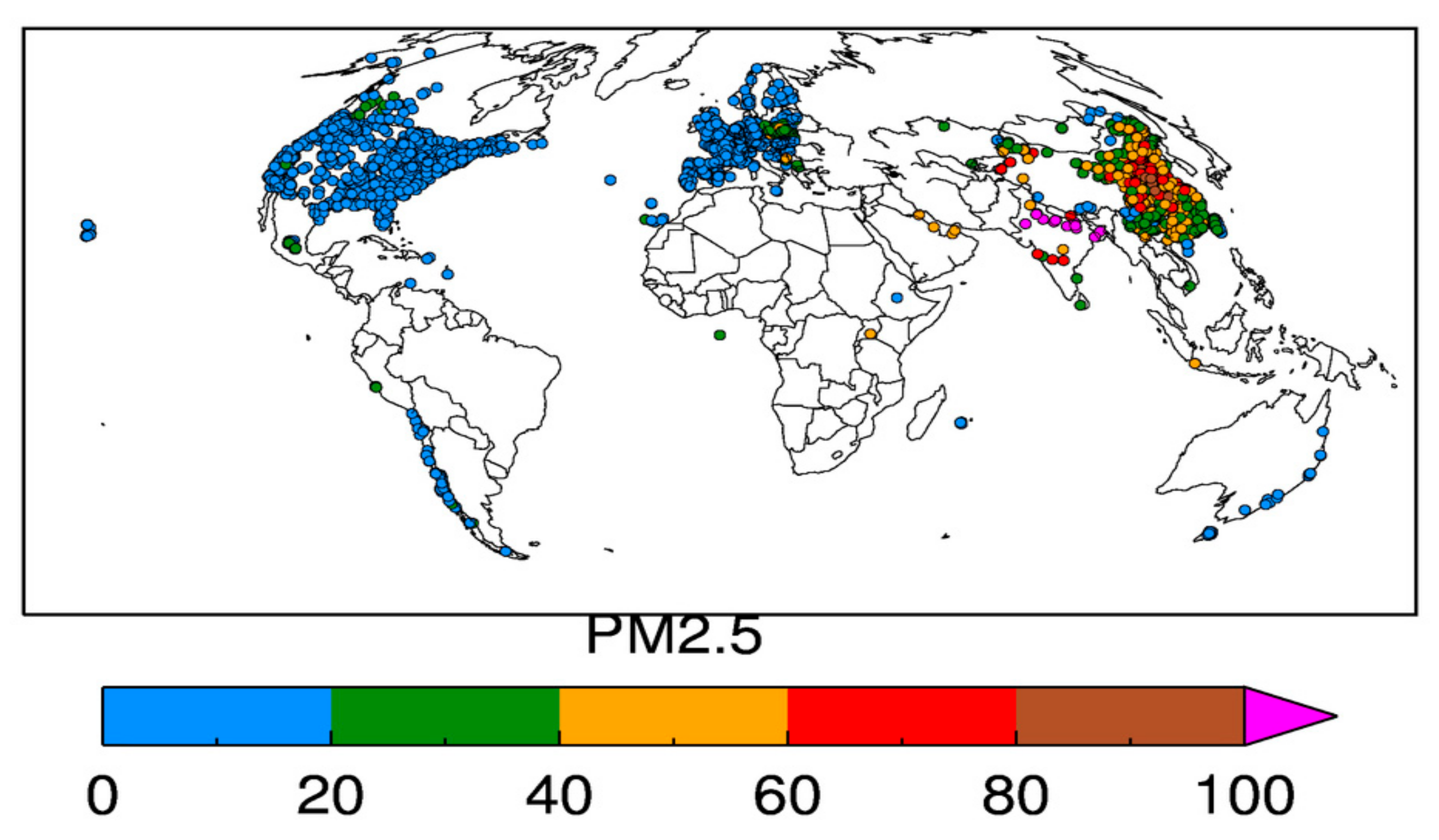
  • We first used the level 2 AOD at 0.1 × 0.1-degree spatial resolution to match with the PM2.5 data from global point locations both in space and time. For simplicity, 24-h averaged PM2.5 values are collocated with daily AOD values. The spatial collocation is performed by selecting the nearest satellite grid to the surface monitor.
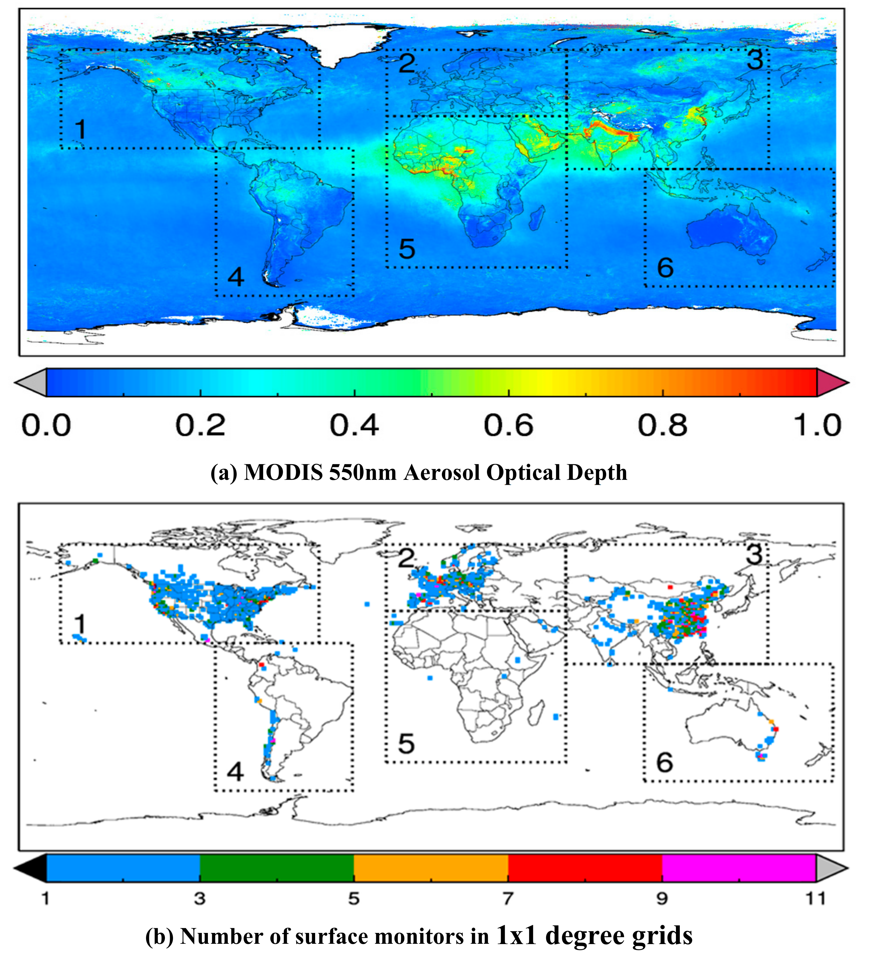
  • Then we averaged the AOD data over 3 × 3 grids centered around the nearest grid to obtain an AOD value for a given day at a given PM2.5 locations. This way, we have spatial–temporal collocated AOD–PM2.5 data sets for 3352 ground monitors.
  • We then present our results acquired at individual stations but grouped in 1 × 1 degree grids.

4. Results

Figure 1 shows the 1 × 1 degree-gridded global distribution of both the mid visible MODIS mean AOD (Figure 1a) for 2019 and the number of PM2.5 monitors available in each grid (1b). Figure 1a shows that satellite data can provide a global columnar AOD value, whereas the number of ground monitors is limited on a global basis (Figure 1b). Figure 1a also shows the typical annual average hot spots for aerosols, including biomass burning in South America and Africa, dust aerosols in the Sahara, and pollution aerosols in India and China, possibly mixed with dust & smoke. Enhanced AOD values are also shown in Western Canada and in the United States due to the large fires during summer 2019. The Southern hemisphere oceans are relatively clean, whereas the Atlantic Ocean has a noticeable dust aerosol transport pattern from the Saharan desert from the East to West Atlantic. Figure 1b shows that most of the ground monitors are in the United States, Europe, and parts of China, whereas very little ground monitoring is available in the rest of the world. Another important aspect shown in Figure 1b is the density of ground monitors with hourly measurements. In most of the world where monitors are available, the number of stations within 12,000 km2 (~1 × 1 degree) area is limited (<3) except for some large urban centers with a greater number of monitors (>7). Very few grids have greater than ten monitors and, therefore, all those grids are assigned the color gray in Figure 1b. Satellite data therefore becomes important for providing a global distribution of aerosol concentrations. Even when no ground monitors are available, the satellite AOD coupled with appropriate meteorology (Equation (1)) can provide the best estimate of surface PM2.5. Figure 1b also shows seven boxes, which are regions that we provide statistics for in Table 1. Table 1 indicates that globally there are 3352 ground monitors that are available with South America, Africa, and Australia having fewer than 100 ground monitors. Even though Asia appears to have numerous ground monitors (1508), given the population density, the number of ground monitors is still inadequate.
Figure 2 shows relevant frequency distributions for satellite AOD and surface PM2.5 for five years from collocated AOD–PM2.5 data. Figure 2a shows a tremendous increase in the number of surface monitors from 2015 to 2019, which became available in OpenAQ systems. It is important to note that after adding stations in the database, OpenAQ only obtained data in forward processing mode and does not go back and retrieve past datasets. Therefore, the change in the number of stations by year to year is solely related to when OpenAQ added those stations and does not reflect the actual data record those individual stations may have through other databases. It is important to note that unlike OpenAQ, information on individual stations record, and associated metadata are not readily available from other platforms. From 2015 to 2019, the number of ground monitors in Europe increased from 60 to 713; Asia from 12 to 1478; Australia from 1 to 27; Africa from 2 to 27; North America from 1 to 850; and South America from 44 to 78. While there is an increase in open data access of ground monitoring capability in most regions, Asia by far had the largest increase, which is encouraging given the high concentrations of aerosols in this region (Figure 1a). Figure 2b shows the number of AOD–PM2.5 pairs that are available each year for analysis. Globally, nearly a million pairs of AOD–PM2.5 data are available (Table 1), with 175,000 to 277,000 pairs available as a function of the four Northern hemisphere seasons (Table 2). This is important progress since an increase in the number of surface monitors with OpenAQ will continue to improve our ability to estimate surface PM2.5 from satellite data sets more reliably. This is especially true for statistical methods that rely on having adequate number of AOD–PM2.5 pairs for developing and implementing the algorithms. Note that even though the number of stations has increased from 2015 to 2019, the number of available AOD–PM2.5 pairs are less in 2019 because only a partial year of data was available at the time of writing this manuscript.
Figure 2c,d, show the frequency distribution of satellite AOD and surface PM2.5 for five years. The frequency distribution patterns are generally the same between the satellite and surface monitors with values skewed towards smaller AOD’s and lowered PM2.5, which is to be expected as more monitors were added over the years. It is important to note that the number of values with higher PM2.5 (and AOD) is higher for certain years (e.g., 2018) when compared to others (e.g., 2016), which could serve as important pieces of information for studies assessing short to midterm trends on air quality. Table 2 also indicates that the highest mean annual AOD and PM2.5 are in Asia with values of 0.435 and 57 μgm−3, respectively. The World Health Organization, air quality guidelines, denote annual mean PM2.5 concentrations of 35 μgm−3are associated with a 15% higher long-term mortality risk. The annual mean values in Region 4 (Asia) are about 1.5 times more than the WHO guidelines. Australia has the lowest AOD and PM2.5 with annual mean PM2.5 values below 10 μgm−3. Seasonally, the highest PM2.5 values are during the Northern hemisphere winter months of 30.6 μgm−3. These numbers are consistent with other published regional studies. There are several important factors for the varying number of AOD–PM2.5 pairs among regions/countries. One factor is the timing of data availability in the OpenAQ system for that region/country. As mentioned before, OpenAQ does not retrieve historical data sets and only provides data in forward processing mode. For example, the lower number of pairs in China and Europe demonstrate that these data became available much later in the study period. The decrease in the number of paired data from 2018 to 2019 is due to a reduction in the number of monitoring stations as we only had data for the first quarter of 2019. (Figure 2a) and other factors, including cloud cover and aerosol retrieval algorithm limitations (i.e., snow/ice on the surface, false aerosol detection) [36]. Since these are optical measurements from polar-orbiting satellites, cloud cover is indeed a limiting factor for calculating surface PM2.5 from satellites. While it is to be expected that daily measurements are hampered due to cloud cover, a focused study that assessed the cloud cover issue over the United States, showed that mean differences between PM2.5 reported by ground monitors and PM2.5 calculated from ground monitors during the satellite overpass times during cloud-free conditions are less than ± 2.5μgm−3, although this value varies by season and location [36]. This study further concluded that cloud cover is not a major problem for inferring monthly to yearly PM2.5 from space-borne sensors. The use of geostationary satellite data can alleviate some of the issues surrounding cloud cover for studies that require a daily estimate of PM2.5 from satellites, in locations where there are no ground monitors. For studies that require monthly to seasonal and annual averages repeated sampling from satellites offers an effective solution for estimating PM2.5.
Figure 3 shows the 1 × 1-degree spatial distribution of the linear correlation coefficient between PM2.5 and AOD (Figure 3a), slope of the relationship (Figure 3b), the number of pairs in a 1 × 1-degree box (Figure 3c), and the intercept (Figure 3d). The correlation coefficient R varies across the regions (Table 1) with values ranging from 0.1 (South America) to 0.6 (North America, and Africa) and seasonally (Table 2) the northern hemisphere winter months have the highest correlation of 0.65. If aerosols are well mixed and primarily in the boundary layer, then column AOD is representative of the surface pollution that increases the correlation coefficient. Based on Equation (1), it can be seen that although there is a geophysical relationship between surface PM2.5 and column AOD, many variables are needed to estimate PM2.5 from satellite data. Correlations are generally lower in Europe even though the number of ground monitors and the number of paired AOD–PM2.5 are high, which could be due to many reasons and analysis of this issue is beyond the scope of this paper.
Figure 4 shows the frequency distribution of 1 × 1 degree grids of (a) the number of surface monitors, (b) 1 × 1-degree correlation coefficient, (c) slope, and (d) intercept of the AOD–PM2.5 relationships. In an ideal scenario, the number of ground monitors in each 1 × 1 grid will be uniform. As an example, Figure 4a shows that about four hundred 1 × 1 degree grids have at least one surface monitor, whereas less than 20 grids have 10 surface monitors or more. This is the reason for choosing the color scale that is seen in Figure 1b. Comparing this to the spatial distribution in Figure 1b, it can be seen that the distribution of ground monitors even in densely populated areas is uneven. Figure 4b shows the linear correlation coefficient between AOD and PM2.5 for 1 × 1 degree grids. While the majority of the R values are positive, there are a few negative correlations. The frequency distribution indicates that correlation has a peak frequency of approximately 0.2, with a large spread in values. Table 1 indicates that if we were to remove the correlations from Europe (R = 0.12, and N = 775) and South America (R = 0.10, N = 90), the global annual correlation coefficients would be much higher. This indicates that closer scrutiny of the AOD–PM2.5 relationships need to be conducted over regions with low correlation coefficients to determine which of the variables in Equation (1) is causing the differences. Figure 4c shows the slope values of AOD–PM2.5 relationships. The global mean slope value averaged over all AOD–PM2.5 pairs and seasons is 54 µgm−3 for a unit AOD, and seasonally, it varies from 22 μgm−3 (summer) to 81.8 μgm−3 (winter). The corresponding mean PM2.5 values averaged over all ground monitors is higher than all other seasons with a value of 30.6 μgm−3. Figure 4d shows a large spread in intercept values as well and the global mean intercept is 8.6 μgm−3. The range of slopes and intercepts reported here are in line with prior research [2], and the spread in values is indicative of the heterogeneity of aerosol type, vertical distribution, and the associated meteorology. It is especially challenging in areas where there is more than one type of predominant aerosol with high spatial and vertical variability. For example, in East Asia during Northern Hemisphere Spring seasons, desert dust could be mixed with pollutions aerosols around urban centers that creates numerous challenges for retrieving AOD and estimating PM2.5.

5. Discussion and Conclusions

In 2003, Wang and Christopher reported that MODIS satellite data and products have a high potential for estimating surface PM2.5 concentrations. Since then, research studies that utilize various satellite data and products to estimate surface PM2.5 concentrations have grown exponentially. However, a majority of studies require the use of ground monitors to ‘calibrate’ the satellite aerosol optical depth. Even studies that do not follow that approach require ground monitors to validate the results derived from satellite data. In this study, we have used 5 years of MODIS mid visible AOD in conjunction with globally available PM2.5 data from ground monitors to discuss the spatial and temporal distribution of the AOD–PM2.5 relationships along with other relevant statistics. Our results indicate that currently, more than 3000 ground monitors are now available for PM2.5 research. While two decades of high-quality satellite data are available, there has been an increase in ground monitors only over the last five years. Globally, averaged over all seasons, for a unit AOD, the PM2.5 is 54 μgm−3 with an intercept of 8.6 μgm−3 although this relationship varies spatially and temporally. The global annual mean correlation coefficient is 0.55, and some regions have higher values (e.g., North America) when compared to others (e.g., Europe). The use of satellite data for PM2.5 is indeed promising with various new satellites [18] to be launched in the near future that will provide valuable information on air quality.

Author Contributions

S.C. led the writing of the article and P.G. was responsible for generating the figures. Both authors played an equal role in editing, revising and reviewing the manuscript. All authors have read and agree to the published version of the manuscript.

Funding

Pawan Gupta was partially supported by the NASA ROSES program NNH17ZDA001N-TASNPP: The Science of Terra, Aqua, and Suomi NPP Abstracts of Selected Proposals and Sundar A Christopher was supported by the Earth System Science Center.

Acknowledgments

We thank the OpenAQ team and community for acquiring and making global data available for the research. We also thank OpenAQ Director, Christa Hasenkopf who helped with PM2.5 datasets. We thank MCST for their efforts to maintain and improve the radiometric quality of MODIS data, and LAADS/MODAPS for the continued processing of the MODIS products.

Conflicts of Interest

The authors declare no conflict of interest. The funders had no role in the design of the study; in the collection, analyses, or interpretation of data; in the writing of the manuscript, or in the decision to publish the results.

Appendix A

A global distribution of PM2.5 at the surface monitoring sites provides an important perspective for air quality studies. Although the WHO provides an annual average of 10 μgm−3 as a guideline that all countries should achieve, there is still much work to be done in getting to those estimates. Figure A1 provides the annual mean values, showing that most of the Eastern hemisphere has annual PM2.5 values nearly four times higher than the 10 μgm−3 guideline. This is a serious problem because areas where the PM2.5 is high is where the population density is high. Figure A1 also highlights the need for more surface monitors to assess PM2.5. Even though satellite data provide a powerful mechanism to estimate PM2.5 where surface monitors are not available, having surface monitors will allow us to further reduce uncertainties in these estimates.
Figure A1. Global distribution of annual mean PM2.5 concentrations in μgm−3 from ground monitors for 2018. Note that there is reasonable coverage in North America, Europe, and parts of China; much of the world has no monitors to assess PM2.5 concentrations.
Remotesensing 12 01985 g0a1

References

  1. Ramaswamy, V.; Collins, W.; Haywood, J.; Lean, J.; Mahowald, N.; Myhre, G.; Naik, V.; Shine, K.P.; Soden, B.; Stenchikov, G.; et al. Radiative Forcing of Climate: The Historical Evolution of the Radiative Forcing Concept, the Forcing Agents and their Quantification, and Applications. Meteorol. Monogr. 2018, 59, 14.1–14.101. [Google Scholar] [CrossRef]
  2. Hoff, R.M.; Christopher, S.A.; Hidy, G.; Sharma, P.; Poulsen, T.; Kalluri, P.; Hoff, S.; Bundy, D.; Nelson, M.; Zelle, B.; et al. Remote Sensing of Particulate Pollution from Space: Have We Reached the Promised Land? J. Air Waste Manag. Assoc. 2009, 59, 645–675. [Google Scholar] [CrossRef] [PubMed]
  3. Bell, J.N.; Power, S.A.; Jarraud, N.; Agrawal, M.; Davies, C. The effects of air pollution on urban ecosystems and agriculture. Int. J. Sustain. Dev. World Ecol. 2011, 18, 226–235. [Google Scholar] [CrossRef]
  4. Cohen, A.; Brauer, M.; Burnett, R.; Anderson, H.R.; Frostad, J.; Estep, K.; Balakrishnan, K.; Brunekreef, B.; Dandona, L.; Dandona, R.; et al. Estimates and 25-year trends of the global burden of disease attributable to ambient air pollution: an analysis of data from the Global Burden of Diseases Study 2015. Lancet 2017, 389, 1907–1918. [Google Scholar] [CrossRef] [Green Version]
  5. Burnett, R. Global Estiamtes of mortality associaed with long erm exposure to outdoor fine particulate matter. Proc. Natl. Acad. Sci. USA 2018, 115, 9592–9597. [Google Scholar] [CrossRef] [Green Version]
  6. World Health Organisation (WHO). Ambient Air Pollution: A Global Assessment of Exposure and Burden of Disease; RePEc: Geneva, Switzerland, 2016. [Google Scholar]
  7. West, J.J.; Cohen, A.; Dentener, F.; Brunekreef, B.; Zhu, T.; Armstrong, B.; Bell, M.; Brauer, M.; Carmichael, G.R.; Costa, D.L.; et al. What We Breathe Impacts Our Health: Improving Understanding of the Link between Air Pollution and Health. Environ. Sci. Technol. 2016, 50, 4895–4904. [Google Scholar] [CrossRef]
  8. Balluz, L.; Wen, X.-J.; Town, M.; Shire, J.D.; Qualter, J.; Mokdad, A. Ischemic Heart Disease and Ambient Air Pollution of Particulate Matter 2.5 in 51 Counties in the U.S. Public Health Rep. 2007, 122, 626–633. [Google Scholar] [CrossRef]
  9. Allen, G.; Sioutas, C.; Koutrakis, P.; Reiss, R.; Lurmann, F.W.; Roberts, P.T. Evaluation of the TEOM method for measurement of ambient particulate mass in urban areas. J. Air Waste Manag. Assoc. 1997, 47, 682–689. [Google Scholar] [CrossRef]
  10. Feenstra, B.; Papapostolou, V.; Hasheminassab, S.; Zhang, H.; Der Boghossian, B.; Cocker, D.; Polidori, A. Performance evaluation of twelve low-cost PM2.5 sensors at an ambient air monitoring site. Atmos. Environ. 2019, 216, 116946. [Google Scholar] [CrossRef]
  11. Levy, R.C.; Mattoo, S.; Munchak, L.A.; Remer, L.A.; Sayer, A.M.; Patadia, F.; Hsu, N.C. The Collection 6 MODIS aerosol products over land and ocean. Atmos. Meas. Tech. 2013, 6, 2989–3034. [Google Scholar] [CrossRef] [Green Version]
  12. Chudnovsky, A.A.; Kostinski, A.; Lyapustin, A.; Koutrakis, P. Spatial scales of pollution from variable resolution satellite imaging. Environ. Pollut. 2013, 172, 131–138. [Google Scholar] [CrossRef] [PubMed]
  13. Chudnovsky, A.; Tang, C.; Lyapustin, A.; Wang, Y.; Schwartz, J.; Koutrakis, P. A critical assessment of high resolution aerosol optical depth (AOD) retrievals for fine particulate matter (PM) predictions. Atmos. Chem. Phys. Discuss. 2013, 13, 14581–14611. [Google Scholar] [CrossRef] [Green Version]
  14. Mei, L.; Strandgren, J.; Rozanov, V.; Vountas, M.; Burrows, J.P.; Wang, Y. A study of the impact of spatial resolution on the estimation of particle matter concentration from the aerosol optical depth retrieved from satellite observations. Int. J. Remote. Sens. 2019, 40, 7084–7112. [Google Scholar] [CrossRef]
  15. Wang, J. Intercomparison between satellite-derived aerosol optical thickness and PM2.5mass: Implications for air quality studies. Geophys. Res. Lett. 2003, 30. [Google Scholar] [CrossRef]
  16. Liu, Y.; Paciorek, C.; Koutrakis, P. Estimating Regional Spatial and Temporal Variability of PM2.5 Concentrations Using Satellite Data, Meteorology, and Land Use Information. Environ. Health Perspect. 2009, 117, 886–892. [Google Scholar] [CrossRef] [Green Version]
  17. Van Donkelaar, A.; Martin, R.V.; Li, C.; Burnett, R.T. Regional Estimates of Chemical Composition of Fine Particulate Matter Using a Combined Geoscience-Statistical Method with Information from Satellites, Models, and Monitors. Environ. Sci. Technol. 2019, 53, 2595–2611. [Google Scholar] [CrossRef] [Green Version]
  18. Liu, Y.; Diner, D.J. Multi-Angle Imager for Aerosols: A Satellite Investigation to Benefit Public Health. Public Health Rep. 2017, 132, 14–17. [Google Scholar] [CrossRef]
  19. Koelemeijer, R.; Homan, C.; Matthijsen, J. Comparison of spatial and temporal variations of aerosol optical thickness and particulate matter over Europe. Atmos. Environ. 2006, 40, 5304–5315. [Google Scholar] [CrossRef]
  20. Chu, Y.; Liu, Y.; Li, X.; Liu, Z.; Lu, H.; Lu, Y.; Mao, Z.; Chen, X.; Li, N.; Ren, M.; et al. A Review on Predicting Ground PM2.5 Concentration Using Satellite Aerosol Optical Depth. Atmosphere 2016, 7, 129. [Google Scholar] [CrossRef] [Green Version]
  21. Gupta, P.; Christopher, S.A. Particulate matter air quality assessment using integrated surface, satellite, and meteorological products: Multiple regression approach. J. Geophys. Res. Space Phys. 2009, 114. [Google Scholar] [CrossRef] [Green Version]
  22. Liu, Y.; Park, R.J.; Jacob, D.J.; Li, Q.; Kilaru, V.; A Sarnat, J. Mapping annual mean ground-level PM2.5concentrations using Multiangle Imaging Spectroradiometer aerosol optical thickness over the contiguous United States. J. Geophys. Res. Space Phys. 2004, 109. [Google Scholar] [CrossRef]
  23. Lee, H.J.; Liu, Y.; Coull, B.A.; Schwartz, J.; Koutrakis, P. A novel calibration approach of MODIS AOD data to predict PM2.5 concentrations. Atmos. Chem. Phys. 2011, 11, 7991–8002. [Google Scholar] [CrossRef] [Green Version]
  24. Kloog, I.; Nordio, F.; Coull, B.A.; Schwartz, J. Incorporating Local Land Use Regression And Satellite Aerosol Optical Depth In A Hybrid Model Of Spatiotemporal PM2.5Exposures In The Mid-Atlantic States. Environ. Sci. Technol. 2012, 46, 11913–11921. [Google Scholar] [CrossRef] [PubMed] [Green Version]
  25. Beckerman, B.S.; Jerrett, M.; Serre, M.L.; Martin, R.V.; Lee, S.-J.; Van Donkelaar, A.; Ross, Z.; Su, J.; Burnett, R.T. A Hybrid Approach to Estimating National Scale Spatiotemporal Variability of PM2.5in the Contiguous United States. Environ. Sci. Technol. 2013, 47, 7233–7241. [Google Scholar] [CrossRef] [PubMed] [Green Version]
  26. Hu, X.; Waller, L.A.; Al-Hamdan, M.Z.; Crosson, W.L.; Mauric, G.E., Jr.; Estes, S.M.; Quattrochi, D.A.; Sarnat, J.A.; Liu, Y. Estimating ground-level PM2.5 concentrations in the southeastern U.S. using geographically weighted regression. Environ. Res. 2013, 121, 1–10. [Google Scholar] [CrossRef]
  27. Song, W.; Jia, H.; Huang, J.; Zhang, Y. A satellite-based geographically weighted regression model for regional PM2.5 estimation over the Pearl River Delta region in China. Remote. Sens. Environ. 2014, 154, 1–7. [Google Scholar] [CrossRef]
  28. Gupta, P.; Christopher, S.A. Particulate matter air quality assessment using integrated surface, satellite, and meteorological products: 2. A neural network approach. J. Geophys. Res. Space Phys. 2009, 114. [Google Scholar] [CrossRef]
  29. Karimian, H.; Li, Q.; Wu, C.; Qi, Y.; Mo, Y.; Chen, G.; Zhang, X.; Sachdeva, S.; Kaimian, H. Evaluation of Different Machine Learning Approaches to Forecasting PM2.5 Mass Concentrations. Aerosol Air Qual. Res. 2019, 19, 1400–1410. [Google Scholar] [CrossRef] [Green Version]
  30. Hu, X.; Belle, J.; Meng, X.; Wildani, A.; Waller, L.A.; Strickland, M.J.; Liu, Y.; Kelly, J.T.; Jang, C.J.; Timin, B.; et al. Estimating PM2.5Concentrations in the Conterminous United States Using the Random Forest Approach. Environ. Sci. Technol. 2017, 51, 6936–6944. [Google Scholar] [CrossRef]
  31. Pak, U.; Ma, J.; Ryu, U.; Ryom, K.; Juhyok, U.; Pak, K.; Pak, C. Deep learning-based PM2.5 prediction considering the spatiotemporal correlations: A case study of Beijing, China. Sci. Total. Environ. 2019, 699, 133561. [Google Scholar] [CrossRef]
  32. Gupta, P.; Levy, R.; Remer, L.; Patadia, F.; Christopher, S.A. High Resolution Gridded Level 3 Aerosol Optical Depth Data from MODIS, to be submitted to Geoscience Data Journal, 2020, to be submitted.
  33. Remer, L.A.; Mattoo, S.; Levy, R.C.; Munchak, L.A. MODIS 3 km aerosol product: algorithm and global perspective. Atmos. Meas. Tech. 2013, 6, 1829–1844. [Google Scholar] [CrossRef] [Green Version]
  34. Gupta, P.; Remer, L.A.; Levy, R.C.; Mattoo, S. Validation of MODIS 3 km land aerosol optical depth from NASA’s EOS Terra and Aqua missions. Atmos. Meas. Tech. 2018, 11, 3145–3159. [Google Scholar] [CrossRef] [Green Version]
  35. Wei, J.; Li, Z.; Peng, Y.; Sun, L. MODIS Collection 6.1 aerosol optical depth products over land and ocean: validation and comparison. Atmos. Environ. 2019, 201, 428–440. [Google Scholar] [CrossRef]
  36. Christopher, S.; Gupta, P. Satellite remote sensing of particulate matter air quality: the cloud-cover problem. J. Air Waste Manag. Assoc. 2010, 60, 596–602. [Google Scholar] [CrossRef]
Figure 1. (a) Global distribution of aerosol optical depth (AOD) from combined Terra and Aqua Moderate Resolution Imaging Spectroradiometer (MODIS) for 2019 and (b) number of surface particulate matter with aerodynamic diameters less than 2.5 µm (PM2.5) monitors grouped within each 1 × 1 degree box for 2019. Relevant statistics for the rectangular boxes are shown in Table 1.
Remotesensing 12 01985 g001
Figure 2. Frequency distribution for five years of (a) number of ground monitors by year, (b) number of collocated pairs by year, (c) satellite AOD in the collocated data, and (d) surface PM2.5 in the collocated data sets.
Remotesensing 12 01985 g002
Figure 3. Global distribution of AOD–PM2.5 relationship statistics in 1 × 1 degree grids, (a) Linear Correlation Coefficient, (b) Slope, (c) Number of surface Monitors, and (d) Intercept.
Remotesensing 12 01985 g003
Figure 4. The frequency distribution of the AOD–PM2.5 relationships. in 1 × 1 degree grids for (a) number of surface monitors/stations, (b) linear correlation coefficient (R), (c) slope (m), (d) and intercept (c).
Remotesensing 12 01985 g004
Table 1. Regional and global statistics of AOD–PM2.5 pairs where R, m, and c are linear correlation coefficient, slope, and intercept, respectively. The regions are outlined and numbered as various rectangular boxes in Figure 1.
Region NumberRegionNumber of StationsNumber of PairsRmcMean AODMean PM2.5
1North America 1056507,0920.5524.46.00.1499.6
2Europe 775188,7690.128.912.60.15313.9
3Asia 1508159,4400.4955.033.00.43557.0
4South America 9049,1630.1019.417.80.10019.8
5Africa 3057280.5665.47.90.26525.0
6Australia 6115,2370.5545.23.90.0918.0
Global3352925,8170.5554.18.60.1919.3
Table 2. Seasonal Distribution of AOD–PM2.5 statistics for the globe where R, m, and c are linear correlation coefficient, Slope, and Intercept respectively.
SeasonNumbers of StationsNumbers of PairsRmcMean AODMean PM2.5
DJF3321175,3870.6581.814.10.2030.6
MAM3432230,4430.6262.05.50.1917.6
JJA2127242,4770.4622.5 7.30.2212.2
SON3469277,5100.5958.99.30.1819.7

