Article

Appraisal of SMAP Operational Soil Moisture Product from a Global Perspective

by
Swati Suman
1,
Prashant K. Srivastava
1,2,*,
George P. Petropoulos
3,
Dharmendra K. Pandey
4 and
Peggy E. O’Neill
5
1
Remote Sensing Laboratory, Institute of Environment and Sustainable Development, Banaras Hindu University, Varanasi 221005, India
2
DST-Mahamana Centre for Excellence in Climate Change Research, Institute of Environment and Sustainable Development, Banaras Hindu University, Varanasi 221005, India
3
Department of Geography, Harokopio University of Athens, El. Venizelou 70, Kallithea, 17671 Athens, Greece
4
Space Applications Centre, Indian Space Research Organization, Ahmedabad 380015, India
5
Hydrological Sciences Laboratory, NASA Goddard Space Flight Centre, Greenbelt, MD 20771, USA
*
Author to whom correspondence should be addressed.
Remote Sens. 2020, 12(12), 1977; https://doi.org/10.3390/rs12121977
Submission received: 7 May 2020 / Revised: 12 June 2020 / Accepted: 15 June 2020 / Published: 19 June 2020

Abstract

:
Space-borne soil moisture (SM) satellite products such as those available from Soil Moisture Active Passive (SMAP) offer unique opportunities for global and frequent monitoring of SM and also to understand its spatiotemporal variability. The present study investigates the performance of the SMAP L4 SM product at selected experimental sites across four continents, namely North America, Europe, Asia and Australia. This product provides global scale SM estimates at 9 km × 9 km spatial resolution at daily intervals. For the product evaluation, co-orbital in situ SM measurements were used, acquired at 14 test sites in North America, Europe, and Australia belonging to the International Soil Moisture Network (ISMN) and local networks in India. The satellite SM estimates of up to 0–5 cm soil layer were compared against collocated ground measurements using a series of statistical scores. Overall, the best performance of the SMAP product was found in North America (RMSE = 0.05 m3/m3) followed by Australia (RMSE = 0.08 m3/m3), Asia (RMSE = 0.09 m3/m3) and Europe (RMSE = 0.14 m3/m3). Our findings provide important insights into the spatiotemporal variability of the specific operational SM product in different ecosystems and environments. This study also furnishes an independent verification of this global product, which is of international interest given its suitability for a wide range of practical and research applications.

Graphical Abstract

1. Introduction

Soil moisture (SM) is a very important environmental parameter having a key role in a number of physical processes of the Earth’s system, affecting the climate directly or indirectly [1,2,3]. Information on its spatiotemporal variability is crucial in the Earth’s climate system as it is the key parameter regulating energy and mass exchanges at the earth-atmosphere interface [4,5]. The large spatial and temporal variability of SM is regarded as one of the main parameters required in understanding the role of SM in hydrology, ecosystems and biogeochemical cycles [6,7]. Accurate information on its spatiotemporal variability can inform sustainable water resources management, the study of ecosystems and ecological processes [8,9,10], plant water requirements and plant growth and productivity (e.g., [11,12]).
Despite its high importance, it is hard-to-measure parameter on a routine basis over large areas using traditional ground instrumentation due to the large spatial and temporal variability it exhibits [13]. Earth observation satellites (EOS) provide the best alternative to ground observations in deriving SM over large regions and different geographical scales. Over the last three decades, advances in EOS have allowed the development of a range of techniques that have shown promise in predicting near-surface SM [14,15]. Several approaches have been developed using EOS data acquired in the visible/infrared parts of the electromagnetic radiation spectrum (EMR), which are, however, limited by the low penetration power of optical radiation and cloud cover. On the other hand, the use of microwave (MW) EOS data overcomes this issue due to their all-weather, day and night data acquisition capability [16,17]. A number of MW satellites, both active and passive, have been launched providing suitable data for global SM mapping. Some of the most significant of those satellite missions include the Advanced Scatterometer (ASCAT) [18], the Advanced Microwave Scanning Radiometer-Earth Observing System (AMSR-E) [19], the Advanced Microwave Scanning Radiometer 2 (AMSR2) [20], the Soil Moisture and Ocean Salinity (SMOS) mission [21], and the Soil Moisture Active Passive (SMAP) [22]. An overview of operational products available from these EOS sensors is made available by Srivastava et al. [23,24]. SM products provided by those satellites have helped to increase the accuracy of global and regional climate models for more precise and near time climate and weather forecasting. Those products have also significantly contributed towards better water resource management, irrigation scheduling, defense and emergency preparedness in case of hydrological disasters, such as floods and droughts [25,26,27,28].
Given the importance and demand globally for accurate information on the spatiotemporal variability of SM, the quality assessment of those satellite-derived SM products at a global scale is an urgent task requiring attention [29,30]. Results from such studies can help to understand the product accuracy and also to identify limitations in the retrieval algorithm that may be addressed in the future, which all together can help to improve the practical use of those products much more widely globally, in a number of research investigations and practical applications alike. Furthermore, the relationship of SM with various environmental, topographical, and technical factors makes monitoring the SM variation on a large satellite footprint an interesting matter to investigate, particularly so for the available operational products [31,32].
As such, in situ SM measurements play a crucial role in calibration and validation of satellite-based products or algorithms despite their inherent limitations. In situ SM data sets are the mainstay for calibrating and validating land surface models and the quality of SM products retrieved from space-borne microwave sensors. In addition, a long-term time series of in situ SM measurements, can themselves reveal trends in the water cycle related to climate or land cover change at local and regional scales [33]. This information can be used to develop efficient water resource management strategies. Although several local and regional meteorological and hydrological networks routinely measure SM at some locations, globally the number of long-term ground-based monitoring networks are still small and largely restricted to the mid altitude and developed world, mainly due to lack of establishment and maintenance funds [34].
In this context, an investigation of the SMAP L4 SM operational product in particular would be of key importance. To our knowledge, studies on the product SM retrieval accuracy so far are rather scarce, especially on a global scale. Such studies, if available would be studying the temporal variation and behavior of SMAP that provide key insights into the spatiotemporal variability of the specific operational SM product in different ecosystems and environments. Results would also provide significant aid in understanding the satellite SM product utility in hydrological modelling, crop modelling, precision agriculture, irrigation scheduling, crop insurance and in water resources management.
In the purview of the above, this study delivers a systematic evaluation of the SMAP L4 SM product quality implemented using collocated in situ SM measurements acquired for a period one year, from June, 2017 to July, 2018, selected due to the availability of continuous ground-based data set from several ground observational networks located on the four different continents. As part of this verification, the SM product performance in capturing the variation in the surface SM under varying land cover and seasonality were also examined, discussing also the limitations of the point-based ground SM measurements, which formed our reference data set in performing this study.

2. Materials and Methods

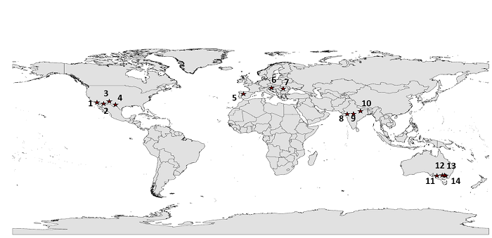
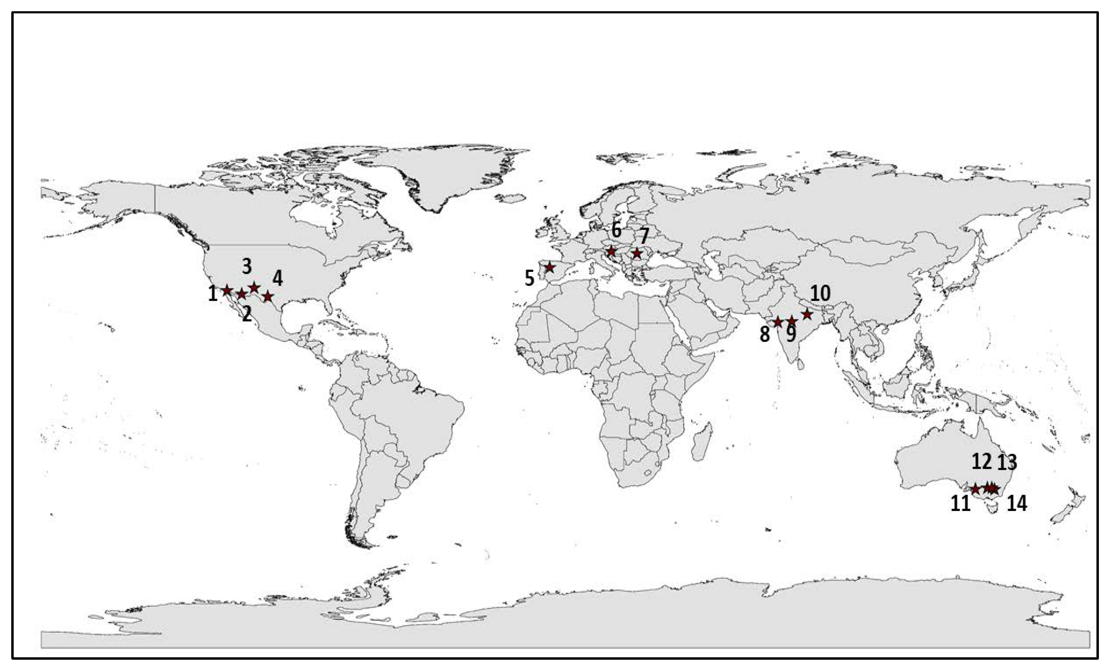
2.1. In Situ Measurements

A total of 14 sites from four different continents were selected to perform the SMAP L4 SM product validation, 4 of which located in the United States of America (USA), 3 in Europe, 3 in India and 4 in Australia. Ground measurements acquired from those sites, which formed our reference data, were acquired from different operational networks operating worldwide. Those networks included the International Soil Moisture Network (ISMN) [35], the United Nations Climate Reference Network (USCRN) [36], Romanian Soil Moisture Network (RSMN) [37], REMEDHUS [38], WEGENERNET [39], local networks on the Indian sub-continent and OZNET [40].
All 4 sites from North America were selected across the USCRN network which consists of 114 stations spread over 48 states of the USA. Each of these stations has been designed and developed strategically to be located away from the urban and suburban surroundings to avoid any locally induced biases in the climate records. The Fallbrook site is located near Santa Margarita Ecological Reserve, California. This site has a Mediterranean type of climate with hot, dry summers and mild rainy winters. The Socorro station is positioned near the Sevilleta National Wildlife Refuge Station, Minnesota and has a continental type of climate with cold and freezing winters and hot, humid summers. The Panther Junction experimental site is located in an open area of Chihuahuan desert landscape, near Lone Mountains at Big Bend National Park, Texas with a very subtropical, humid type of climate. The Arizona site is located near the Arizona-Sonora Desert Museum, Tucson and has a dry climate for most of the year.
From Europe, 3 validation sites were selected; Dumbraveni site from the Romanian Soil Moisture Network (RSMN), Feldbach from the WEGENERNET network and El Coto from REMEDHUS soil moisture network. Dumbraveni is situated in the north of the Sibiu county of Romania on the banks of the river Tarmava Mare. The site has a humid continental type of climate with cold winters and hot summers. The second site, the WEGNERNET network is located in the Alpine foreland of southeast Austria in the region of Feldbach. The Alpine foreland is at the interface between the Mediterranean and Alpine climates, having a significant amount of rainfall throughout the year. Summers here are hot with significant precipitation dominated by heavy rainfall from thunderstorms while the winters are cold with strong storms. The REMEDHUS soil moisture network is located in the central part of the Duero basin, spread across the agricultural fields in Spain. The region is mainly covered by cereal fields, vineyards and patchy areas of forests and pastures.
Furthermore, 3 experimental sites from Asia were selected located in India: the Varanasi district from Uttar Pradesh, the Hoshangabad district from Madhya Pradesh and the Anand district from Gujarat. Varanasi has a humid, subtropical type of climate with very hot, wet summers and fairly dry, cold winters but with the temperature rarely falling below freezing. The major soil types are sandy loam and clay loam and crops produced in the area are rice, pearl millet, pigeon peas, maize and horticultural crops in Kharif season and wheat, peas and maize etc., in Rabi season. Sugarcane is a major crop in the summer. The SM sensor at the Varanasi site is located at the agricultural farm in the Banaras Hindu University campus. Hoshangabad is located in the central part of the Narmada valley and on the northern fringe of Satpura plateau. The region has a dry climate except during the south west monsoon. Hoshangabad is famed for its very fertile, black alluvial soil commonly known as “black cotton” soil, considered highly argillaceous with high porosity and a fine clayey texture. Forests and agricultural land are the prominent land-cover features in the province. The sensor installed at Hoshangabad is located in a large agricultural field with large uniform patches of agricultural land nearby. The hydra probe station in the Hoshangabad region is installed at the Zonal Agriculture Research Station (ZARS) in the Pawarkheda province. Anand is located in the southern part of the Gujarat near the Gulf of Cambay, spread over an area of 2951 sq. km. Out of the total geographical area of the district about 70.5% is cultivable, having sandy loam and clay loam as the major soil types. Major crops grown in the area are rice, pearl, millet, tobacco during Kharif, and wheat in the Rabi season. The hydra probe weather station at the Anand study site is installed at the Regional Research Station (RSS) farm of the Anand Agricultural University Campus.
For Australia, we used the OZNET network situated in the Murrumbidgee catchment site in New South Wales for this investigation. This province is mainly an agricultural area, primarily used for barley/corn production on the western side, dry land cropping on the northern side and native pasture on the south and eastern side. The region is suitable for three types of farming; horticulture (grapes and citrus production); vegetable farming (onions, carrots, tomatoes, and melons) and broadacre farming (rice and wheat). An overview of the main characteristics of each of those networks and of the main features of the sensors functioning at these sites is presented in Table 1. To maintain the uniformity of the data sets, the sites were selected based on similar sensor type and homogeneous regions. For example, most of these experimental sites have a Steven’s hydra probe installed for the measurement of SM and soil temperature at similar ranges of soil depths, except the Dumbraveni site in Romania from the RSMN network which uses Decagon 5TM sensor to measure SM and temperature. The Steven’s hydra probe device is a rugged SM sensor which measures the dielectric spectrum of the soil based on the “dielectric impedance” taking into account the energy loss and energy storage across the area using 50 MHz radio frequency to measure both the components of complex dielectric permittivity: the real and imaginary part, SM, salinity and temperature. Based on the behavior of reflected signals, an onboard processor converts these signal responses and measures the soil dielectric’s permittivity which corresponds to the SM and bulk electrical conductivity (EC) measurements. This device has been a reliable resource for measuring SM and other parameters such as soil temperature and precipitation in recent years and extensively used in studies like these [41,42,43,44]. The sensor installed at the Dumbraveni site is also based on a similar concept and uses an electromagnetic field to measure the dielectric permittivity of the surrounding medium. The 5TM microprocessor measures the temperature by an onboard thermistor and the volumetric water content (VWC) using capacitance/frequency domain technology. Figure 1 below shows the locations of the validation sites used in this study across the globe.

2.2. Satellite Data Description

2.2.1. SMAP L4 Soil Moisture Product

SMAP is the first EOS mission developed by the National Aeronautics and Space Administration (NASA) in response to the National Research Council’s Decadal Survey, launched on 31 January 2015. SMAP is a sun-synchronous satellite and consists of simultaneously active (in the form of radar) and passive (in the form of radiometer) MW instruments at L-band frequency (1.2–1.4 GHz range). The SMAP provides a series of baseline data products which are available at no cost through NASA’s two Distributed Active Archive Centers (DAACs), the Alaska Satellite Facility for Level 1 radar product and the National Snow and Ice Data Center for all other products.
The SMAP L4 SM product in particular provides global surface and root zone SM estimates at 3-h temporal and 9 km spatial resolution [45]. The product is derived using an ensemble Kalman Filter (EnKF) merging SMAP L1C brightness temperature observations with the SM estimates from the NASA Catchment Land Surface model [46,47]. The model describes the vertical transfer of SM between the surface (in the top 5 cm of the soil column) and root zone (in the top 1 m of the soil column). The product is provided to the users in HDF5 format.
To study the daily variation in the SM in the natural ecosystems for different landscapes, climates, soil types and vegetation covers and assess the accuracy of the satellite SM product mapping of this behavior, in this study we used daily estimates of the satellite SM using the SMAP L4 product. Furthermore, these daily estimates were compared with the ground-measured SM values to check the performance of the SMAP L4 SM product.

2.2.2. NASA Global Precipitation Measurement Integrated Multi-SatellitE Retrievals for GPM (IMERG)

The Global Precipitation Measurement Integrated Multi-satellitE Retrievals for GPM (IMERG) is a unified algorithm to provide a multi-satellite precipitation product to the GPM mission [48]. The algorithm produces intercalibrated, gridded, merged and interpolated satellite products together with the MW (both active and passive) calibrated infrared (IR) satellite precipitation estimates, precipitation rain gauge estimates and potentially all other precipitation data at fine temporal and spatial scales for the NASA Tropical Rainfall Measurement Missions (TRMM) and GPM on a global scale [48,49]. The daily global rainfall data set from the GPM were downloaded from the website (https://pmm.nasa.gov/data-access/downloads/gpm). These data sets were further processed in MATLAB 2016a and ArcGIS 10.1 to get rainfall measurements over the selected validation sites to study the behavior of SM with incoming precipitation and also to the response and sensitivity of satellite SM for the natural processes.

2.3. Performance Statistics

The in situ measurements obtained from the ISMN at the SMAP overpass time were selected for assessing the quality of the SMAP SM product. For the quality assessment, point-shape files of the study sites were assigned in ArcMap 10.1 and were used to extract data from the SMAP L4 global SM data sets. Evaluation was done on a point to point comparison between the satellite and ground-based SM measurements. The accuracy of both measurements was assessed using four statistical scores: square of correlation (R2), root mean square error (RMSE), percentage bias (PBIAS) and degree of agreement (d) [50,51,52]. A detailed description of these statistical tests and mathematical equations are provided in Table 2.

3. Results

This section presents the results obtained after comparing the ground-based SM measurements acquired from the ISMN and other ground networks with the SMAP L4 SM global product over selected experimental sites across the four continents over a period of one year (June 2017–July 2018). The time frame of this analysis is influenced mostly by the availability of continuous in situ SM measurements at all the selected locations. Results are divided into two sections: first, to highlight the performance of both the data sets, presented using the scatter, and second, the temporal time series plots to minutely observe the behavior of the data sets over the observed time period.

3.1. North America

3.1.1. Performance Comparison at Different Stations

For the North American continent, we selected the sites from the USA mainly due to availability of continuous ground-based data sets within the selected time frame of this study. Table 3 presents the results of the statistical scores, selected for the comparison between the two data sets as explained in Section 2.3. The sites selected are mostly from the agricultural states of the USA; California, Texas, Minnesota and Arizona and have the hydra probe installed for the measurement of SM and other meteorological variables. The results showed good correlation between the ground and SMAP data sets for Fallbrook, California and Tucson, Arizona with R2 values 0.66 and 0.51 respectively, followed by the Panther Junction region from Texas (R2 = 0.43) and Socorro region from Minnesota state (R2 = 0.11). Other statistical scores for the Fallbrook region were reported as RMSE = 0.08, percentage bias (PBIAS) = −57.90 and degree of agreement (d) = 0.46. For the Tucson region the RMSE was 0.04, d was 0.65 and PBIAS was 120.60. The Fallbrook site has reported a negative PBIAS which means an underestimation by the SMAP data set. Similarly, for Panther Junction, RMSE = 0.03, d = 0.74 and PBIAS = 26.10 and for the Socorro, RMSE = 0.05, d = 0.55 and PBIAS = 56.80. In contrast to the first site, the rest of the study sites, Tucson, Panther Junction and Socorro region showed a positive PBIAS which indicates overestimation by the satellite data set. Figure 2a–d, represent the scatter plots between the in situ and SMAP SM measurements for Fallbrook, Tucson, Panther Junction and Socorro experimental sites, respectively. Based on the RMSE between both the data sets, the performance of SMAP SM was reported best at Panther Junction (0.03) followed by Tucson (0.04), Socorro (0.05) and Fallbrook (0.08). We also used degree of agreement (d) which represents the level of model prediction error and a value closer to 1 represents a perfect match. Results show best performance of the SMAP SM at Panther Junction (0.74), then Tucson (0.65), Socorro (0.55) and Fallbrook (0.46).

3.1.2. Temporal Consistency
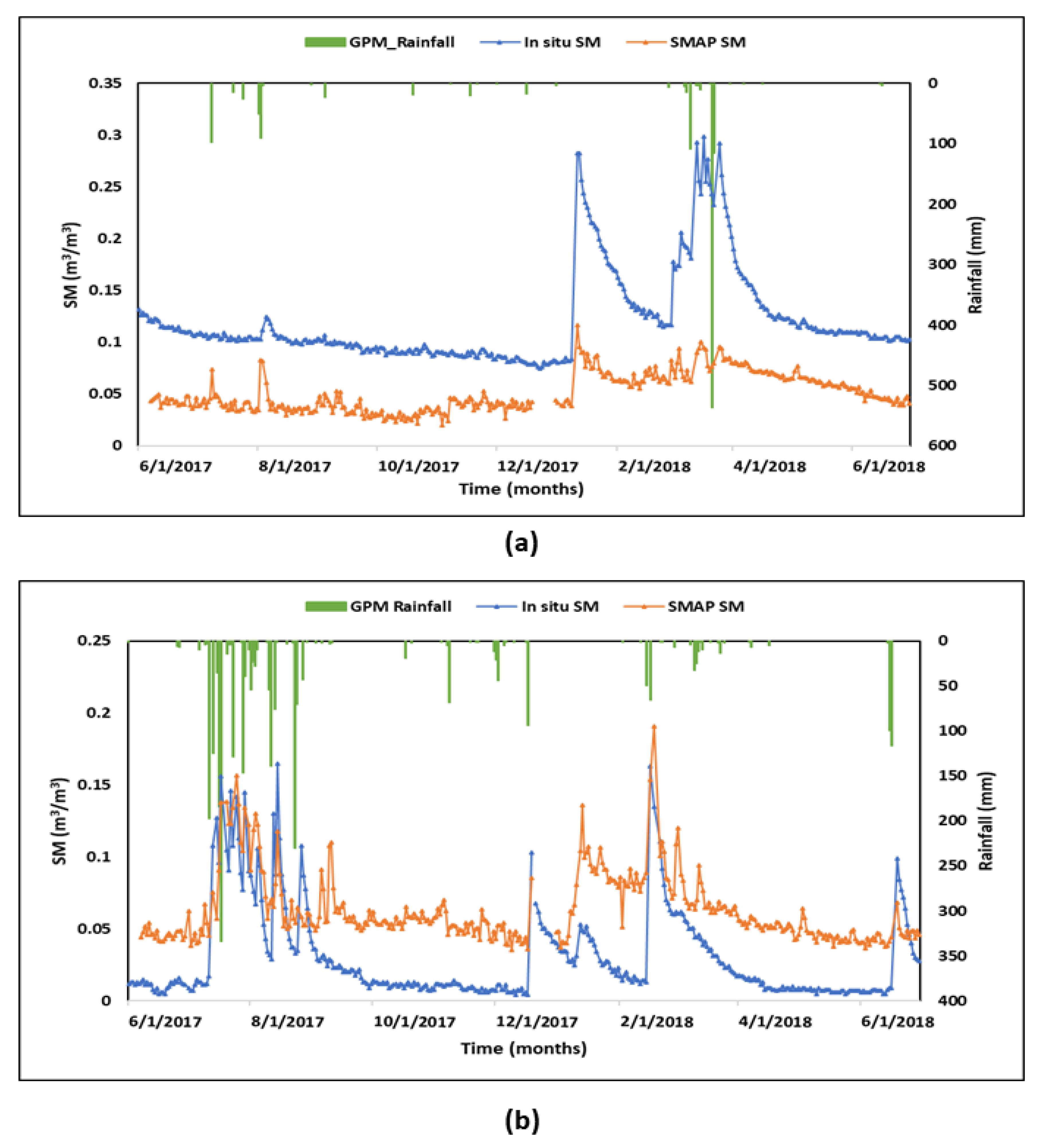
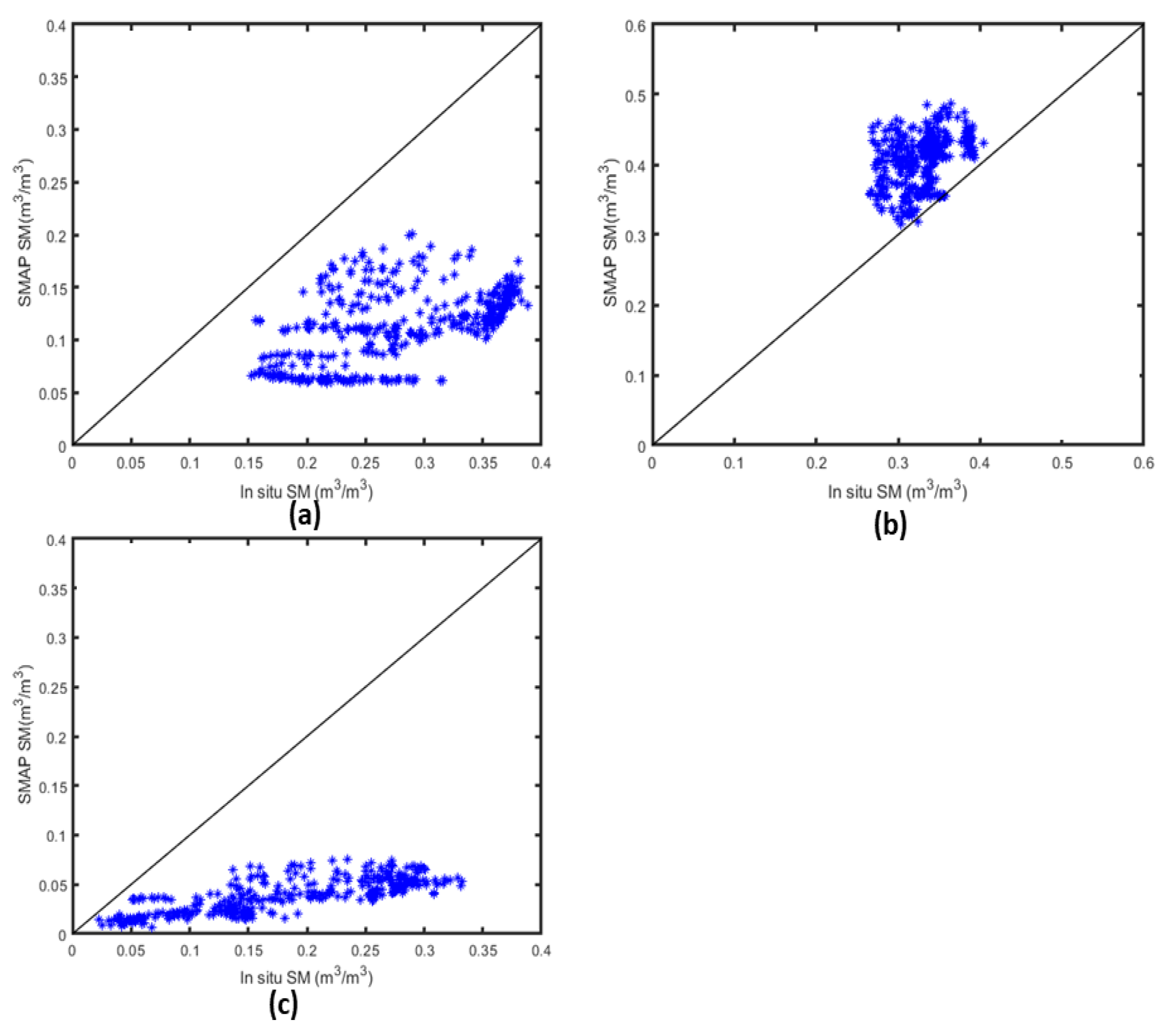
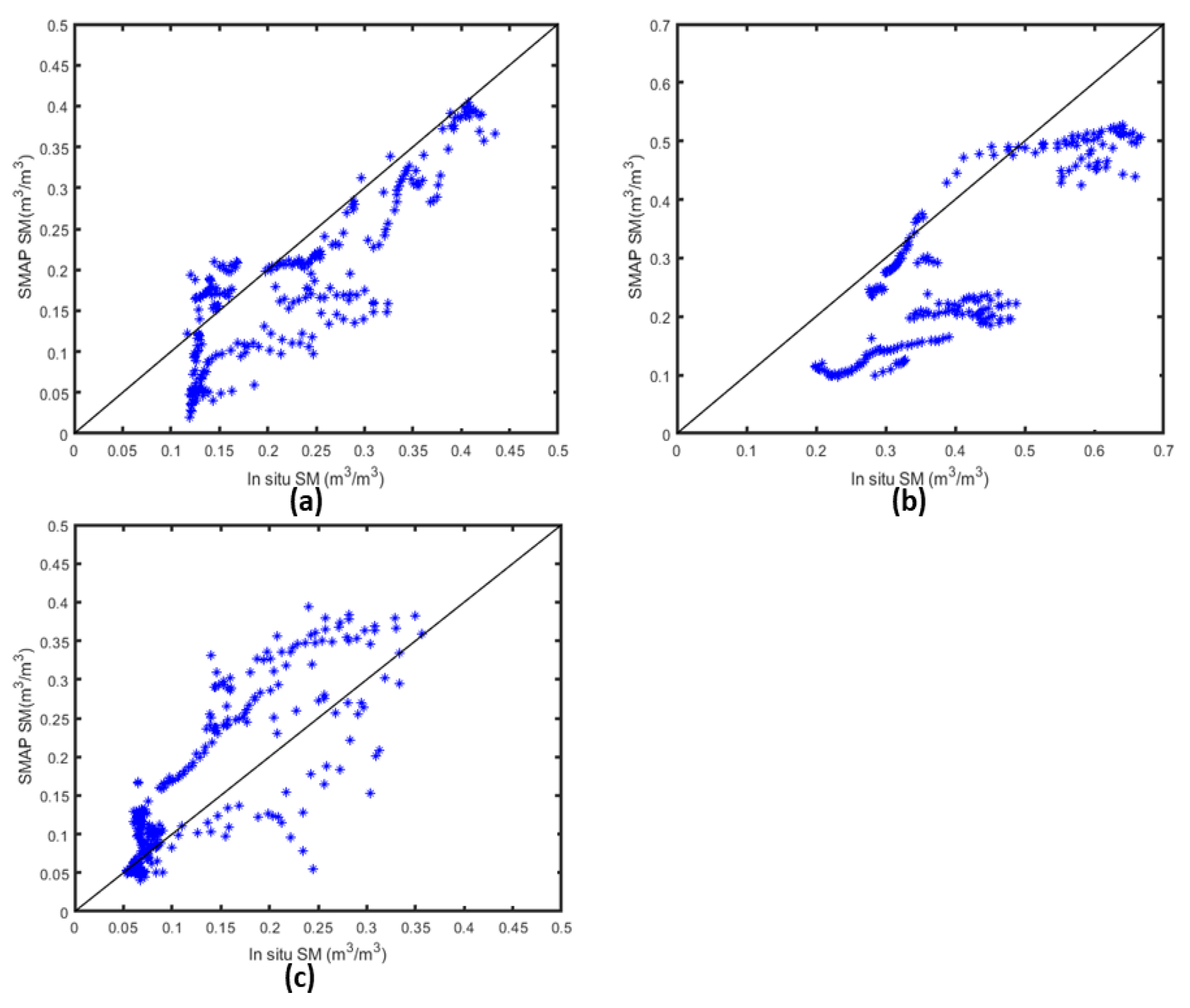
Figure 3 presents the time series plot for the in situ SM measurements and SMAP SM estimates over a period of one year (June 2017–July 2018). Figure 3a shows the variation in the selected parameters for the Fallbrook site. The PBIAS value (−57.9) indicated an underestimation of the in situ SM values by the SMAP estimates, which were clearly evident in the above figure for the entire study period, except for some days in the first week of August 2017, last week of January 2018, last week of February and first week of March, first week of May and last week of July 2018, both data sets showed similar values. The GPM rainfall data set indicates few days of rainfall during July–August 2017 and heavy downpours during March–April 2018. For the Tucson site, the overall positive PBIAS value (120.60) indicated an overestimation of SMAP SM in comparison to situ SM estimates. However, the time series plot given in the Figure 3b for Tucson, Arizona showed a mixed kind of behavior of both the data sets. Both the data sets showed close association in the early phase of the study period; during June to September 2017 and then showed a significant overestimation in mid phase specifically between October 2017 to January 2018. For a few days in the rest period of the study: during the first weeks of January, March, June and the last week of July 2018, both the data sets were comparable to in situ. Rainfall estimates showed significant amounts of rain during July–September 2017 and on a few days in December 2017 and March, April and June 2018.
Figure 4a shows the time series plot of the SMAP and in situ SM data sets over the entire study period of Panther Junction and it clearly depicts overall overestimation by the satellite data set but close association for almost the entire time period. The SMAP SM measurements when compared with the in situ data set for the entire period of this study overestimated the latter. The daily estimate of rainfall presented by the GPM rainfall data set in the plot showed heavy precipitation during June–November 2017 and on a few days during December 2017 and February, March and May 2018. During those days, both the SM data sets capture the sharp variations, indicating satisfactory performance of the data sets. For the Socorro, Minnesota, Figure 4b presents the temporal time series plots between both the data sets. For some period of time during July and August 2017, the in situ data set overestimated the SMAP estimates however, it gradually decreased. There was some data set gap between December 2017 to January 2018 and then from the last week of January to February 2018, perhaps due to some technical fault in the sensor and this resulted in data discontinuity. The rainfall estimates in the temporal graph showed significant amounts of rainfall during June–November 2017 and on a few days in the months of February, March, May and June 2018. Interestingly both the SM data sets also showed maximum fluctuation during these days of rainfall showing high sensitivity of both measurement approaches towards SM variation.

3.2. Europe

3.2.1. Performance Comparison at Different Stations

We selected three sites in Europe. The ground SM measurement and SMAP estimates showed best correlation at El Coto, Spain with R2 value 0.55, followed by Dumbraveni and Feldbach sites with R2 value 0.24 and 0.14, respectively. Other statistical scores also showed good performance of the SMAP data set but relatively less than the North American sites. For El Coto region, RMSE was reported to be 0.16, d = 0.48 and PBIAS = −78.50. For the Dumbraveni site the RMSE = 0.18, d = 0.41 and PBIAS = −59.30. For the Feldbach region, RMSE = 0.09, d = 0.41. Based on the RMSE value between the in situ and the satellite SM data sets, SMAP SM performed best at Feldbach (0.09) followed by El Coto (0.16) and Dumbraveni (0.18) among the European sites. SMAP and in situ SM showed best match at El Coto (0.48) and a similar level of performance at Feldbach (0.41) and Dumbraveni (0.41). Table 4 below summarizes the results of the statistical tests for the selected regions while Figure 5a presents the scatter plot between the two data sets for the Dumbraveni and Figure 5b,c for the Feldbach and El Coto regions, respectively.

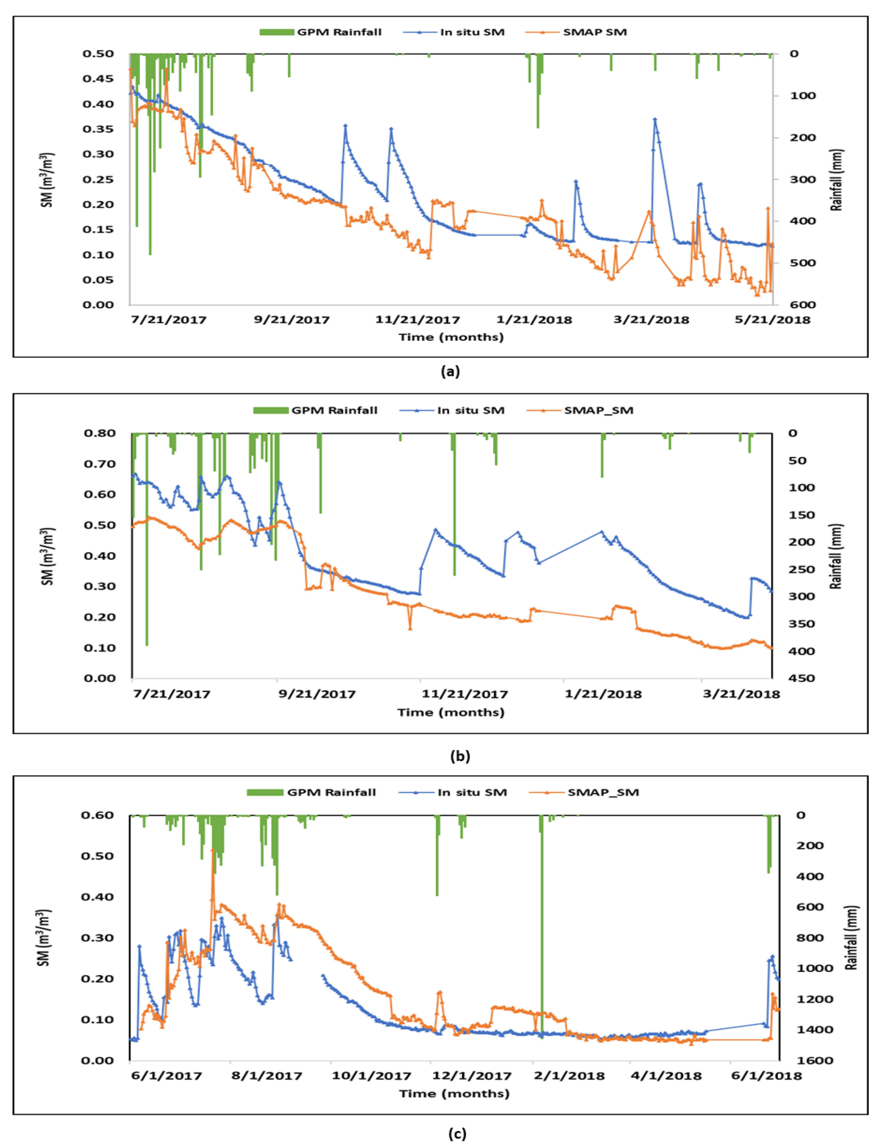
3.2.2. Temporal Consistency
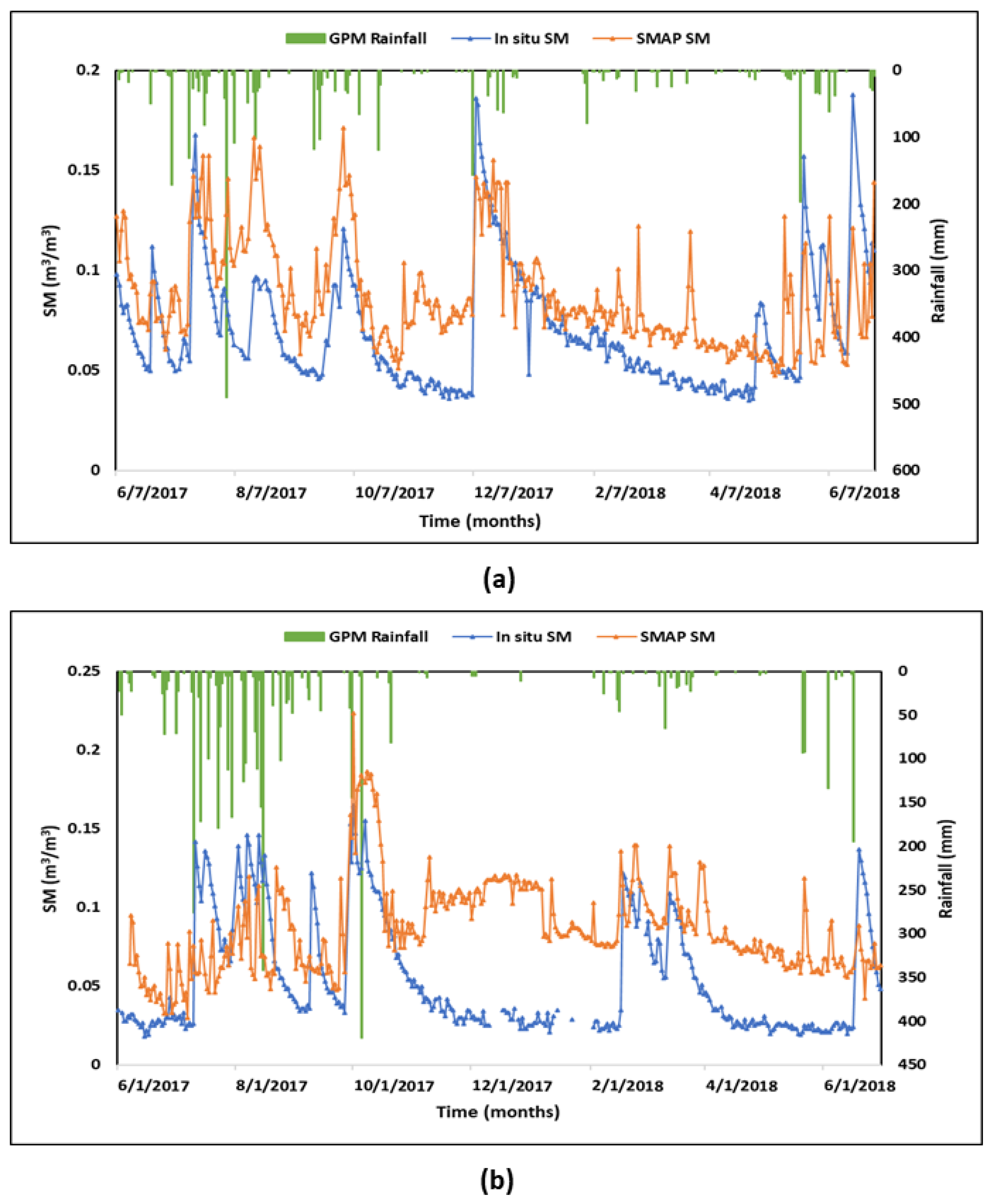
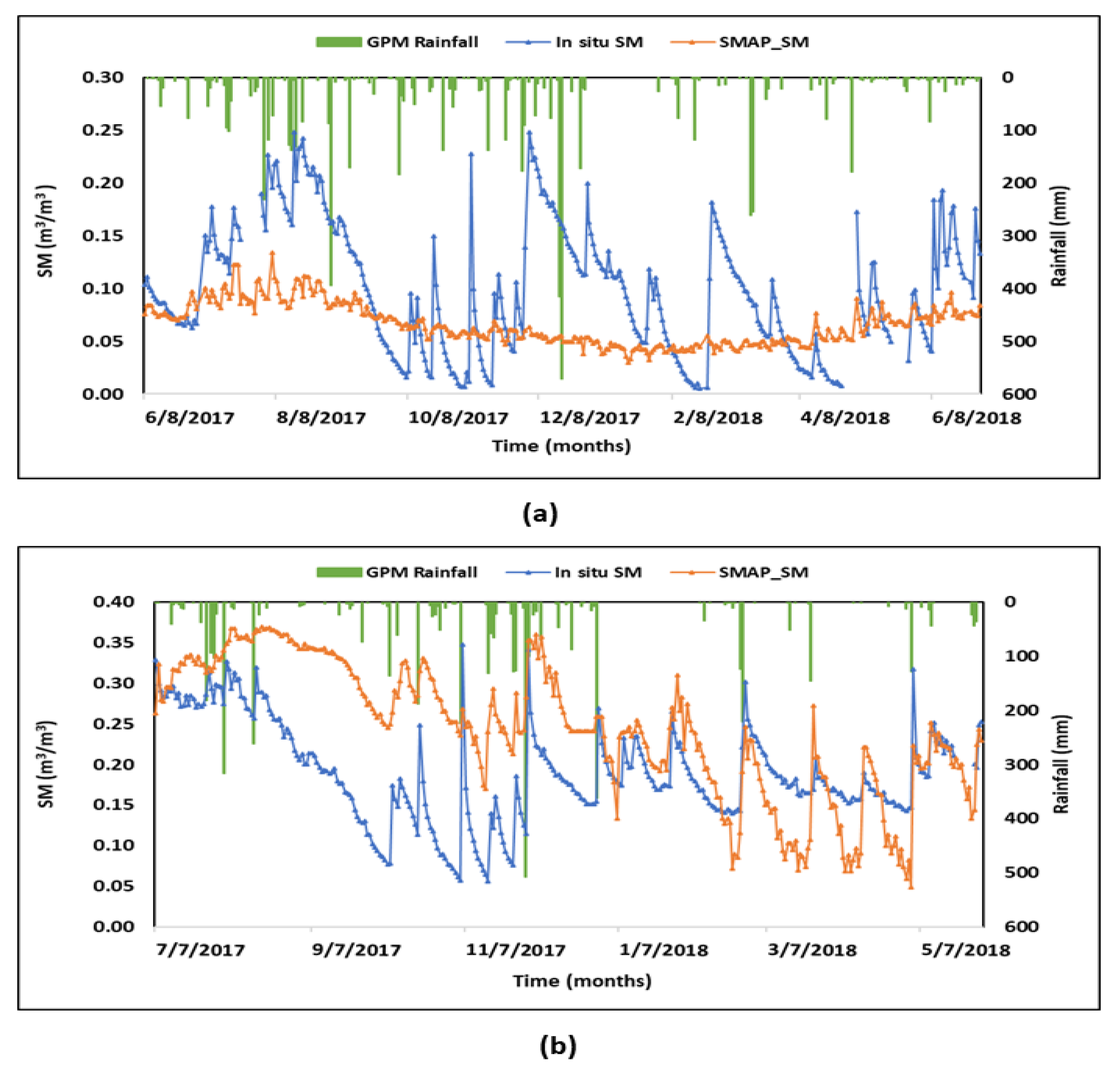
Figure 6a presents the temporal series plot for the Dumbraveni region, and the in situ data set obtained from the RSMN network. The negative PBIAS value (−59.30) indicated the overall underestimation of in situ SM measurements by the SMAP measurements. However, in the last phase of the study period during June 2018 both sets of data sets showed close agreement. The GPM estimates showed regular rainfall throughout the year except for January–March 2018 with no significant amount of rainfall. For the Feldbach region, Austria, Figure 6b represents the temporal series plot for the entire study period of one year (June 2017–July 2018) and the PBIAS value of 23.0 indicates an overestimation of in situ measurements by the satellite data set which is clearly shown in the plot. Overestimation was evident during the entire study period but a close approximation between the data sets during September, October and November 2017. At the last phase of the study period during May 2018, both the data sets showed close estimations. Like Dumbraveni, rainfall at Feldbach also showed significant presence throughout the study period except for January–March 2018. For El Coto, Spain, Figure 6c presents the temporal series plot. For the entire time period, the data sets show a significant underestimation (PBIAS = −78.50) of ground measurements from the satellite data set with not much variation in the latter except during a few days in October and November 2017, where the two data sets showed approximately similar estimates. Considerable amounts of rainfall were noticed during the months of June and December 2017 and April–June 2018. At El Coto, the ground-based sensor performed comparatively better than the air borne sensor in mapping of the SM variation with natural incoming moisture through rainfall.

3.3. Asia

3.3.1. Performance Comparison at Different Stations

An analysis was conducted to evaluate the SMAP SM product accuracy over the selected study sites in Asia. For the first site, Varanasi, Figure 7a shows the scatter plot between the satellite-derived, SMAP SM and in situ SM. Results of the statistical matrices calculated for both the data sets for the comparison showed a satisfactory agreement. For Varanasi the results obtained were R2 = 0.72, RMSE = 0.07, d = 0.88, PBIAS = −18.60. For the Hoshangabad region, Figure 7b presents the scatter plot between the SMAP and in situ SM data sets. The statistical scores also indicated a satisfactory performance of the SMAP SM product for this site with R2 = 0.71, RMSE = 0.14, d = 0.76, PBIAS = −29.60 indicating an underestimation by the SMAP product. For Anand, the two data sets showed a lower level of association compared to the previous two sites (R2 = 0.67). Results of another statistical score reported were RMSE = 0.07, d = 0.86 and PBIAS = 22.90. The PBIAS showed an overestimation at Anand. Based on the RMSE values between the SMAP SM product and ground-based SM measurements, the best performance was found at Varanasi (0.07) and Anand (0.07) and satisfactory at Hoshangabad (0.14). Results of d showed best match between the data set at Varanasi (0.88) followed by Anand (0.86) and Hoshangabad (0.76). The scatterplot for this site between both the data sets is presented in the Figure 7c below. Table 5 summarizes the results of the statistical tests for all three regions of the Asian subcontinent.

3.3.2. Temporal consistency
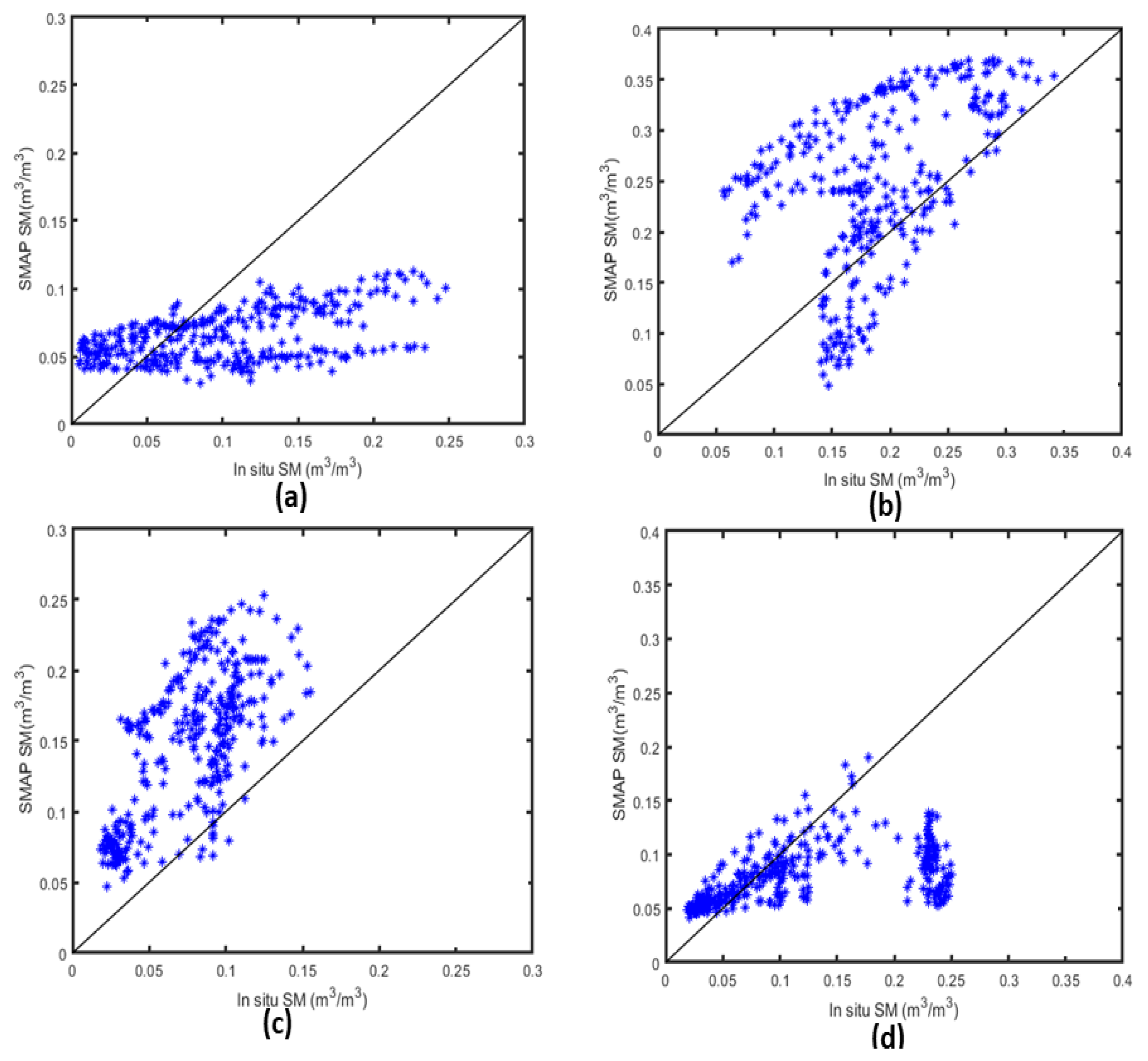
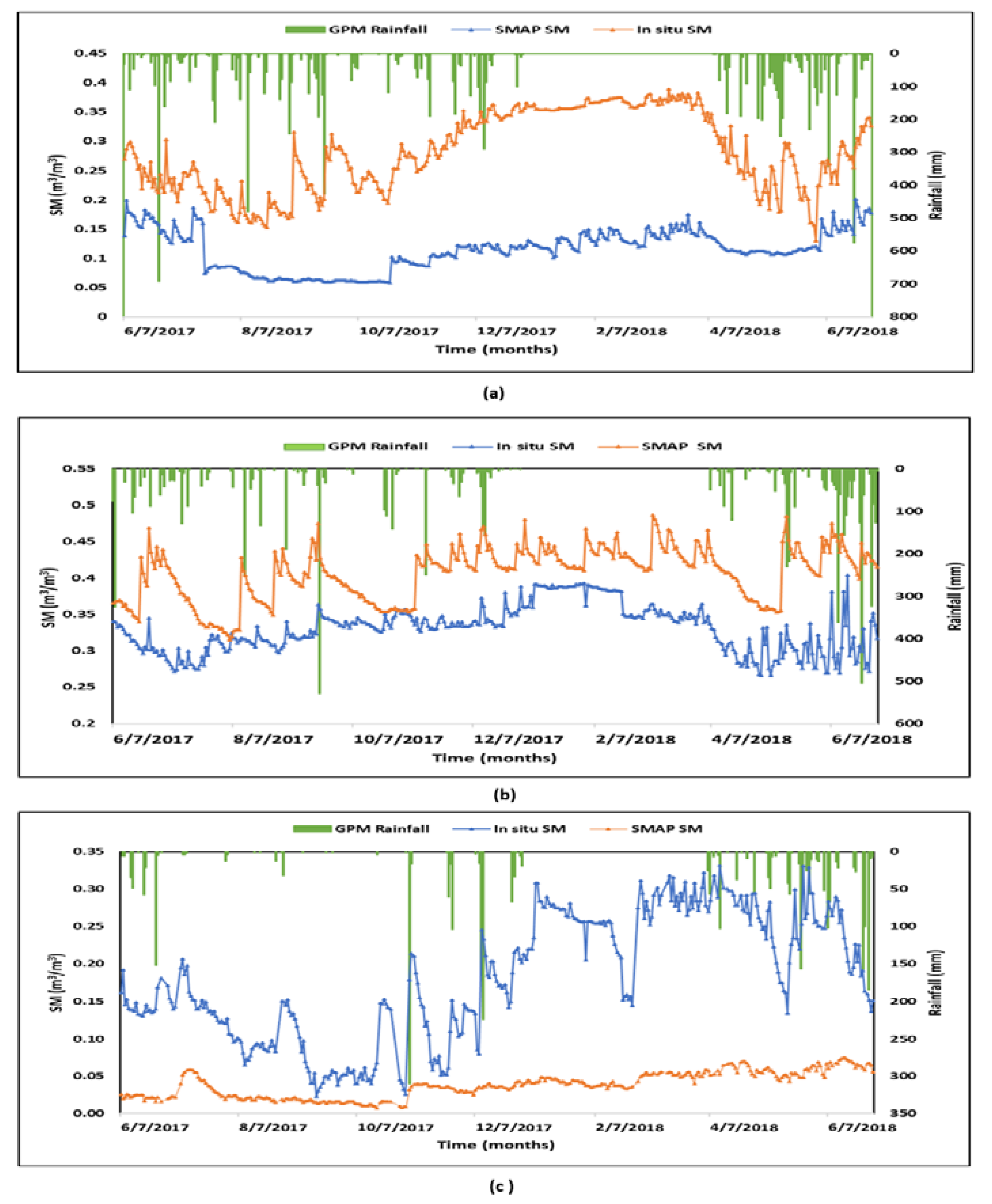
To explore the temporal trend between the SMAP SM and in situ SM data set for the Indian sites, a time series plot over the study period is shown in Figure 8 as these graphs help to analyze the overestimation or underestimation between the data sets. For the Varanasi site, the SMAP SM underestimated the ground-collected SM data set for most of the days during November (6–18 Nov) December (1–11), March and April by the SMAP SM. The time series plot is shown in Figure 8a for the Varanasi site. For Hoshangabad, the plot (Figure 8b) shows the variation between the data sets over the selected time period of this study. The PBIAS result (−29.60) indicated an overall underestimation of in situ observations by the SMAP SM product. However, the plot also showed an overestimating response of SMAP SM over a small period during mid-September (15–17 Sep) and mid-October (10–12 Oct.). For the Anand site, both the measurement techniques; in situ and satellite, showed the highest values of surface SM in the first phase of the study period, during July to September probably because of the monsoon season and significant amounts of rainfall prevailing in the area. SMAP SM showed a mixed kind of behavior of during this period. During June and July SMAP SM showed an underestimated behavior while for most of the time span it showed an overestimated measurement except for the last leg of study period, during the months of May and June 2018, the satellite measurement showed an underestimation. The temporal series plot for the Anand study is presented in Figure 8c. The rainfall pattern at all three selected sites showed the typical tropical monsoon type of climate of the Indian subcontinent with significant amounts of rainfall during the monsoon (June–September) and post-monsoon (October–November) seasons. The Varanasi site received a considerable amount of rainfall as can be seen during July–September 2017 and some during October 2017 and February and April 2018. At Hoshangabad, significant rainfall was observed during July–September 2017 and during few days in December 2017–January 2018 and February and March 2018. Rainfall at Anand also showed a similar pattern with the highest amount of rainfall during June–October 2017. However, a significant amount of rainfall can also be seen in December 2017 and January and February 2018.

3.4. Australia

3.4.1. Performance comparison at different stations

Results of the performance of the data sets is summarized in Table 6, while Figure 9a represents the scatterplot between the data sets for the Cox region and Figure 9b–d for the Samarra, Uri Park and Yanco regions, respectively. For the Australian continent, we selected four sites based on the availability of an in situ SM data set. The Uri Park site showed the highest correlation between the two data sets (R2 = 0.48, RMSE = 0.08, d = 0.49, PBIAS = 93.30) followed by Yanco (R2 = 0.29, RMSE = 0.08, d = 0.57, PBIAS = −31.60), the Cox region (R2 = 0.24, RMSE = 0.06, d = 0.53, PBIAS = −34.20) and Samarra (R2 = 0.19, RMSE = 0.1, d = 0.59, PBIAS = 28.90). Data sets at Samarra and Uri Park showed an overestimation while Cox and Yanco showed an underestimation. Comparison of performances among the sites, the SMAP SM performed best at Cox with the lowest RMSE value (0.06) followed by Uri Park (0.08), Yanco (0.08) and Samarra (0.10). Both the data sets showed best match at Samarra (0.59), Yanco (0.57), Cox (0.53) and least at Uri Park (0.49).

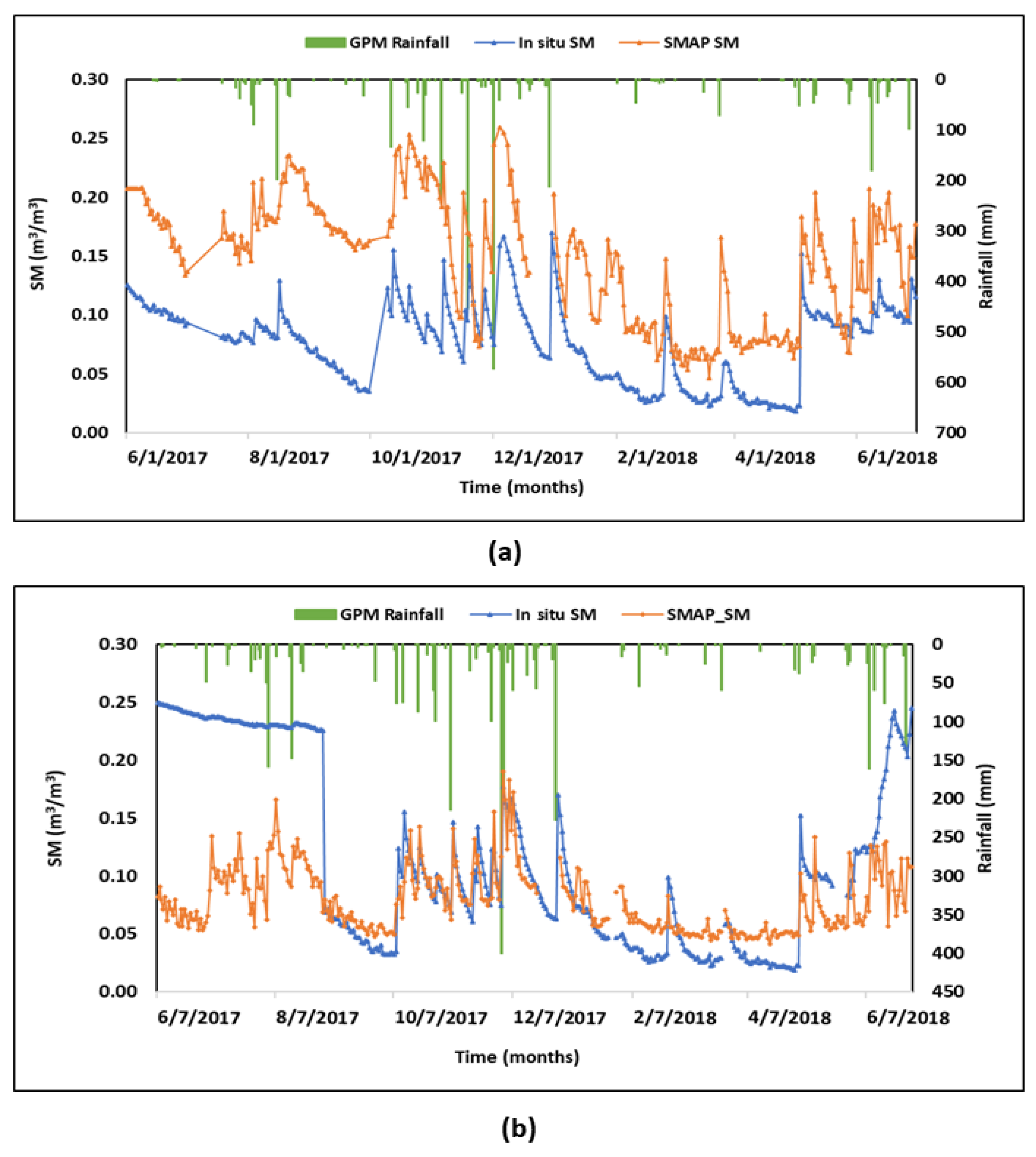
3.4.2. Temporal Consistency

For the Australian validation sites, Figure 10a presents the temporal series for the Cox site. The PBIAS value of −34.20 showed overall underestimation of the in situ data set by the SMAP SM estimates, however the time series plot revealed a mixed kind of association between the data sets. The in situ data set was noticeably higher than the satellite estimates in the first phase of the study period; during the months of July to October 2017, also during a few days in November and then a significant rise in the month of January 2018. This mixed pattern could be seen in the rest of the time period too. There was some discontinuity in the in situ data sets; during July–August 2017 and May–June 2018, that perhaps could be due to some technical fault in the sensor. Considerable amounts of rainfall could be noticed throughout the year with the maximum amount of rainfall during December 2017–January 2018. The response of the ground-measured SM to this fluctuation could be seen better than the satellite measured estimates at this site. For the Samarra region, Figure 10b shows the behavior of both the data sets over the study period. The PBIAS 28.90 showed an overestimation with a close association between the data sets. The graph showed a significant overestimation of in situ data set by the satellite data set from August to December 2017, however it is interesting to notice significant underestimation in the last phase of the study period, especially during the months of March to June 2018, by the SMAP data set.
Figure 11a represents the temporal plot between the data sets for Uri Park. The plot clearly depicted overestimation (PBIAS = 93.30) by the SMAP data set for the entire time span of this assessment period, however, a close association between the data sets could be noticed in the months of November–December 2017 and June–July 2018. At Yanco, the PBIAS value indicated an underestimation (PBIAS = −31.60) by the satellite. However, in the starting phase of the study period, from June to September 2017, the SMAP measurements clearly underestimated the in situ measurements, afterwards the data sets showed close approximation until June–July 2018, where ground-based estimates again overestimated the satellite measurements. There was also a gap in the ground-based data set in the months of June–July 2018. The temporal series plot for the Yanco site is presented in Figure 11b. At both the locations, maximum variation in both the SM data sets could be noticed on the days having notable amounts of rainfall which showed sensitivity of both these measurement techniques to the natural variation in SM. GPM rainfall at Uri Park showed significant amounts of rainfall during August–September 2017, December 2017–February 2018 and June–July 2018 with some dry periods in January–February 2018. Yanco received rainfall throughout the year except for a few days in January–February 2018 and highest during November 2017–January 2108.

4. Discussion

In this study, the performance of the SMAP L4 global SM data set across four continents was evaluated. This investigation also provides different insights into the sensitivity of in situ and satellite SM under different climatic and environmental conditions. Several authors (e.g., Chan et al. [53], Renzullo et al. [54], Bindlish et al. [55]) have already reported the utility of the ground-based SM estimates in assessing the quality and accuracy of satellite SM products. In this study, we used ground-based SM data sets from networks such as USCRN, RSMN, REMEDHUS, WEGENERNET, OZNET and the local SM networks in India to assess the performance of the SMAP L4 SM, a global surface and root zone SM product available at 3-h temporal and 9 km × 9 km spatial resolution. The results showed good performance of the SMAP SM products at most of the sites. The possible explanations for the poor performance of satellite SM at some locations could be as follows:
(1) Surface factors such as topographic complexities, vegetation density (size and growth stage), snow cover and volume scattering on dry soil playing a critical role in SM operational product retrieval accuracy [56,57,58,59]. Topographic features affect the accuracy and consistency of the retrieval process as surface conditions determine the microwave signatures [6]. With regard to the vegetation, vegetation structure and water content (VWC), if not accounted for properly, could strongly affect the quality of SM retrieval. The vegetation layer attenuates the microwave emissions from the surface and also contributes to the total radiation flux with its own emissions. VWC significantly affects the penetration of the microwave radiation. Engman and Chauhan [6] suggested that backscatter from a vegetated surface was affected by the variation in the VWC. Some authors [60,61] also suggested that the canopy layer was more transparent during day time and the summer months when the temperature was higher compared to night time and winter months. Therefore, to investigate the influence of these parameters on SM variation and performance of satellite SM in natural conditions, we selected validation sites for this study with different characteristics.
A possible explanation of the comparatively better performance of SMAP SM at the North American sites across the USCRN network could be due to the presence of a significant amount of bare soil and/or dry vegetation, uniform terrain and undisturbed locations. Similar results were also presented by Paredes and Barbosa [62] in their study conducted to compare the SMAP and SMOS SM product with in situ SM in northeast Brazil. Their assessment also found high correlation between the satellite and ground based SM estimates in the semi-arid regions with sparse vegetation but comparatively varying results for the rainy and forested regions of Amazonia and the Atlantic forests. Furthermore, seasonality is also considered an important factor regulating the SM variation. The role of seasonality in the performance of SMAP L4 SM product has been already foregrounded by Reichle et al. [63]. Climate and background environment played a vital role in satellite SM product performance particularly in the regions with extreme seasonal variability and fluctuating vegetation and surface conditions during growing and nongrowing seasons such as in India [64]. In this investigation, we found better performance of the SMAP SM product in the tropical climate of USA and in the subtropical steppe climate at Australian sites with oceanic influence, than in the humid subtropical climate of India and maritime temperate climate of Europe. The probable reason for these trends in results could be the presence of a considerable amount of sunshine with uniform rainfall throughout the year providing ideal conditions for the proper functioning and regulation of the hydrological cycle at the sites located in tropical and subtropical climates. In this study, to understand the SM variability at the selected validation sites, we used temporal plots between the SMAP SM, in situ SM and GPM rainfall data sets to represent the seasonal variation. From these plots for the USA sites (as shown in Figure 2, Figure 3 and Figure 4 ) the maximum SM variation was noticed during the growing season, specially, during spring (March–May) and summer (June–September) months due to the fluctuation in temperature and increased evapotranspiration activities, and minimum variation during the nongrowing season; the fall (October–November) and winter (December–February) months due to a comparatively lower temperature, snow and frozen soil conditions and less agricultural activities. For the European (Figure 5 and Figure 6) and Australian (Figure 9, Figure 10 and Figure 11) sites, SM variation could be noticed throughout the year with fluctuating temperature and regular periods of rainfall. However, for Indian sites (Figure 7 and Figure 8), frequent SM variations were noticed during summer (March–May), monsoon (June–September) and post-monsoon (October–November) than during the winter (December−February) months. In a study by Singh et al. [64], they investigated the SMAP product performance in the paddy sown fields. The author also suggested that one of the ways to improve satellite SM retrieval globally could be by assessing the satellite product performance in different parts of the world with varying seasonal and soil conditions.
(2) Spatial mismatch between the ground and satellite estimates of SM can cause deviation and error. Since ground-based point measurements could not represent the SM at the same spatial scale within the large footprint of the satellite product, the averaged SM value was often represented as the reference value. Many studies [18,32] have suggested that point-based measurements can only represent the temporal dynamics of the SM but not the absolute value. This can only be achieved by upscaling the point estimates using techniques proposed by [24]. Dense, in situ networks are very useful in this regard.
(3) Error caused by the measurement accuracy of the sensors. Even though ground-based SM networks seemed to provide a wealth of knowledge, the in situ data set contained a significant amount of errors due to both instrumental and representational issues, mostly due to the difference in the measurement method, installation depths and modes, calibration techniques, data set uniformity, measurement intervals and lack of proper maintenance. These factors are also believed to have a significant impact on calibration and validation of satellite SM products.
The overall results of this study suggest that the agreement between the satellite and ground-based SM measurements could be affected by sensor sensitivity, penetration power, spatial resolution, land surface factors (such as topography, land cover types, etc.), intracontinental differences and seasonal variations [31,65,66]. The SM conditions potentially depend on the weather conditions and phenological changes in the vegetation, growth stages, size density and water content that may attenuate the microwave signals and reduce the overall accuracy of the retrieval. This study emphasizes the need for more assessment studies like these to understand applicability of the SMAP product utilities and its performance over different landscapes. This study also offers a promising approach for the scope and wider applications of SM retrieval algorithms, using brightness temperature-based radiative transfer models and disaggregation techniques for more precise estimations at finer spatial scale.

5. Conclusions

SMAP is the latest and one of the most sophisticated satellite missions for monitoring global SM change across the globe. However, like any other satellite product, the applications and limitations of the SMAP products also need to be assessed and validated and studies like this help in getting a better insight into the performance and applicability of SMAP for precise and frequent global SM monitoring. With the purpose to understand the SMAP SM product quality and utility, this study aimed at assessing the performance of the SMAP L4 global SM product at selected validation sites across four continents having different climates, land covers and soil types and also to understand the role and limitations of ground-based measurements in the process.
The results of our study showed that SM variation is very much dependent on terrain, geographical feature and seasonal variation of the location and many more studies like this assessing the product quality of SMAP should be conducted to make the users aware of the uncertainties associated with the satellite data sets. The overall results of the comparison between the satellite and in situ SM estimates showed good performance of the SMAP in capturing the near surface (0−5 cm) SM variations. The low value of RMSE (usually near 0.04 m3/m3) suggests that the SMAP SM product provides valuable information about the SM variation under various land covers, climatic regions and soil types. The SMAP SM showed good agreement with the in situ measurements at most of the sites. At some of the sites the SMAP SM showed an overestimation and high RMSE which suggested the vegetation effect on the sensor-based SM product should be accounted for properly to achieve accurate and precise estimations. The performance of satellite SM is relatively lower during the winter months of the year, which could be because of the complexities due to frozen soil and snow cover at the locations. Results also suggest that even though satellite SM products are performing satisfactorily in capturing the surface SM variation in natural ecosystems, more assessments like this are needed to increase the practical application of sensor-based global SM products.
However, the major issue inherent with the validation of satellite SM products is the spatial scale of the ground-based observations. A dense network of in situ stations are often substantially lacking in studies like these. For proper validation, quality-controlled sites are needed, having large homogenous field conditions, maintained in situ observations, easy and continuous availability of in situ data sets, having proper descriptions of the sites, etc. Nevertheless, a greater number of sensors if available are always good to reduce uncertainty in validation studies.
In future, more precise prediction of SM with integration of numerical weather models, hydrological models and meteorological variables will be attempted that could be crucial in more accurately understanding the behavior and variation of SM in natural landscape at the local, regional and global scale.

Author Contributions

Conceptualization, P.K.S. data set curation, S.S., D.K.P. and P.E.O.; formal analysis, S.S.; funding acquisition, P.K.S.; investigation, P.K.S.; methodology, P.K.S. and S.S.; project administration, P.K.S.; resources, P.K.S., G.P.P. and D.K.P. software, P.K.S. and S.S.; supervision, P.K.S.; validation, S.S. and P.E.O. visualization, G.P.P.; writing—original draft, P.K.S. and S.S.; writing—review and editing, P.K.S., G.P.P. and P.E.O. All authors have read and agreed to the published version of the manuscript.

Funding

S.S.’s contribution was supported by the University Grant Commission and Banaras Hindu University, India. P.K.S.’s, contribution was supported by the Space Application Centre, ISRO, India. G.P.P.’s participation was supported financially by the European Union’s Horizon 2020 Marie Skłodowska-Curie Project “ENViSIoN-EO” (grant agreement No 752094).

Acknowledgments

We thank all the in situ data set providers for making their data set available from USCRN, RSMN, REMEDHUS, WEGENERNET and OZNET networks through ISMN. The authors would also like to thank the Space Applications Center (SAC), Indian Space Research Organization (ISRO), India for providing in situ data over Indian sites and their funding. The authors wish to also thank the editor and the anonymous reviewers for their constructive comments and feedback for improving this manuscript.

Conflicts of Interest

The authors declare no conflict of interest.

References

  1. Piles, M.; Petropoulos, G.P.; Sánchez, N.; González-Zamora, Á.; Ireland, G. Towards improved spatio-temporal resolution soil moisture retrievals from the synergy of SMOS and MSG SEVIRI spaceborne observations. Remote Sens. Environ. 2016, 180, 403–417. [Google Scholar] [CrossRef] [Green Version]
  2. Carlson, T.N.; Petropoulos, G.P. A new method for estimating of evapotranspiration and surface soil moisture from Optical and Thermal Infrared measurements: The simplified triangle. Int. J. Remote Sens. 2019, 40, 7716–7729. [Google Scholar] [CrossRef]
  3. Srivastava, P.K.; Han, D.; Ramirez, M.R.; Islam, T. Appraisal of SMOS soil moisture at a catchment scale in a temperate maritime climate. J. Hydrol. 2013, 498, 292–304. [Google Scholar] [CrossRef]
  4. Njoku, E.G.; Entekhabi, D. Passive microwave remote sensing of soil moisture. J. Hydrol. 1996, 184, 101–129. [Google Scholar] [CrossRef]
  5. Srivastava, P.K.; Han, D.; Rico-Ramirez, M.A.; O’Neill, P.; Islam, T.; Gupta, M.; Dai, Q. Performance evaluation of WRF-NOAH Land Surface Model estimated soil moisture for hydrological application: Synergistic evaluation using SMOS retrieved soil moisture. J. Hydrol. 2015, 529, 200–212. [Google Scholar] [CrossRef]
  6. Engman, E.T.; Chauhan, N. Status of microwave soil moisture measurements with remote sensing. Remote Sens. Environ. 1995, 51, 189–198. [Google Scholar] [CrossRef]
  7. Srivastava, P.; O’Neill, P.; Cosh, M.; Kurum, M.; Lang, R.; Joseph, A. Evaluation of dielectric mixing models for passive microwave soil moisture retrieval using data from comrad ground-based SMAP simulator. IEEE J. Sel. Top. Appl. Earth Obs. Remote Sens. 2014, 8, 4345–4354. [Google Scholar] [CrossRef]
  8. Choi, M.; Hur, Y. A microwave-Optical/Infrared disaggregation for improving spatial representation of soil moisture using AMSR-E and MODIS products. Remote Sens. Environ. 2012, 124, 259–269. [Google Scholar] [CrossRef]
  9. Srivastava, P.K.; Yaduvanshi, A.; Singh, S.K.; Islam, T.; Gupta, M. Support vector machines and generalized linear models for quantifying soil dehydrogenase activity in agro-forestry system of mid altitude Central Himalaya. Environ. Earth Sci. 2016, 75, 299. [Google Scholar] [CrossRef]
  10. Deng, K.A.K.; Lamine, S.; Pavlides, A.; Petropoulos, G.P.; Bao, Y.; Srivastava, P.K.; Guan, Y. Large scale operational soil moisture mapping from passive MW radiometry: SMOS product evaluation in Europe & USA. Int. J. Appl. Earth Obs. Geoinf. 2019, 80, 206–217. [Google Scholar]
  11. Tian, X.; Xie, Z.; Dai, A.; Shi, C.; Jia, B.; Chen, F.; Yang, K. A dual-pass variational data assimilation framework for estimating soil moisture profiles from AMSR-E microwave brightness temperature. J. Geophys. Res. Atmos. 2009, 114, 1–12. [Google Scholar] [CrossRef] [Green Version]
  12. Fuzzo, D.F.S.; Carlson, T.N.; Kourgialas, N.N.; Petropoulos, G.P. Coupling remote sensing with a water balance model for soybean yield predictions over large areas. Earth Sci. Inform. 2019, 13, 345–359. [Google Scholar] [CrossRef]
  13. Bao, Y.; Lin, L.; Wu, S.; Deng, K.A.K.; Petropoulos, G.P. Surface soil moisture retrievals over partially vegetated areas from the synergy of Sentinel-1 and Landsat 8 data using a modified Water-Cloud model. Int. J. Appl. Earth Obs. Geoinf. 2018, 72, 76–85. [Google Scholar] [CrossRef]
  14. Laymon, C.A.; Manu, A.; Crosson, W.L.; Jackson, T.J. Defining the range of uncertainty associated with remotely sensed soil moisture estimates with microwave radiometers. In Remote Sensing for Earth Science, Ocean, and Sea Ice Applications; SPIE Digital Library: Bellingham, DC, USA, 1999; pp. 504–513. [Google Scholar]
  15. Gupta, M.; Srivastava, P.K.; Islam, T.; Ishak, A.M.B. Evaluation of TRMM rainfall for soil moisture prediction in a subtropical climate. Environ. Earth Sci. 2013. [Google Scholar] [CrossRef]
  16. Srivastava, P.K.; Han, D.; Rico-Ramirez, M.A.; O’Neill, P.; Islam, T.; Gupta, M. Assessment of SMOS soil moisture retrieval parameters using tau–omega algorithms for soil moisture deficit estimation. J. Hydrol. 2014, 519, 574–587. [Google Scholar] [CrossRef] [Green Version]
  17. Srivastava, P.K.; Han, D.; Rico-Ramirez, M.A.; Al-Shrafany, D.; Islam, T. Data fusion techniques for improving soil moisture deficit using SMOS satellite and WRF-NOAH Land Surface Model. Water Resour. Manag. 2013, 27, 5069–5087. [Google Scholar] [CrossRef]
  18. Wagner, W.; Hahn, S.; Kidd, R.; Melzer, T.; Bartalis, Z.; Hasenauer, S.; Figa-Saldaña, J.; de Rosnay, P.; Jann, A.; Schneider, S. The ASCAT soil moisture product: A review of its specifications, validation results, and emerging applications. Meteorol. Z. 2013, 22, 5–33. [Google Scholar] [CrossRef] [Green Version]
  19. Njoku, E.G.; Jackson, T.J.; Lakshmi, V.; Chan, T.K.; Nghiem, S.V. Soil moisture retrieval from AMSR-E. IEEE Trans. Geosci. Remote Sens. 2003, 41, 215–229. [Google Scholar] [CrossRef]
  20. Imaoka, K.; Maeda, T.; Kachi, M.; Kasahara, M.; Ito, N.; Nakagawa, K. Earth Observing Missions and Sensors: Development, Implementation, and Characterization II. In Status of AMSR2 Instrument on GCOM-W1; SPIE Digital Library: Bellingham, DC, USA, 2012; p. 852815. [Google Scholar]
  21. Kerr, Y.H.; Waldteufel, P.; Wigneron, J.-P.; Delwart, S.; Cabot, F.; Boutin, J.; Escorihuela, M.-J.; Font, J.; Reul, N.; Gruhier, C. The SMOS mission: New tool for monitoring key elements ofthe global water cycle. Proc. IEEE 2010, 98, 666–687. [Google Scholar] [CrossRef] [Green Version]
  22. Entekhabi, D.; Njoku, E.G.; O’Neill, P.E.; Kellogg, K.H.; Crow, W.T.; Edelstein, W.N.; Entin, J.K.; Goodman, S.D.; Jackson, T.J.; Johnson, J. The Soil Moisture Active Passive (SMAP) mission. Proc. IEEE 2010, 98, 704–716. [Google Scholar] [CrossRef]
  23. Srivastava, P.K.; Petropoulos, G.; Kerr, Y.H. Satellite Soil Moisture Retrieval: Techniques and Applications; Elsevier: Amsterdam, The Netherlands, 2016; ISBN 9780128033883. [Google Scholar]
  24. Srivastava, P.K. Satellite soil moisture: Review of theory and applications in water resources. Water Resour. Manag. 2017, 31, 3161–3176. [Google Scholar] [CrossRef]
  25. Tebbs, E.; Wilson, H.; Mulligan, M.; Chan, K.; Gupta, M.; Maurya, V.; Srivastava, P. Satellite soil moisture observations: Applications in the UK and India. In Report of Pump Priming Project the India-UK Water Centre; Wallingford and Pune: Dehradun, India, 2019. [Google Scholar]
  26. Srivastava, P.K.; Pandey, P.C.; Petropoulos, G.P.; Kourgialas, N.N.; Pandey, V.; Singh, U. GIS and remote sensing aided information for soil moisture estimation: A comparative study of interpolation techniques. Resources 2019, 8, 70. [Google Scholar] [CrossRef] [Green Version]
  27. Srivastava, P.K.; Pandey, P.C.; Kumar, P.; Raghubanshi, A.S.; Han, D. Geospatial Technology for Water Resource Applications; CRC Press: Boca Raton, FL, USA; Taylor and Francis: Abingdon, UK, 2016; ISBN 9781498719681. [Google Scholar]
  28. Srivastava, P.K.; Han, D.; Ramirez, M.R.; Islam, T. Machine learning techniques for downscaling SMOS satellite soil moisture using MODIS Land Surface Temperature for hydrological application. Water Resour. Manag. 2013, 27, 3127–3144. [Google Scholar] [CrossRef]
  29. Deng, K.A.K.; Lamine, S.; Pavlides, A.; Petropoulos, G.P.; Srivastava, P.K.; Bao, Y.; Hristopulos, D.; Anagnostopoulos, V. Operational soil moisture from ASCAT in support of water resources management. Remote Sens. 2019, 11, 579. [Google Scholar] [CrossRef] [Green Version]
  30. Dobriyal, P.; Qureshi, A.; Badola, R.; Hussain, S.A. A review of the methods available for estimating soil moisture and its implications for water resource management. J. Hydrol. 2012, 458, 110–117. [Google Scholar] [CrossRef]
  31. Petropoulos, G.P.; Ireland, G.; Srivastava, P.K.; Ioannou-Katidis, P. An appraisal of the accuracy of operational soil moisture estimates from SMOS MIRAS using validated in situ observations acquired in a mediterranean environment. Int. J. Remote Sens. 2014, 35, 5239–5250. [Google Scholar] [CrossRef]
  32. Petropoulos, G.P.; Ireland, G.; Srivastava, P.K. Evaluation of the soil moisture operational estimates from SMOS in Europe: Results over diverse ecosystems. IEEE Sens. J. 2015, 15, 5243–5251. [Google Scholar] [CrossRef]
  33. Petropoulos, G.P.; McCalmont, J.P. An operational in situ soil moisture & soil temperature monitoring network for West Wales, UK: The WSMN network. Sensors 2017, 17, 1481. [Google Scholar]
  34. Petropoulos, G.; Srivastava, P.K.; Ferentinos, K.P.; Hristopoulos, D. Evaluating the capabilities of Optical/TIR imaging sensing systems for quantifying soil water content. Geocarto Int. 2018, 35, 494–511. [Google Scholar] [CrossRef]
  35. Dorigo, W.; Wagner, W.; Hohensinn, R.; Hahn, S.; Paulik, C.; Xaver, A.; Gruber, A.; Drusch, M.; Mecklenburg, S.; Oevelen, P.V. The International Soil Moisture Network: A data hosting facility for global in situ soil moisture measurements. Hydrol. Earth Syst. Sci. 2011, 15, 1675–1698. [Google Scholar] [CrossRef] [Green Version]
  36. Diamond, H.J.; Karl, T.R.; Palecki, M.A.; Baker, C.B.; Bell, J.E.; Leeper, R.D.; Easterling, D.R.; Lawrimore, J.H.; Meyers, T.P.; Helfert, M.R. US Climate Reference Network after one decade of operations: Status and assessment. Bull. Am. Meteorol. Soc. 2013, 94, 485–498. [Google Scholar] [CrossRef]
  37. Stancalie, G.; Catana, S.; Irimescu, A.; Savin, E.; Diamandi, A.; Hofnar, A.; Oancea, S. Contribution of earth observation data supplied by the new satellite sensors to flood management. In Transboundary Floods: Reducing Risks Through Flood Management; Springer: Berlin/Heidelberg, Germany, 2006; pp. 287–304. [Google Scholar]
  38. Moe, K.H.; Dwolatzky, B.; Olst, R. Designing a Usable Mobile Application for Field Data Collection. In Proceedings of the 2004 IEEE Africon. 7th Africon Conference in Africa (IEEE Cat. No. 04CH37590), Gaborone, Botswana, 15–17 September 2004; pp. 1187–1192. [Google Scholar]
  39. Kirchengast, G.; Kabas, T.; Leuprecht, A.; Bichler, C.; Truhetz, H. Wegenernet: A pioneering high-resolution network for monitoring weather and climate. Bull. Am. Meteorol. Soc. 2014, 95, 227–242. [Google Scholar] [CrossRef]
  40. Smith, A.B.; Walker, J.P.; Western, A.W.; Young, R.; Ellett, K.; Pipunic, R.; Grayson, R.; Siriwardena, L.; Chiew, F.H.; Richter, H. The Murrumbidgee soil moisture monitoring network data set. Water Resour. Res. 2012, 7, 1–6. [Google Scholar] [CrossRef]
  41. Cosh, M.H.; Ochsner, T.E.; McKee, L.; Dong, J.; Basara, J.B.; Evett, S.R.; Hatch, C.E.; Small, E.E.; Steele-Dunne, S.C.; Zreda, M. The Soil Moisture Active Passive Marena, Oklahoma, in situ sensor testbed (SMAP-MOISST): Testbed design and evaluation of in situ sensors. Vadose Zone J. 2016, 15, 1–11. [Google Scholar] [CrossRef] [Green Version]
  42. Chen, F.; Crow, W.T.; Colliander, A.; Cosh, M.H.; Jackson, T.J.; Bindlish, R.; Reichle, R.H.; Chan, S.K.; Bosch, D.D.; Starks, P.J. Application of triple collocation in ground-based validation of Soil Moisture Active/Passive (SMAP) level 2 data products. IEEE J. Sel. Topics Appl. Earth Obs. Remote Sens. 2016, 10, 489–502. [Google Scholar] [CrossRef]
  43. Wu, C.-C.; Margulis, S.A. Real-time soil moisture and salinity profile estimation using assimilation of embedded sensor datastreams. Vadose Zone J. 2013, 12, 1–17. [Google Scholar] [CrossRef]
  44. Colliander, A.; Cosh, M.H.; Misra, S.; Jackson, T.J.; Crow, W.T.; Chan, S.; Bindlish, R.; Chae, C.; Collins, C.H.; Yueh, S.H. Validation and scaling of soil moisture in a semi-arid environment: SMAP validation experiment 2015 (SMAPVEX15). Remote Sens. Environ. 2017, 196, 101–112. [Google Scholar] [CrossRef]
  45. Entekhabi, D.; Yueh, S.; O’Neill, P.E.; Kellogg, K.H.; Allen, A.; Bindlish, R.; Brown, M.; Chan, S.; Colliander, A.; Crow, W.T. SMAP Handbook–Soil Moisture Active Passive: Mapping Soil Moisture and Freeze/Thaw from Space; JPL Publication: Pasadena, CA, USA, 2014. [Google Scholar]
  46. Entekhabi, D.; Yueh, S.; De Lannoy, G. SMAP Handbook; JPL Publication: Pasadena, CA, USA, 2014. [Google Scholar]
  47. Chaubell, M.J.; Yueh, S.H.; Dunbar, R.S.; Colliander, A.; Chen, F.; Chan, S.K.; Entekhabi, D.; Bindlish, R.; O’Neill, P.E.; Asanuma, J. Improved SMAP dual-channel algorithm for the retrieval of soil moisture. IEEE Trans. Geosci. Remote Sens. 2020, 58, 3894–3905. [Google Scholar] [CrossRef]
  48. Huffman, G.J.; Bolvin, D.T.; Braithwaite, D.; Hsu, K.; Joyce, R.; Xie, P.; Yoo, S.-H. NASA Global Precipitation Measurement (GPM) Integrated Multi-Satellite Retrievals for GPM (IMERG). Algorithm Theor. Basis Doc. (ATBD) Version 2015, 4, 26. [Google Scholar]
  49. Huffman, G.J.; Bolvin, D.T.; Nelkin, E.J. Day 1 IMERG Final Run Release Notes; NASA/GSFC: Greenbelt, MD, USA, 2015. [Google Scholar]
  50. Willmott, C.J. On the validation of models. Phys. Geogr. 1981, 2, 184–194. [Google Scholar] [CrossRef]
  51. Willmott, C.J. Some comments on the evaluation of model performance. Bull. Am. Meteorol. Soc. 1982, 63, 1309–1313. [Google Scholar] [CrossRef] [Green Version]
  52. Legates, D.R.; McCabe, G.J., Jr. Evaluating the use of “goodness-of-fit” measures in hydrologic and hydroclimatic model validation. Water Resour. Res. 1999, 35, 233–241. [Google Scholar] [CrossRef]
  53. Chan, S.K.; Bindlish, R.; O’Neill, P.E.; Njoku, E.; Jackson, T.; Colliander, A.; Chen, F.; Burgin, M.; Dunbar, S.; Piepmeier, J. Assessment of the SMAP passive soil moisture product. IEEE Trans. Geosci. Remote Sens. 2016, 54, 4994–5007. [Google Scholar] [CrossRef]
  54. Renzullo, L.J.; Van Dijk, A.; Perraud, J.-M.; Collins, D.; Henderson, B.; Jin, H.; Smith, A.; McJannet, D. Continental satellite soil moisture data assimilation improves root-zone moisture analysis for water resources assessment. J. Hydrol. 2014, 519, 2747–2762. [Google Scholar] [CrossRef]
  55. Bindlish, R.; Jackson, T.; Cosh, M.; Zhao, T.; O’Neill, P. Global soil moisture from the Aquarius/SAC-D satellite: Description and initial assessment. IEEE Geosci. Remote Sens. Lett. 2015, 12, 923–927. [Google Scholar] [CrossRef]
  56. Zhang, C.; Cheng, Q.; Yang, J.; Zhao, J.; Cui, T.J. Broadband metamaterial for optical transparency and microwave absorption. Appl. Phys. Lett. 2017, 110, 143511. [Google Scholar] [CrossRef]
  57. Colliander, A.; Jackson, T.J.; Bindlish, R.; Chan, S.; Das, N.; Kim, S.; Cosh, M.; Dunbar, R.; Dang, L.; Pashaian, L. Validation of SMAP surface soil moisture products with core validation sites. Remote Sens. Environ. 2017, 191, 215–231. [Google Scholar] [CrossRef]
  58. El Hajj, M.; Baghdadi, N.; Zribi, M.; Rodríguez-Fernández, N.; Wigneron, J.P.; Al-Yaari, A.; Al Bitar, A.; Albergel, C.; Calvet, J.-C. Evaluation of SMOS, SMAP, ASCAT and Sentinel-1 soil moisture products at sites in southwestern France. Remote Sens. 2018, 10, 569. [Google Scholar] [CrossRef] [Green Version]
  59. Liu, Y.Y.; de Jeu, R.A.; McCabe, M.F.; Evans, J.P.; van Dijk, A.I. Global long-term passive microwave satellite-based retrievals of vegetation optical depth. Geophys. Res. Lett. 2011, 38, 1–6. [Google Scholar] [CrossRef] [Green Version]
  60. Brocca, L.; Hasenauer, S.; Lacava, T.; Melone, F.; Moramarco, T.; Wagner, W.; Dorigo, W.; Matgen, P.; Martínez-Fernández, J.; Llorens, P. Soil moisture estimation through ASCAT and AMSR-E sensors: An intercomparison and validation study across Europe. Remote Sens. Environ. 2011, 115, 3390–3408. [Google Scholar] [CrossRef]
  61. Chen, Y.; Yang, K.; Qin, J.; Zhao, L.; Tang, W.; Han, M. Evaluation of AMSR-E retrievals and GLDAS simulations against observations of a soil moisture network on the central tibetan plateau. J. Geophys. Res. Atmos. 2013, 118, 4466–4475. [Google Scholar] [CrossRef]
  62. Paredes-Trejo, F.; Barbosa, H. Evaluation of the SMOS-derived soil water deficit index as agricultural drought index in northeast of Brazil. Water 2017, 9, 377. [Google Scholar] [CrossRef]
  63. Reichle, R.H.; De Lannoy, G.J.; Liu, Q.; Ardizzone, J.V.; Colliander, A.; Conaty, A.; Crow, W.; Jackson, T.J.; Jones, L.A.; Kimball, J.S. Assessment of the SMAP level-4 surface and root-zone soil moisture product using in situ measurements. J. Hydrometeorol. 2017, 18, 2621–2645. [Google Scholar] [CrossRef]
  64. Singh, G.; Das, N.N.; Panda, R.K.; Colliander, A.; Jackson, T.J.; Mohanty, B.P.; Entekhabi, D.; Yueh, S.H. Validation of SMAP soil moisture products using ground-based observations for the paddy dominated tropical region of India. IEEE Trans. Geosci. Remote Sens. 2019, 57, 8479–8491. [Google Scholar] [CrossRef]
  65. Pierdicca, N.; Pulvirenti, L.; Fascetti, F.; Crapolicchio, R.; Talone, M. Analysis of two years of ASCAT-and SMOS-derived soil moisture estimates over Europe and North Africa. Eur. J. Remote Sens. 2013, 46, 759–773. [Google Scholar] [CrossRef]
  66. Dorigo, W.; Xaver, A.; Vreugdenhil, M.; Gruber, A.; Hegyiova, A.; Sanchis-Dufau, A.; Zamojski, D.; Cordes, C.; Wagner, W.; Drusch, M. Global automated quality control of in situ soil moisture data from the International Soil Moisture Network. Vadose Zone J. 2013, 1–12. [Google Scholar] [CrossRef]
Figure 1. Locations of the validation sites used in this study; 1. Fallbrook, California, USA, 2. Tucson, Arizona, USA, 3. Socorro, Minnesota, USA, 4. Panther Junction, Texas, USA, 5. El Coto, Spain, 6. Feldbach, Austria, 7. Dumbraveni, Romania, 8. Anand, Gujarat, India, 9. Hoshangabad, M.P. India, 10. Varanasi, U.P. India, 11. Cox, Australia, 12. Uri Park, Australia, 13. Yanco, Australia, 14. Samarra, Australia.
Remotesensing 12 01977 g001
Figure 2. Comparisons between the soil moisture active passive (SMAP) SM and in situ soil moisture (SM) for (a) Fallbrook, California, (b) Tucson, Arizona, (c) Panther Junction, Texas and (d) Socorro, Minnesota, North America.
Remotesensing 12 01977 g002
Figure 3. Temporal series plot between the SMAP SM, in situ SM and GPM rainfall for (a) Fallbrook, California and (b) Tucson, Arizona, North America.
Remotesensing 12 01977 g003
Figure 4. Temporal series plot between the SMAP SM, in situ SM and GPM rainfall for (a) Panther Junction, Texas and (b) Socorro, Minnesota, North America.
Remotesensing 12 01977 g004
Figure 5. Comparisons between the SMAP SM and in situ SM for (a) Dumbraveni, Romania (b) Feldbach, Austria and (c) El Coto, Spain, Europe.
Remotesensing 12 01977 g005
Figure 6. Temporal series plot between the SMAP SM, in situ SM and GPM rainfall for (a) Dumbraveni, Romania (b) Feldbach, Austria and (c) El Coto, Spain, Europe.
Remotesensing 12 01977 g006
Figure 7. Comparisons between the SMAP SM and in situ SM for (a) Varanasi, Uttar Pradesh (b) Hoshangabad, Madhya Pradesh and (c) Anand, Gujarat, India, Asia.
Remotesensing 12 01977 g007
Figure 8. Temporal plot between the SMAP SM, in situ SM and GPM rainfall for (a) Varanasi, Uttar Pradesh (b) Hoshangabad, Madhya Pradesh and (c) Anand, Gujarat, India, Asia.
Remotesensing 12 01977 g008
Figure 9. Comparisons between the SMAP SM and in situ SM for (a) Cox (b) Samarra (c) Uri Park and (d) Yanco, Australia.
Remotesensing 12 01977 g009
Figure 10. Temporal series plot between the SMAP SM, in situ SM and GPM rainfall for (a) Cox and (b) Samarra, Australia.
Remotesensing 12 01977 g010
Figure 11. Temporal series plots between the SMAP SM, in situ SM and GPM rainfall for (a) Uri Park and (b) Yanco, Australia.
Remotesensing 12 01977 g011
Table 1. Characteristics of the main ground observational networks used in our study.
LocationISMN Network SensorSoil DepthParameters
North America
(USA)
USCRNStevens Water Inc.
Stevens Hydra Probe II
0–0.05 m
0.05–0.1 m
0.1–0.2 m
0.2–0.5 m
0.5–1.0 m
Soil moisture, soil temperature, precipitation, air temperature, surface temperature.
Europe
(Dumbraveni, Romania)
RSMNDecagon Device 5TM0–0.05 mSoil moisture, soil temperature, precipitation, air temperature.
Europe
(Feldbach, Austria)
WEGENERNETStevens Water Inc.
Stevens Hydra Probe II
0.0–0.2 mSoil moisture, soil temperature, precipitation, air temperature.
Europe
(El Coto, Spain)
REMEDHUSStevens Water Inc.
Stevens Hydra Probe II
0–0.05 mSoil moisture, soil temperature.
Asia
(India)
Local NetworkStevens Water Inc.
Stevens Hydra Probe II
0–0.05 mSoil moisture, soil temperature, precipitation, air temperature.
Australia
(Yanco)
Oz NetStevens Water Inc.
Stevens Hydra Probe II
0–0.05 m
0–0.3 m
Soil moisture, soil temperature, precipitation, air temperature.
Table 2. Summary of the performance statistics used in this study. In the following equations, x and y represents observed and simulated data sets, respectively. N is the total number of observations. x ¯ and y ¯ are the mean of x and y, respectively.
DescriptionEquations
Square of Correlation (R2) 1 i 1 N [ y i x i ] 2 i 1 N [ x i x ¯ i ] 2
Root Mean Square Error (RMSE) i = 1 N ( y i x i ) 2 N
Degree of Agreement (d) 1 i = 1 N ( x i y i ) 2 x = i N ( | y i x ¯ | + | x i x ¯ | ) 2
Percentage bias (PBIAS) 100 i = 1 N ( y i x i ) i = 1 N x i
Table 3. Results of comparison at selected sites of North America.
Statistical Test Fallbrook Tucson Panther Junction Socorro
Square of correlation (R2) 0.660.510.430.11
Root mean square error (RMSE) (m3/m3)0.080.040.030.05
Degree of agreement (d) 0.460.650.740.55
PBIAS −57.9120.6026.1056.80
Table 4. Results of comparison between the in situ and SMAP data set at selected sites in Europe.
Statistical Test DumbraveniFeldbach RegionEl Coto
Square of correlation (R2) 0.240.140.55
Root mean square error (RMSE) (m3/m3)0.180.090.16
Degree of agreement (d) 0.410.410.48
PBIAS −59.3023.0−78.50
Table 5. Results of comparison between the in situ and SMAP data set at selected sites in India (Asia).
Statistical Test Varanasi Hoshangabad Anand
Square of correlation (R2) 0.720.710.67
Root mean square error (RMSE) (m3/m3)0.070.140.07
Degree of agreement (d) 0.880.760.86
PBIAS −18.60−29.6022.90
Table 6. Results of comparison between the in situ and SMAP data set at selected site of Australia.
Statistical Test Cox SamarraUri ParkYanco
Square of correlation (R2) 0.240.190.480.29
Root mean square error (RMSE) (m3/m3)0.060.100.080.08
Degree of agreement (d) 0.53 0.590.490.57
PBIAS −34.2028.9093.30−31.60

