CoMask: Corresponding Mask-Based End-to-End Extrinsic Calibration of the Camera and LiDAR

Abstract

The integration of the camera and LiDAR has played an important role in the field of autonomous driving, for example in visual–LiDAR SLAM and 3D environment fusion perception, which rely on precise geometrical extrinsic calibration. In this paper, we proposed a fully automatic end-to-end method based on the 3D–2D corresponding mask (CoMask) to directly estimate the extrinsic parameters with high precision. Simple subtraction was applied to extract the candidate point cluster from the complex background, and then 3D LiDAR points located on checkerboard were selected and refined by spatial growth clustering. Once the distance transform of 2D checkerboard mask was generated, the extrinsic calibration of the two sensors could be converted to 3D–2D mask correspondence alignment. A simple but efficient strategy combining the genetic algorithm with the Levenberg–Marquardt method was used to solve the optimization problem globally without any initial estimates. Both simulated and realistic experiments showed that the proposed method could obtain accurate results without manual intervention, special environment setups, or prior initial parameters. Compared with the state of the art, our method has obvious advantages in accuracy, robustness, and noise resistance. Our code is open-source on GitHub.

1. Introduction

The camera sensor has the advantages of low cost, rich texture, and high frame rate for environment perception, but it is easily limited by lighting conditions and shows difficulties in recovering accurate geometric information. The LiDAR sensor has inherent geometric measurement accuracy and robustness to illumination; however, it is always constrained by low spatial resolution and a weak ability for semantic perception. Combining the two sensors with complementary characteristics for practical applications has attracted a lot of research attention and achieved brilliant results [1] in the field of 3D reconstruction [2], VR/AR [3] and the research hotspots of autonomous driving, for example in 3D target detection and recognition [4,5,6,7], multi-modal data fused HD map generation, and vehicle localization [8]. With the continuous development of unmanned driving technology, low-cost LiDAR has achieved revolutionary progress, allowing for the application of data fusion on LiDAR and vision for the mass production of vehicles. On the other hand, deep learning-based monocular depth perception and 3D object detection have shown great potential. This task relies on a huge number of image samples with depth annotation, requiring the assistance of LiDAR with precise time synchronization and space alignment. Obtaining reliable extrinsic transformation between the camera and LiDAR is the premise and key to fusion applications. Therefore, it is very important to achieve an accurate and robust extrinsic calibration of the two sensors.

It is impossible to obtain precise external parameters by only measuring the installation position of the sensors due to the high sensitivity between alignment errors and small disturbances in extrinsic parameters. To promote accuracy until requirements are met, sensor data-driven calibration is needed. The process of extrinsic calibration between the cameraand LiDAR involves the calculation of a proper transformation matrix to align the coordinate systems of the two sensors, which depends on the inner relationship among the heterogeneous data. There is a huge gap between the laser point cloud and image data in terms of the semantic, resolution, and geometric relationships. The process of using these multi-modal data to seek the transformation is essentially to find a metric to bridge the gap. One of the ideas is to seek a set of 3D–3D or 3D–2D feature correspondences that may contain points, line segments, or planar-level objects. Another consideration is to find correlation information between the image data and the laser point cloud, for example on luminosity and reflectivity, edge and range discontinuity, etc. The former method often requires special setup and calibration targets, while the latter generally does not depend on special targets but only needs the natural scene, so it can be applied online. Correlation information is unstable due to its uncertainty, and accuracy depends heavily on the environment. Furthermore, the optimization function based on maximizing correlation information has a large number of local maxima; therefore, it can hardly converge to the correct result from a relatively rough initial estimate. Thus, it cannot be applied when there is no prior knowledge or for applications that need precise and robust calibration, for example in dataset benchmark platforms and car manufacturing. In this paper, we focus on the target-based extrinsic calibration.

Target-based methods often require the design of various markers such as plates, balls, holes, or other signs. Most of the utilized information is represented as 3D–3D points, geometrical lines, planes, or 3D–2D point pairs with deterministic corresponding relationships; therefore, the process of information extraction needs to limit experimental settings or invoke manual interventions to solve the ambiguity problem. These configurations are prone to failure, as 3D or 2D geometrical information estimation is always susceptible to noise. Based on this consideration, correspondences between the region mask in the image and the corresponding point cloud are built to construct the optimization function. The relationship above is clear as a whole, but the details are vague. This feature not only improves the system’s anti-noise ability and robustness, but also simplifies the experimental settings and results in high accuracy at the same time.

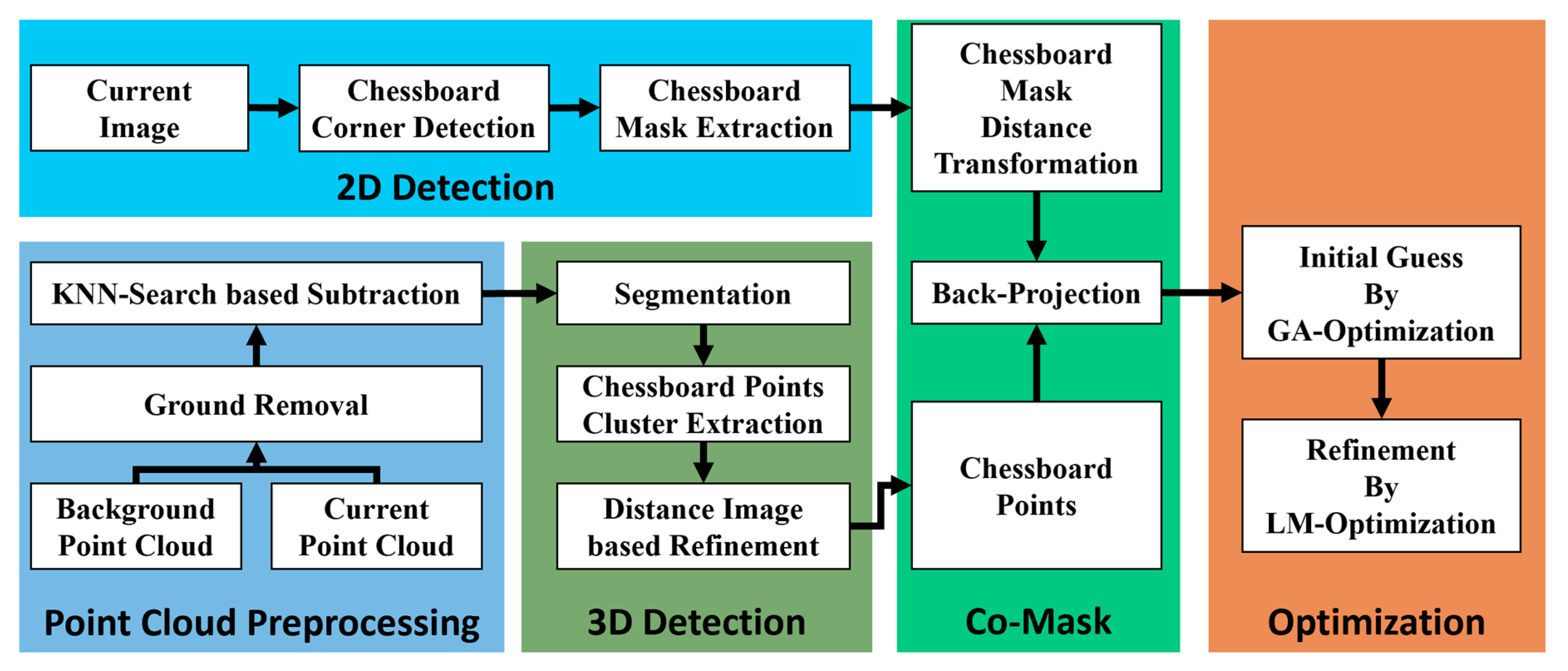
The main contributions of this article are shown in the following three points. First, we proposed an end-to-end framework aligning the correspondences between image mask regions and laser point cloud clusters. By constructing the distance transformation field of the checkerboard region, we directly back-projected the checkerboard point cloud to it, from which we built an energy function whose optimized result directly corresponded to the misalignment between the back-projected points and the region on the image plane. Secondly, a robust and efficient process for extracting checkerboard point cloud from complex and noisy background was put forward. In particular, we removed the background points by simple subtraction rather than designing many strategies and metrics to filter out interfering point clusters. Segmentation was applied to select the candidate point cluster including the checkerboard with spatial correlation, and the outliers on the plane were removed through binary morphological operation on the projected distance map. Finally, we carried out detailed simulated and realistic experiments, comparing our method to the state of the art. Furthermore, we also carefully analyzed how the range noise, number of observations, checkerboard distribution of distance and orientation, and initial parameters affected the final estimated results. We organized our code into a practical MATLAB GUI based calibration tool and made it open-source on GitHub with the following URL: https://github.com/ccyinlu/multimodal_data_studio.

This article is organized as follows. The second part introduces related works on extrinsic calibration of the camera and LiDAR. The third part shows the system flow as a whole. The fourth illustrates the process of checkerboard extraction both in the image plane and laser point cloud in detail. The fifth explains the optimization process. The sixth describes the experiments. The final section draws a conclusion.

2. Related Works

Due to the great value of camera–LiDAR fusion, the research topic of accurate, robust, and convenient extrinsic calibration has attracted a lot of attention. As mentioned above, the utilization of heterogeneous data such as images and the laser point cloud for extrinsic calibration mainly depends on the corresponding features or correlation information. These two ideas can be roughly categorized using comparison strategies such as target-based vs. target-less based, deterministic vs. non-deterministic, and offline vs. online.

Researchers [9,10,11,12,13,14,15,16,17] have carefully designed different types of calibration target for extrinsic calibration. Ha [18,19] designed a checkerboard with triangular holes, based on which the 3D–3D corresponding points were found. Dhall et al. [20] extracted the 3D position of the markers from the camera and LiDAR by pasting the arcuo mark on the plane board through human interaction and certain post-progress refinement, thus forming a set of 3D–3D correspondences for estimation. Geiger et al. [21] proposed an automatic method with one single shot of multiple checkerboards. This approach recovered the 3D structure from the process of camera-to-camera calibration. Then, camera–LiDAR calibration was performed under the constraints that planes of the checkerboards recovered from the images should coincide with the planes detected from the LiDAR data. As the checkerboard detection from the LiDAR point cloud is based on the random seeds, the method is not stable; therefore, careful layout for the environment setup is needed. Hassanein [22] and Guindel et al. [23] recovered 3D point cloud by binocular data, and then extracted the vertices of the box from both the visual data and laser point cloud to obtain the 3D–3D point pairs for extrinsic calibration. It is indeed possible to directly estimate the relationship between the two coordinate systems by looking for the 3D–3D corresponding points, but in obtaining 3D position of the markers directly from the camera there is susceptibility to noise. Furthermore, the intrinsic parameters must be assumed as perfect. Thus, the 3D–3D based method is not sufficiently accurate. In addition, the corresponding pairs need to be associated with no error. This process is not robust enough and often requires manual intervention.

Other studies [24,25,26] focused on finding the corresponding 3D–3D geometric lines and surfaces, and designed a series of loss functions to perform the calibration. Zhang and Pless [27] first published work on a calibration for a system comprising 2D LiDAR and a monocular camera. They extrinsically calibrated the two sensors under the constraint that in the camera coordinate system, the scalar projection of a vector between the origin and a point on the plane onto the normal of the plane equals the distance between the origin and the plane. Other methods [28,29] improved the setting of the loss function. For example, the calibration module [29] in the AUTOWARE open source software packages builds the loss function based on the constraint that the vectors formed by projected 3D checkerboard center from the camera coordinate system and the checkerboard plane points in laser coordinate system should be perpendicular to its normal. Unnikrishnan [30] used similar criteria to construct an optimization equation and designed the LCCT toolkit. Pandey et al. [31] extended the method and applied it to the Ford Campus Dataset [32]. Li et al. [17] extracted the geometric line features in the laser point cloud. Zhou et al. [33] further extracted 3D geometric objects such as lines and planes of the checkerboard and proved that the external parameter estimation was not affected by the distance. In this paper, a good calibration result was obtained in the close range with only one observation. In fact, the accurate extraction of these 3D line and surface features from the camera coordinate system is worthy of further questioning. The realistic camera model is complicated, and the data are susceptible to noise. Therefore, the accuracy of 3D geometric features estimated just by the camera intrinsic parameters is very unstable and the realistic results are not satisfactory.

Seeking corresponding 3D–2D points for extrinsic calibration [25,34,35] is more robust than methods based on 3D–3D points. The authors of [36,37] used triangles or polygons with triangular features. By extracting the edges of the checkerboard in the laser point cloud, the 3D intersection points of the edges are estimated. 3D–2D corresponding points are formed with the estimated 3D vertices and 2D plane corners on the image plane. It is worth noting that the noise on the edge of the laser point cloud is relatively large, and the situation for low-cost LiDAR is more serious. It is difficult to guarantee the accuracy of the estimated 3D vertices through edge extraction. Lyu [35] manually adjusted the position of the checkerboard in the laser point cloud, so that the scan line could just scan to the vertex of the checkerboard so as to obtain 3D–2D point pairs. However, this enlarges the requirements for the observation and increases the overall time and complexity of the calibration process. Pusztai [38] used a box with three vertical sides as the calibration object. The 3D vertices of the box were estimated by extracting the edges, which formed 3D–2D point pairs. Wang [39] relied on the reflectivity information to extract the 3D coordinates of the checkerboard inner corner points from the laser point cloud and then formed 3D–2D point pairs. Like the above methods based on 3D–3D point pairs, these methods based on 3D–2D point pairs also need to obtain a clear correspondence relationship, which makes the final calibration accuracy unstable. In addition, the 3D–2D relationship association often fails to cope with complex environment and usually requires manual intervention.

In order to eliminate the limitation of calibration targets and enable online calibration through natural scenes, researchers have conducted many studies [40,41,42,43,44,45,46,47,48,49]. Some of these methods use the correlation between image color and LiDAR reflectivity [43,45,50,51], and some extract the edge [41,44] and line features [24,48] from visual data and the laser point cloud. These target-less methods are highly environment-dependent. Because the loss function cannot guarantee convexity in a large range, it requires relatively accurate initial parameters; otherwise it is easy to fall into local extreme. Thus, target-less calibration methods are generally used for online extrinsic parameter fine-tuning. There are some new explorations based on trajectory registration of visual–LiDAR odometry [52,53], SFM-based point cloud registration [40], or even deep learning technologies [54,55]. These methods are highly dependent on the environment and the result is affected by the accuracy of the visual or laser odometry. Generally, the accuracy of these method is not high enough and cannot be applied universally. Many other ideas [56,57,58] have been proposed to solve the extrinsic calibration problem for the camera and LiDAR. However, they were designed either for special imaging systems or applications with a dense point cloud.

Similar to the proposed method is the 3D–2D point pair-based method, although the authors of [39] used the checkerboard to generate deterministic correspondences, which may fail when the environment is more complex or the noise becomes larger. The approach by the author of [59] also showed similarity to our method to some extent. It estimates the extrinsic parameters based on contour registration from natural scenes. However, the natural sceneries that this method relies on have great uncertainty, and the accuracy and correlation of contour extraction from both image and laser point cloud cannot be guaranteed. The method in this paper uses the object-level 3D–2D correspondences between the checkerboard point cloud and region mask, and designs an effective method for extracting the checkerboard point cloud, which can ensure accuracy, stability, and noise resistance, and reduce dependence on the environment.

3. System Overview

An overview of the proposed method is illustrated in Figure 1. First, by extracting corner points of the checkerboard in the image and combining the inherent parameters, the mask of the checkerboard was estimated. Then, the Euclidean distance transformation of the mask was further generated. Secondly, the target point cloud and the static background had both ground points culled, and then the ground point-removed pairs were matched with nearest neighbor searching based on the KD tree to remove the background components from the target frame. For the remaining point cloud, segmentation based on depth continuity on range image was performed, and clusters with inner spatial correlations were separated. RANSAC-based plane extraction was executed on each cluster, and the corresponding significance scores indicating plane saliency were given. The cluster with the highest score was regarded as the final checkerboard point cloud candidate. A distance map of the candidate was then generated according to the extracted plane equation. Then, we binarized the distance map and deleted discrete small connected areas to eliminate outliers on the plane that did not belong to the checkerboard. After obtaining the 2D mask distance transformation and checkerboard point cloud, we constructed the energy loss function by back-projection from the laser point cloud to the distance transformation field, and established the correspondence between the 3D point sets and the 2D area. Finally, the genetic algorithm was applied to obtain a coarse estimation of extrinsic parameters that satisfied the projection of the 3D point cloud to the image plane area. The optimal result was further refined by the LM method.

4. Automatic Checkerboard Detection

In this paper, the checkerboard mask and distance transformation field were extracted, and were used to measure the mismatch between the 3D projection block and the mask area. By constructing correspondences between the 2D mask area and the 3D point cloud instead of 3D–2D point-level or geometric object-level correspondences, the system can effectively improve the noise resistance and robustness. Section 4.1 introduces how to obtain a 2D checkerboard distance transformation field. Section 4.2 explains in detail how to accurately extract the checkerboard 3D point cloud from a complex background.

4.1. 2D Checkerboard Distance Transform

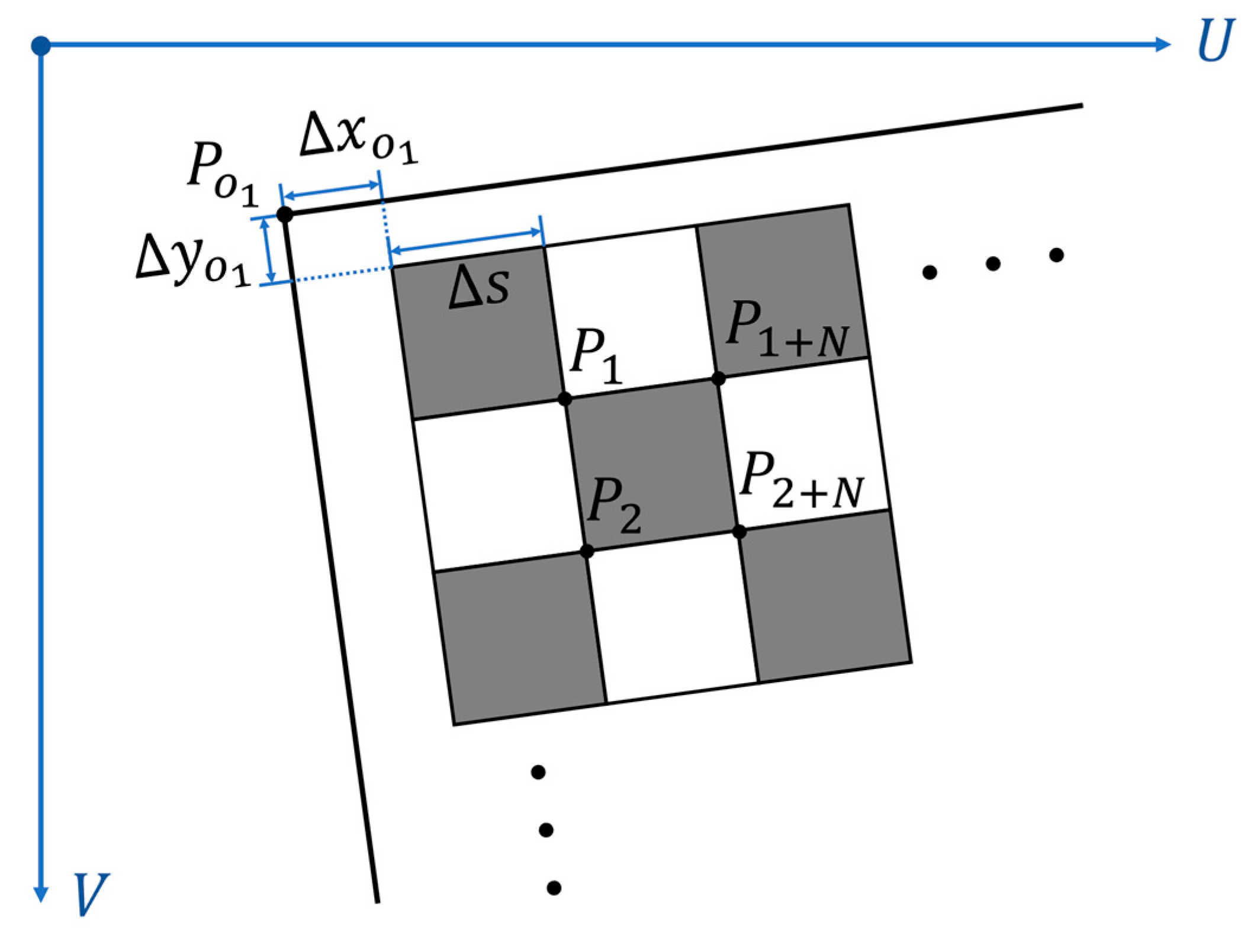
Methods [21,60] of checkerboard corner extraction from image have been developed relatively well. We used the method in [21] for this work. After the corners were obtained, the vertices of outer border could be calculated according to the $\left(u,v\right)$ coordinates of the surrounding inner corners and the inherent parameters of the checkerboard, as illustrated in Figure 2.

Points $\left\{P_1,P_2,P_{1+N},P_{2+N}\right\}$ represent the inner corners surrounding the top left outer vertex. $N$ represents the number of the corners along the $Y$ axis which is defined along the vertical direction, and $\mathsf{\Delta }s$ represents the side length of the square. Point $P_{o_1}$ represents the top left vertex of the outer boarder to be estimated. $\mathsf{\Delta }{x}_{o_1}$ represents the distance from the outer vertex to the nearest outer corner of the checkerboard pattern along the $X$ axis and $\mathsf{\Delta }{y}_{o_1}$ represents the distance along the $Y$ axis. The coordinate of the top left vertex on the $uv$ image plane can be calculated by Equation (1) without distortion considered.

$$U{V}_{P_{o_1}}=\frac{U{V}_{P_1}-U{V}_{P_{1+N}}}{\mathsf{\Delta }s}\left(\mathsf{\Delta }s+\mathsf{\Delta }{x}_{o_1}\right)+\frac{U{V}_{P_1}-U{V}_{P_2}}{\mathsf{\Delta }s}\left(\mathsf{\Delta }s+\mathsf{\Delta }{y}_{o_1}\right)+U{V}_{P_1}$$

(1)

In Equation (1), $U{V}_{P_1}$, $U{V}_{P_{1+N}}$, $U{V}_{P_2}$, $U{V}_{P_{o_1}}$ represent the coordinates on the $uv$ image plane of points $P_1,P_{1+N},P_2,$ and $P_{o_1}$, respectively. When the checkerboard has no outer boarder, which means the checkerboard pattern full fills the plate, the coordinate of the top left vertex can be simplified as Equation (2).

$$U{V}_{P_{o_1}}=2U{V}_{P_1}-U{V}_{P_{2+N}}$$

(2)

The establishment of the above equations needs to assume the shape of the checkerboard grid to be square and the distortion of the checkerboard image to be ignored. Experiments showed that the distortion was not obvious when the checkerboard was in the normal field of view. The accuracy of checkerboard corner extraction could achieve sub-pixel level, and the grid could basically meet the square constraint. Facts prove that linear extrapolation based on the above formula is feasible, and the error of checkerboard mask extraction introduced by ignoring distortion and corner extraction noise is basically negligible.

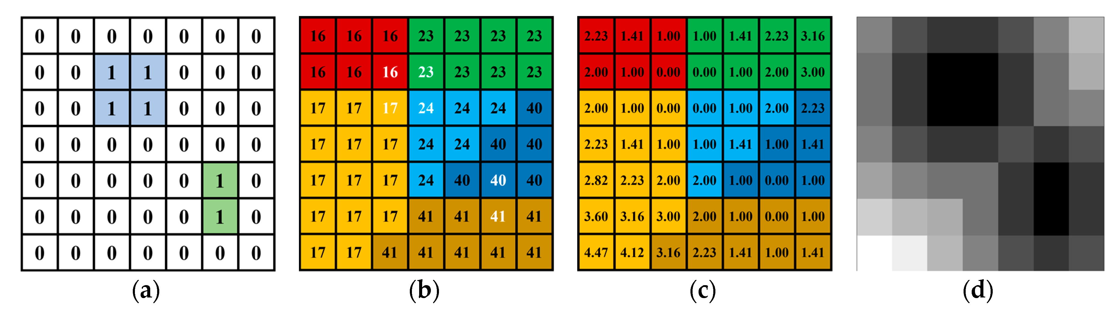
After obtaining the binary mask of the checkerboard, we performed Euclidean distance transformation, that is, the distance value of the pixel within the checkerboard mask was 0, and the greater the distance from the mask, the greater the distance value (Figure 3).

The Euclidean distance transformation field of the mask can be a novel way to measure the misalignment of the region, and has very good local convexity. When there is only one checkerboard mask on each image, it can ensure that all observations in the field of view of the camera have good convexity globally, which is very important for rapid convergence of the iteration.

4.2. Three-Dimensional Checkerboard Point Cloud Extraction

The method of using the checkerboard for extrinsic calibration of the camera and LiDAR generally needs to extract the checkerboard point cloud. Some of these methods [20,30] require manual interaction to assist in the selection of point cloud on the target. Others [37] require limiting and constraining the position of the target board. Some methods [39] are automated but design too many criteria based on the prior knowledge to filter out non-checkerboard points. All of these methods limit the experiment scene, increase the complexity of the work, and reduce the robustness of the system. The proposed method first filtered out the ground points in the target frame and the background to eliminate interference, and then differentially removed most complex background points from the target point cloud. The remaining point clusters were scored based on the flatness confidence, and the one with the highest score was identified as the final checkerboard candidate. A distance map was generated according to the most significant plane equation, and then the distance map was binarized and filtered out the outliers according to connectivity. Finally, we could obtain the accurate point cloud located on the checkerboard. The method of extracting the checkerboard point cloud in this paper has strong environmental adaptability and noise resistance, and can be easily extended to scenes with multiple checkerboards.

Due to factors such as the vibration of the vehicle platform, the mechanical rotation of the LiDAR, and the noise of the laser point cloud, even when the vehicle platform is stationary, the point cloud for the target frame and the background cannot completely overlap. In order to filter out background point cloud as much as possible, we relaxed the hit recall threshold. The impact of this strategy let the checkerboard points closer to the ground be considered on the ground and then be filtered out. This destroyed the integrity of the checkerboard points, but it is worth noting that the completeness of the point cloud extraction had a significant impact on the final extrinsic estimation. Therefore, it is necessary to filter the ground points first to eliminate the interference.

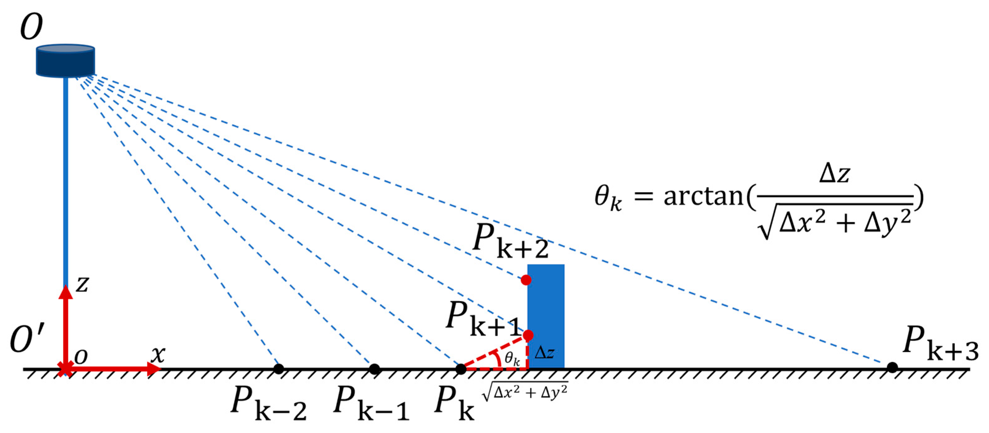
First, the irregular laser point cloud was ordered to generate a range image, and whether the point belonged to the ground was judged along each column of the range image. Figure 4 illustrates the process of ground point filtering. $P_{k-1},P_k,P_{k+1}$ represent the laser points located along the same column. The angle between the vector formed by two points on adjacent rows and the horizontal plane was used as an important basis for judging whether the point was located on the ground.

$$\{\begin{array}{c}{\mathbb{Q}}_g=\left\{P_k{|\mathsf{\Theta }}_k\le {\mathsf{\Theta }}_T|{\mathsf{\Theta }}_{k-1}\le {\mathsf{\Theta }}_T\right\}\\ {\mathsf{\Theta }}_k=arctan\left(\frac{z_{p_{k+1}}-z_{p_k}}{\sqrt{{\left(x_{p_{k+1}}-x_{p_k}\right)}^2+{\left(y_{p_{k+1}}-y_{p_k}\right)}^2}}\right)\end{array}$$

(3)

In Equation (3), ${\mathbb{Q}}_g$ represents the ground point set. ${\mathsf{\Theta }}_k$ represents the angle between the vector formed by point $P_k$ and $P_{k+1}$ and the horizontal plane. ${\mathsf{\Theta }}_T$ represents the threshold, which was set as 2° in this paper.

Figure 5 illustrates some results of the ground point filtering, and it can be seen that the ground points near the checkerboard were all eliminated.

In order to prevent the complex background from interfering with the checkerboard point cloud extraction, subtraction was applied to remove the background points. By constructing the KD tree of the background point cloud, the method reported in [61] was used to find the closest point of the background for each one of the target frames, which forms the nearest point pair. The point for which pair distance is greater than the threshold was considered as a new one and was filtered out.

In Equation (4), ${\mathbb{Q}}_{unmatched}$ represents the new point set compared to the static background. $p_t$ represents the point from the target frame. ${\widehat{p}}_b^t$ represents the nearest point to $p_t$, which was searched for from the background frame. $D_T$ represents the distance threshold. In this paper, it was set to 3 times the average distance of all the point pairs.

$$\{\begin{array}{c}{\mathbb{Q}}_{unmatched}=\left\{p_t|\Vert p_t-{\widehat{p}}_b^t\Vert \le D_T,p_t\in {\mathbb{Q}}_t,{\widehat{p}}_b^t\in {\mathbb{Q}}_b\right\}\\ D_T=3\ast std(\Vert p_t-{\widehat{p}}_b^t\Vert )\end{array}$$

(4)

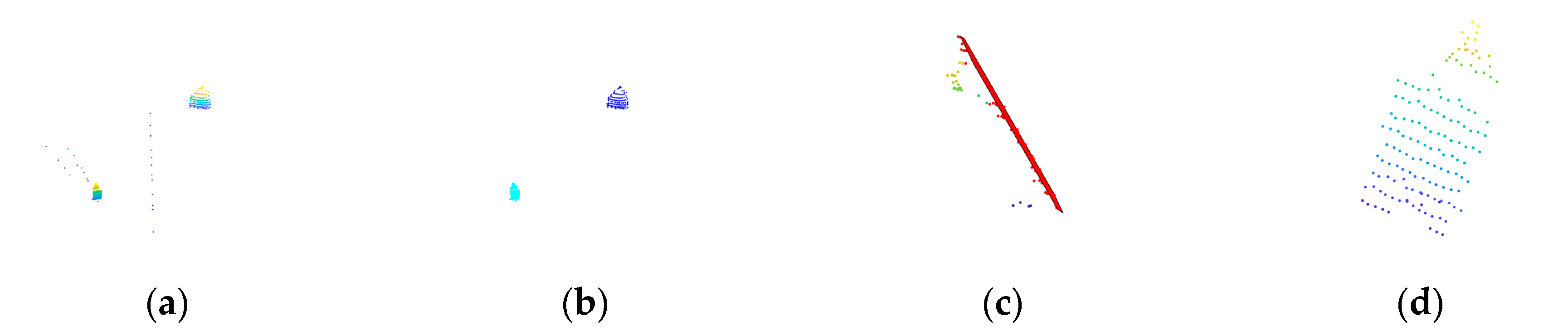
There could still be a large number of outliers in the newly added point cloud relative to the background, as the vehicle shows in Figure 5d. We needed to further cluster the point cloud with spatial correlation so that point clusters without the checkerboard were further removed. In this paper, the method reported in [62] was used to segment the serialized point cloud, and then the most significant plane equations of the clusters were estimated by the RANSAC [63] method; at the same time the corresponding interior was obtained.

$$scor{e}_{cluster}=\alpha \frac{N_{inliers}}{N_{inliers}+N_{outerliers}}+\beta \frac{N_{cluster}}{{\sum }_i{N}_{cluster}^i}$$

(5)

The significance score ($scor{e}_{cluster}$) for each remained cluster was calculated using Equation (5). $N_{inliers}$ represents the number of inliers. $N_{outerliers}$ represents the number of outliers. $N_{cluster}$ represents the number of all the points belong to the current cluster. $\sum _i{N}_{cluster}^i$ represents the number of the total points. $\alpha$ and $\beta$ represent the weight coefficient. In this paper, $\alpha$ was set to 0.3 and $\beta$ 0.7.

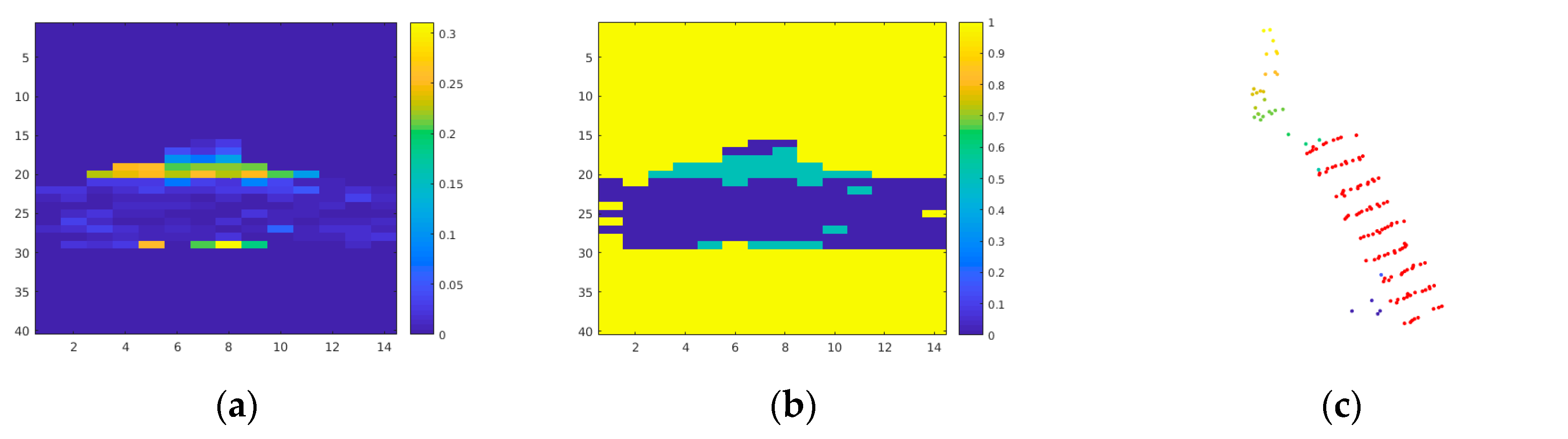
For fast data collection, we often hold the checkerboard by hand and move around in front of the camera. It can be seen from Figure 6c that the people’s head and some points on the body were on the same plane as the checkerboard. In fact, the points located on the holder and the support rod which are in contact with the checkerboard are always the outliers that satisfy the checkerboard plane equation but not in the checkerboard area. In order to extract complete checkerboard point cloud with noise, the flatness of the plane is often relaxed, which further increases the possibility of misjudging the aforementioned outliers into a checkerboard.

In this paper, the candidate cluster was projected to the most significant plane and the distance value of each point relative to the plane was calculated to generate a distance image after regularization. We then binarized the distance map and applied open operation on the binary map to eliminate discrete points and stickiness. The largest connected area was extracted from the processed binary map. Finally, the points corresponded to the biggest connected area were regarded as the final checkerboard points. Figure 7 illustrates the process of removing outliers of the points satisfy the plane equation.

5. Extrinsic Calibration Estimation

After obtaining distance transformation of the checkerboard mask on 2D image plane and the checkerboard 3D laser point cloud, the points were back-projected into the distance transformation field to construct an energy function. We took one single shot of the checkerboard with both the camera and LiDAR as one observation. After multiple observations, the energy function was accumulated. By minimizing this accumulated energy function, an accurate extrinsic transformation of the LiDAR relative to the camera was obtained.

$$p_i=\left[\begin{array}{c}u\\ v\end{array}\right]=\pi \left(\exp \left(\widehat{\xi }\right)\ast q_i\right), p_i\in P$$

(6)

We defined the current checkerboard points to set $Q$. For point $q_i={\left[\begin{array}{ccc}{x}_i& y_i& z_i\end{array}\right]}^T\in Q,$ we back-projected it to the image plane with Equation (6) to obtain the plane point $p_i$, in which $\pi (·)$ represents the transformation from 3D image space coordinate system to 2D image plane with distortion. That is to say, for the point in the 3D image coordinate system $P_c={\left[\begin{array}{ccc}{X}_c& Y_c& Z_c\end{array}\right]}^T$, we can use Equation (7).

$$\pi \left(P_c\right)=\left[\begin{array}{c}u\\ v\end{array}\right]=\left[\begin{array}{ccc}{f}_x& 0& c_x\\ 0& f_y& c_y\end{array}\right]g\left(P_c\right)$$

(7)

$$g\left(P_c\right)=\left[\begin{array}{c}{X}_{cg}\\ Y_{cg}\\ 1\end{array}\right]=\left[\begin{array}{c}\left(1+k_1{r}^2+k_2{r}^4+k_3{r}^6\right)\frac{X_c}{Z_c}+2p_1\frac{X_c}{Z_c}\frac{Y_c}{Z_c}+p_2\left(r^2+2{\left(\frac{X_c}{Z_c}\right)}^2\right)\\ \left(1+k_1{r}^2+k_2{r}^4+k_3{r}^6\right)\frac{Y_c}{Z_c}+p_1\left(r^2+2{\left(\frac{Y_c}{Z_c}\right)}^2\right)+2p_2\frac{X_c}{Z_c}\frac{Y_c}{Z_c}\\ 1\end{array}\right]$$

(8)

The specific expression of $g\left(P_c\right)$ in Equation (7) is illustrated in Equation (8). $g(·)$ indicates the transformation for distortion. $f_x$ and $f_y$ represent the focal length in pixel along the $X$ axis and $Y$ axis. $c_x$ and $c_y$ represent the coordinates of principal point in pixel along the $X$ axis and $Y$ axis. $k_1,k_2,k_3$ represent the radial distortion coefficients and $p_1,p_2$ represent the tangential distortion coefficients. $r^2$ in Equation (8) is expressed as: $r^2={\left(\frac{X_c}{Z_c}\right)}^2+{\left(\frac{Y_c}{Z_c}\right)}^2$.

The expression $\exp \left(\widehat{\xi }\right)$ in Equation (6) represents the coordinate transformation from the LiDAR system to the 3D camera system, which is an exponential mapping from $se\left(3\right)$ to $SE\left(3\right)$. $\widehat{\xi }$ represents a transformation in the space of $se\left(3\right)$ and it can be expressed by a rotation matrix and a translation vector in Equation (9). The relationship between $\exp \left(\widehat{\xi }\right)$ and Euler transformation is illustrated in Equation (10).

$$\widehat{\xi }=\left[\begin{array}{cc}{\phi }^{^}& \rho \\ 0^T& 1\end{array}\right]$$

(9)

$$\exp \left(\widehat{\xi }\right)=\left[\begin{array}{cc}R& t\\ 0^T& 1\end{array}\right]$$

(10)

In Equation (10), $R$ represents the rotation matrix from LiDAR coordinate system to 3D camera system and $t$ represents the translation vector.

The energy function based on distance transformation field is defined in Equation (11).

$${\xi }^{\ast }=arg\left(\underset{\xi }{\min }\left(\frac{1}{M}{\displaystyle \sum }_j^M(\frac{1}{N_j}{\displaystyle \sum }_i^{N_j}{w}_{ij}{e}_{DT}^j(\pi \left(\exp \left(\widehat{\xi }\right)\ast q_i\right)\right)\right)$$

(11)

In Equation (11), $M$ represents the number of observations. $N_j$ represents the number of points on the checkerboard for $jth$ observation. $e_{DT}^j$ represents the distance transformation of the checkerboard mask for the $jth$ observation. $w_{ij}$ represents the weight of $ith$ point for the $jth$ observation which is expressed as $\exp \left(-e_{DT}^{ij}\right)$, while $e_{DT}^{ij}$ represents the distance transformation value of the $ith$ back-projected point for $jth$ observation. Since the energy function has good convexity and can obtain the analytical Jacobian matrix, the LM method can quickly converge to the correct value.

The energy function in the field of view of the camera is convex, and the optimal value can be obtained by the gradient descent method. However, a large uniform penalty is imposed outside the imaging area, where the problem of gradient disappearance occurs. In order to converge without an initial estimate, the genetic algorithm was used to obtain roughly correct initial values before gradient-based optimization. For improved accuracy, we dynamically adjusted the weight of the checkerboard points during the optimization process. The strategy for adjusting the weight of the projection point is that the greater the distance from the projection of the laser point cloud to the mask, the smaller the weight. The pseudo code flow chart is shown in Algorithm 1.

Algorithm 1 Co-Mask LiDAR Camera Calibration
Input: Checkerboard mask distance transformation $\left\{e_{DT}\right\}$, Checkerboard 3D points $\{\mathbb{Q}\}$ Output: Extrinsic parameters $se\left(3\right), \xi$ from LiDAR to Camera
1.	${\xi }_{init}$ = ${\mathbf{0}}^{\mathit{T}}$; GA_opti = true; LM_opti = False; $\left\{W\right\}$ = {$\mathbf{1}$}; $e$ = 0; iter = 0; ${\epsilon }_e^{GA}$ = 10;
2.	while iter > iterMax || ${\xi }_{delta}$ < ${\epsilon }_{ \xi }$
3.	for j = 1:length($\{\mathbb{Q}\}$)
4.	${\mathbb{Q}}_j$ = ${\{\mathbb{Q}\}}_j$; $e_{DT}{}_j$ = ${\left\{e_{DT}\right\}}_j$; $e_j$ = 0;
5.	for © = 1: getNumPoints (${\mathbb{Q}}_j$)
6.	$e_j^i=w_j^i{e}_{DT}{}_j^i(\pi (\exp ( \xi )\ast {\mathbb{Q}}_j^i)$; $e_j=e_j+e_j^i$;
7.	end for
8.	$e$ = $e$ + $e_j/\mathrm{getNumPoints}\left({\mathbb{Q}}_j\right)$;
9.	end for
10.	if GA_opti then;
11.	${\xi }_{next}$ = GA ($e,\xi ,$); // update $\xi$ based on GA optimization algorithm
12.	if $e<{\epsilon }_e^{GA}$ then;
13.	LM_opti = True; GA_opti = False;
14.	end if
15.	end if
16.	if LM_opti then;
17.	${\xi }_{next}$ = LM ($e,\xi ,$ jacobian ($e,\xi$)); // update $\xi$ based on LM algorithm
18.	$w_j^i$ = $\exp \left(-e_{DT}^{ij}\right)$;
19.	end if
20.	iter = iter + 1; ${\xi }_{delta}={\xi }_{next}$ − $\xi$; $\xi ={\xi }_{next}$;
21.	end while
22.	return$\xi$

6. Experiment

The experiment in this paper is composed of two parts: a simulated experiment based on the PreScan engine [64] and a realistic experiment on our driverless vehicle test platform. The results showed that the proposed method was superior that those in the state of the art in terms of accuracy, noise resistance, and robustness. Section 6.1 mainly introduces the setting of the simulated experiment and the corresponding parameters. In Section 6.2, we conduct a comparative experiment and show the results. In Section 6.3, we evaluate the performance of each comparison method on data sets with different noise levels. Section 6.4 introduces the actual experiment setup and details of the unmanned platform to be calibrated. Section 6.5 shows the performance of different compared methods on real data sets. In Section 6.6, we evaluate the performance of the proposed method under different conditions such as number of observations, distance, and orientation distribution of the checkerboard. Finally, Section 6.7 provides a brief analysis of the entire experiment.

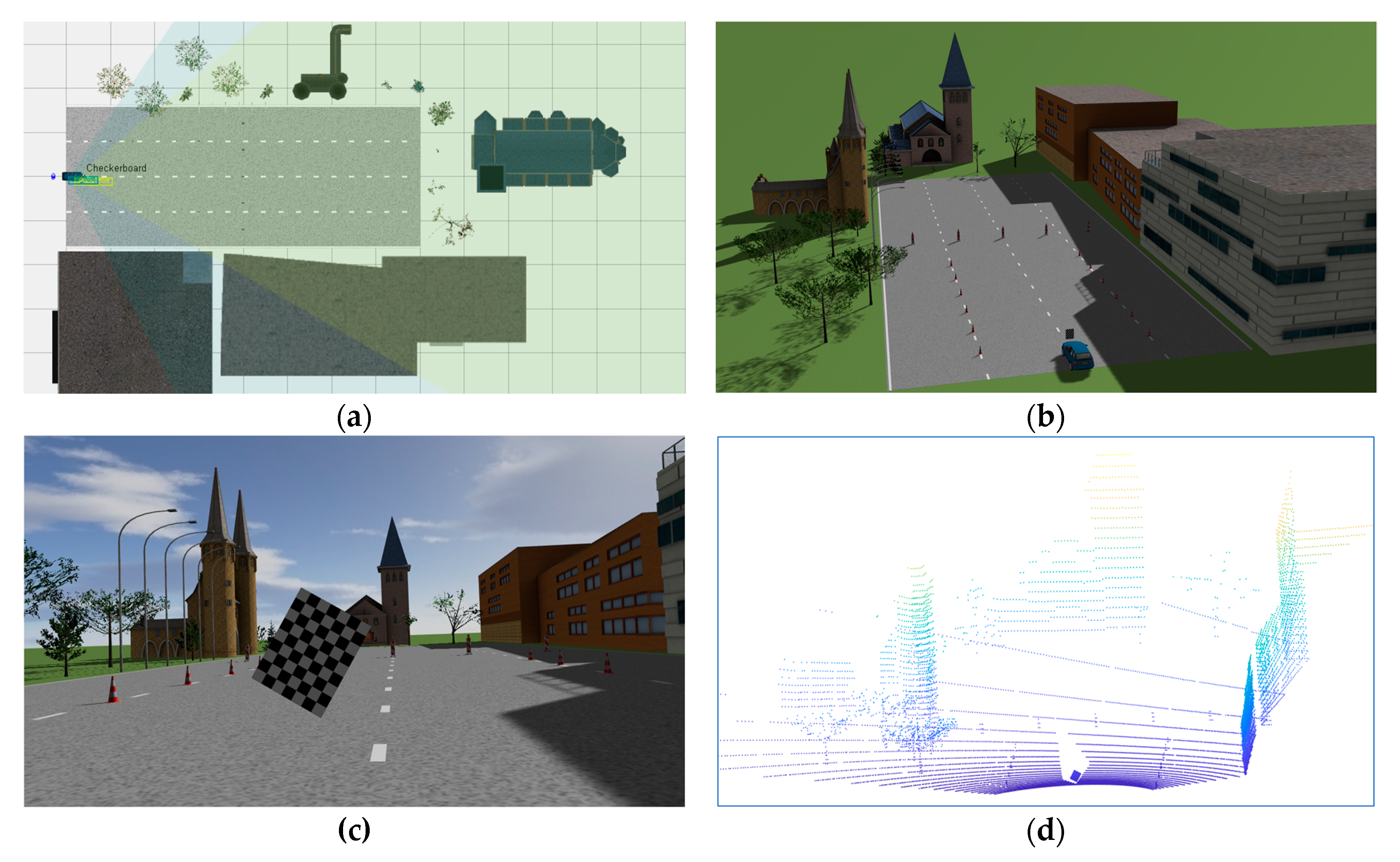
6.1. Simulated Experiment Setup

The PreScan simulator is a powerful software platform that assists industrial-grade autonomous driving design. It has rich scenes and models, which can quickly realize the construction of autonomous driving simulation scenarios and carry out model-based controller design (MIL), software-in-the-loop (SIL), and hardware-in-the-loop (HIL). Based on PreScan engine and MATLAB SIMULINK, we built a simple scenario for camera and LiDAR calibration, as shown in Figure 8.

The accuracy of the intrinsic parameters of the camera has a great influence on the extrinsic calibration. How to find an accurate intrinsic estimation is a hot topic that has been widely studied. We focused on extrinsic calibration of camera and LiDAR in this paper. The intrinsic parameters of the camera were estimated [65] in the following simulated and realistic experiments. Without losing generality, the camera in the simulated experiment had no distortion. All model positions in the PresScan engine were based on the car body coordinate system, which is generally defined as the right-handed system. In the simulation environment built in this paper, the 6 DOF extrinsic parameter $C_{SE3}$ of the camera relative to the car body coordinate system was $\left(2.0, 358.0, 5.0, 1.820,-0.300, 1.620\right)$, where the Euler angle is in degrees and the translation vector is in meters. The resolution of the camera model was 1280×720 pixels. The pixel was square with a side length of 4.08 um, and the focal length of the lens was set to 3.73 mm. The camera could be modeled as pinhole, based on which it could be quickly calculated that the horizontal angle of view of the camera was about 70° and the vertical angle of view was 43°.

The LiDAR used in the simulated experiment could obtain the reflectivity information of the point cloud. The 6 DOF extrinsic parameter $L_{SE3}$ of the LiDAR relative to the car was $\left(2.0, 3.0, 365.0, 0.500, 0.000, 2.400\right)$. The horizontal field of view of the LiDAR was 120° with resolution of 0.2°, and that of vertical field was 26° with resolution of 0.65°, forming 40 scan lines along the vertical direction. The reflectance value was normalized from 0 to 1.

6.2. Results of the Simulated Experiment

Gaussian noise was added to the perfect simulated data set. Since real image data is generally not very noisy and has little effect on mask extraction, we did not add noise to the image data. A real LiDAR point cloud can be spoiled with large noise in the distance and reflectivity due to factors such as changes in object reflectivity, vibration of rotating machinery, noise characteristics of electronic components, and TOF time measurement error of laser pulse echo. Noise has a significant impact on the checkerboard extraction and estimation of related geometric parameters. In this paper, Gaussian noise with a mean of 0 and a variance of 5 cm was added to the range information of the original noise-free laser point cloud data, and Gaussian noise with a mean of 0 and a variance of 0.1 was added to the reflectance value. We compared the methods of ILCC [39], AUTOWARE [29], and LCCT [30]. The specific results are shown in

Table 1. Results of the simulated experiments.

	6DOF-GT	Ours	ILCC	LCCT	AUTOWARE
$\mathsf{\Delta }Roll \left(deg\right)$	−85.3536	0.0370	0.2114	0.4933	0.7108
$\mathsf{\Delta }Pitch \left(deg\right)$	−0.4510	0.0347	−0.0896	−0.1192	0.1415
$\mathsf{\Delta }Yaw \left(deg\right)$	9.1579	−0.0181	−0.0206	0.1060	0.1392
$\mathsf{\Delta }X \left(cm\right)$	23.1805	0.0891	0.3260	3.6085	1.2533
$\mathsf{\Delta }Y \left(cm\right)$	137.6700	−0.7414	−1.1543	−2.0907	−0.0411
$\mathsf{\Delta }Z \left(cm\right)$	−70.1258	−0.2807	−2.0426	−7.6185	−5.7520
$\mathsf{\Delta }R$	-	0.0484	0.2209	0.5578	0.7652
$\mathsf{\Delta }T \left(cm\right)$	-	0.7978	2.3687	8.6853	5.8871

. The experimental results refer to the extrinsic parameter mean transformation from camera to LiDAR. In Table 1, $\mathsf{\Delta }Roll$, $\mathsf{\Delta }Pitch$, and $\mathsf{\Delta }Yaw$ are the errors between the estimated rotation angles around the $X$ axis, $Y$ axis, and $Z$ axis and the ground truth, respectively, in degrees. $\mathsf{\Delta }X$, $\mathsf{\Delta }Y,$ and $\mathsf{\Delta }Z$ represent the estimated translation. $\mathsf{\Delta }R$ is the modulus corresponding to the residual of the rotation matrix. $\mathsf{\Delta }T$ is the modulus of the corresponding translation vector.

It can be seen from Table 1 that the residuals of extrinsic parameters estimated by the method proposed and the ground truth were very close to 0. The column of 6DOF–GT represents the absolute extrinsic parameters of the ground truth while the others represent the delta value. Compared with other methods, the accuracy had a significant advantage.

After obtaining the extrinsic parameters between the camera and LiDAR, with the help of the intrinsic parameters, the laser point cloud could be projected onto the image 2D plane, thereby obtaining the one-by-one correspondence between the laser point cloud and the image plane coordinates. This process is called back-projection, for which the accuracy is relatively sensitive to the error of extrinsic parameters. Therefore, the precision of extrinsic calibration can be further intuitively judged by whether the back-projection is accurate. Partial results of the back-projection of the simulated experiment are illustrated in Figure 9. It can be seen from the Figure that although the noise with a variance of 5 cm was added to the distance, the extrinsic parameters estimated by the method proposed in this paper still had high accuracy, and the backward projection could obtain pixel-level matching accuracy.

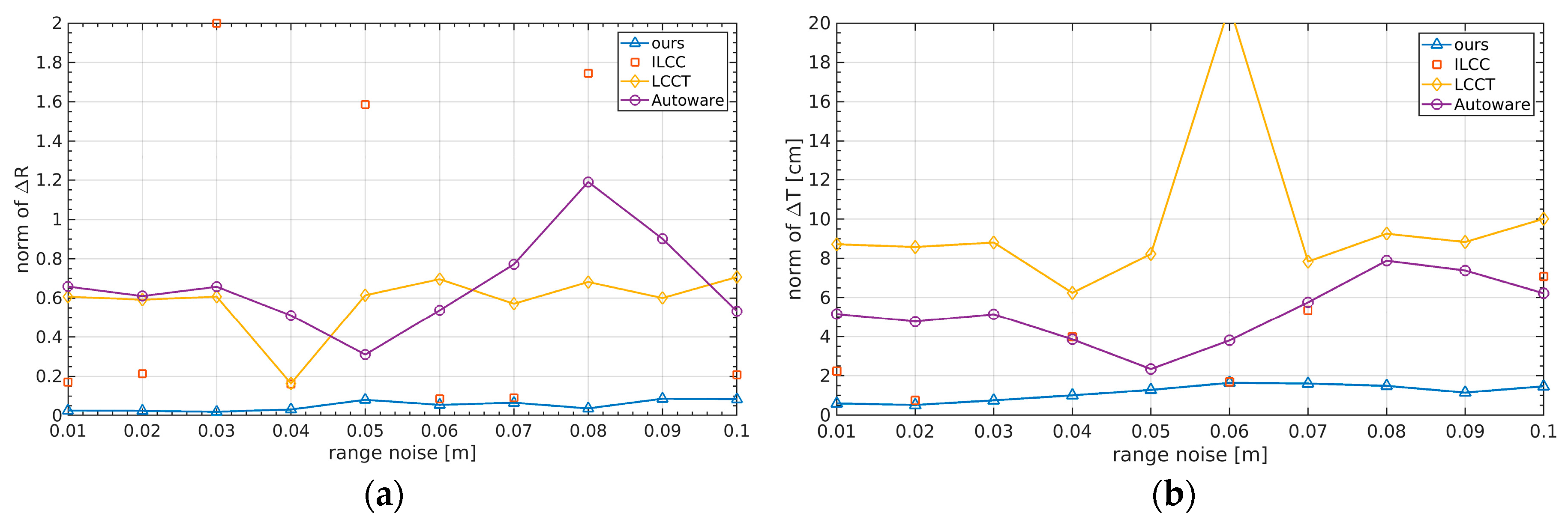
6.3. Simulated Results Vary with Noise

Realistic LiDAR data generally have non-negligible noise in range information. Relatively expensive LiDAR sensors such as Velodyne have high quality and the range noise generally does not exceed 2 cm. Relatively low-cost LiDAR sensors such as those of Hesai, Robosense, and Beike have greater noise, which greatly affects the calibration accuracy. In the method proposed in this paper, the detection of the checkerboard laser point cloud was robust, and could cope with various complex calibration environments. In the optimization process of extrinsic calibration, because there was no need to extract the geometric information of the checkerboard, instead the optimization strategy of aligning the checkerboard point cloud with the image mask was adopted, so it was naturally insensitive to noise. In the simulation part of this paper, a different level of noise was applied to the laser point cloud, and a comparison of different methods was carried out.

Simulated results under different noise levels are illustrated in Figure 10. The horizontal axis corresponds to the noise variance of range. As only the ILLC depends on intensity information, we did not add intensity noise to the simulated data. It can be seen that the proposed method had very high accuracy compared to the others. The LCCT and AUTOWARE methods need to rely on extracting the normal vector in the checkerboard point cloud, and construct the optimization equation through the constraints of the geometric relationship, which is easily contaminated by noise. The ILCC method needs to obtain the corresponding relationship between the checkerboard 3D–2D corner points to optimize the external parameters. Once the noise leads to partial extraction of checkboard points, the complete correspondence is destroyed, which greatly affects the optimization convergence direction or even causes convergence failure. It can be seen that when the data set was under certain noise levels, at times the ILCC method could not obtain correct results. When results were correct, the accuracy was not as good as in the method in this article.

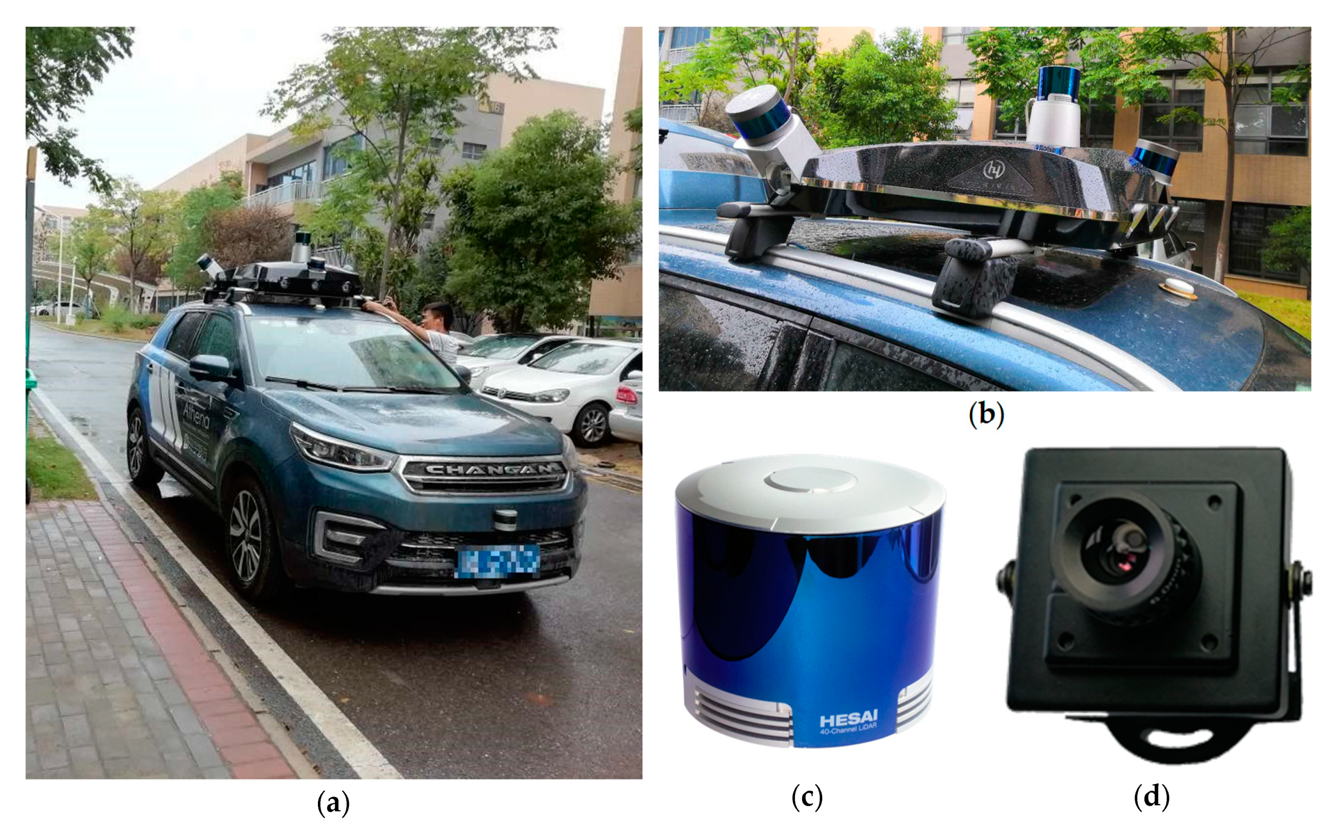
6.4. Realistic Experiment Setup

The real experiment in this paper was carried out on an unmanned vehicle platform. The calibration of the camera and LiDAR was mainly used to integrate visual data and laser point cloud for target detection and high-precision SLAM. The experimental equipment is shown in Figure 11.

Figure 11a shows an unmanned vehicle modified by a Changan SUV. Figure 11b shows a self-developed integrated sensor gantry which was equipped with a horizontal 360-degree lookout Hesai Pandar 40P LiDAR mainly used for the measurement of mid-range and long-range targets. The front, left, and right of the gantry were equipped with a 360-degree Robosense mechanical scanning 16-line LiDAR, which was used to detect and perceive targets near the vehicle. The platform was equipped with three groups of cameras in the forward direction, of which the front-middle and the front-left had a medium distance field of view with 6-mm focal length, forming binocular stereo vision that mainly perceived obstacle targets at short and medium distances. The front right camera had an 18-mm telephoto lens which was used to observe far-away targets. There was a 2.8-mm short-focus camera on the left and right sides to observe the obstacles near the vehicle. Compared with the benches of other teams, the sensor layout was more greatly dispersed. Although the field of view was increased, the sensors were more greatly dispersed, bringing certain challenges to accurate extrinsic calibration. Figure 11c shows the Pandar 40P from Hesai Technology Co., Ltd. The LiDAR was a mechanical scanner with a 360° horizontal field of view and vertical field of view up to 15° and down to 25°. It had 40 lines in the vertical direction, but the resolution was not uniform. Figure 11d shows a self-developed CMOS camera with high dynamic range equipped with a 6.8-mm lens. The horizontal resolution was set to 1280 pixels and the vertical resolution to 720 pixels.

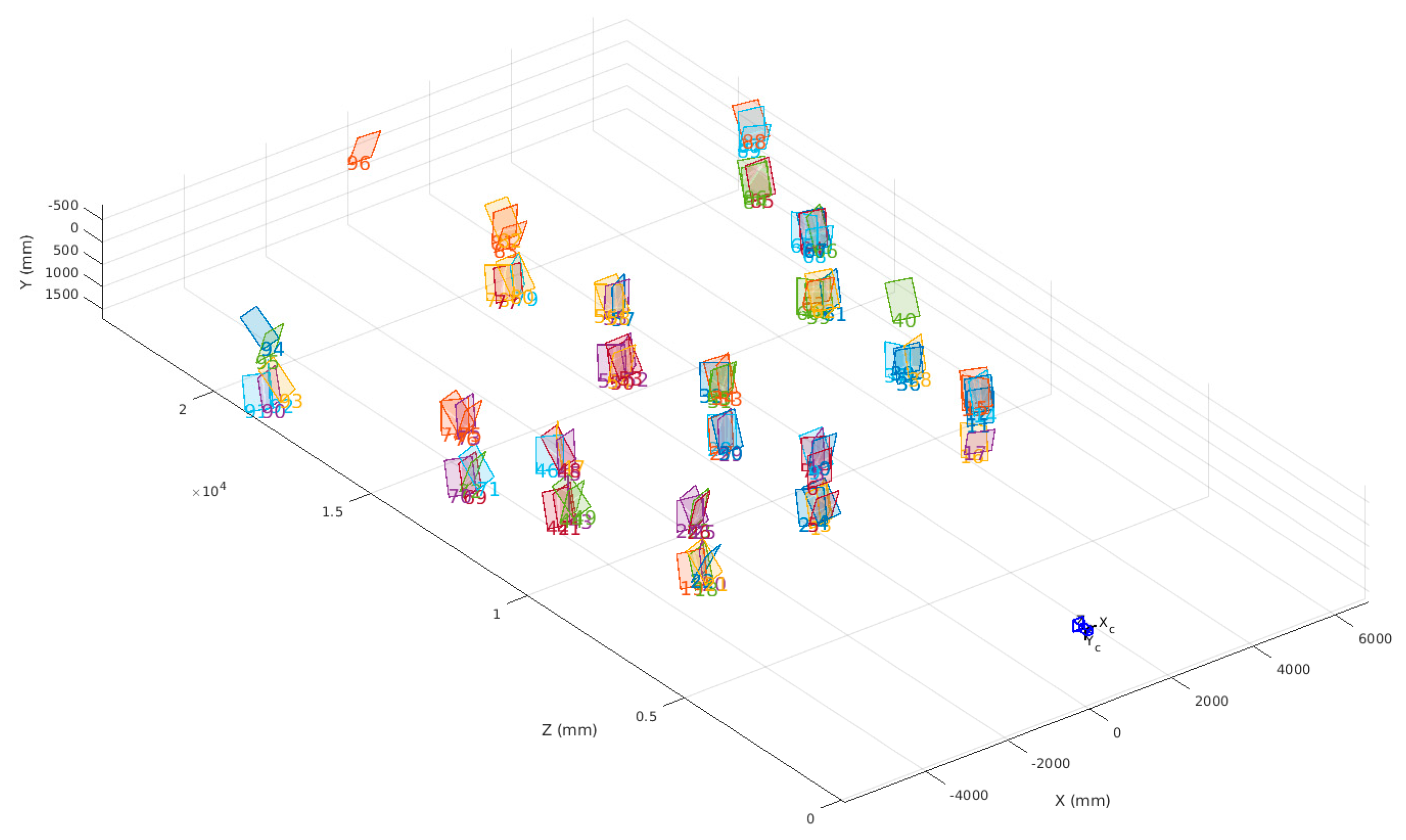
The observation data were collected by holding a checkerboard in the field of view of the camera and LiDAR. The calibration target had a checkerboard pattern printed on a rigid plastic board with 9 squares in the long direction and 7 squares in the short. Each checkerboard grid was a square with a side length of 108.5 mm. The size of the entire calibration board was 976.5×759.5 mm. The board had no white outer borders around the pattern. The realistic experiment collected a total of 100 pairs of LiDAR point clouds and images, one of which contained the reference data for the static environment. There were 3 pairs to be filtered out automatically due to low confidence. In the end there were 96 pairs of valid observations.

As shown in Figure 12, 96 effective observation samples were approximately evenly distributed in front of the vehicle in a fan shape with range from nearly 10 to 25 m. The observation sample at each position on the horizontal plane contained different postures and heights for the checkerboard. The checkerboard observation data of different distances, postures, and heights were collected to evaluate how the results varied as the checkerboard distribution changed.

6.5. Results of the Realistic Experiment

To evaluate the accuracy of the experiment, we needed to learn the ground truth. Even if we could obtain the installation position of the stand, due to the installation error and as the positional relationship between the sensor center and the mechanical casing cannot be accurately known, it would be impossible to obtain accurate real extrinsic parameters from direct measurement. Therefore, we qualitatively evaluated the experimental results by back-projection of the laser point cloud onto the image. Both the theory and the experiment showed that small changes in extrinsic parameters would result in projection errors that could be found visually, so the final accuracy and quality could be judged by visually projected residuals.

In this paper, all 96 observations were used for the experiment, and the initial parameters were not set due to the utilization of the genetic algorithm. The extrinsic parameters of the forward-facing camera relative to the center of the LiDAR were estimated, representing the transformation relationship from the point in the camera coordinate system to that of the LiDAR. The location of the Pandar40P LiDAR installed on the experimental platform was such that the LiDAR $X$ axis was roughly toward the left side of the vehicle, with the $Y$ axis pointing to the rear and the $Z$ axis vertically upward. We generally defined the camera coordinate system with the $Z$ axis pointing to the front of the camera, the $X$ axis perpendicular to the $Z$ axis points to the right of the camera, and the $Y$ axis down.

Table 2. Results of the realistic experiment.

$\mathsf{\Delta }\mathit{R}\mathit{o}\mathit{l}\mathit{l}/\mathit{d}\mathit{e}\mathit{g}$	$\mathsf{\Delta }\mathit{P}\mathit{i}\mathit{t}\mathit{c}\mathit{h}/\mathit{d}\mathit{e}\mathit{g}$	$\mathsf{\Delta }\mathit{Y}\mathit{a}\mathit{w}/\mathit{d}\mathit{e}\mathit{g}$	$\mathsf{\Delta }\mathit{X}/\mathit{c}\mathit{m}$	$\mathsf{\Delta }\mathit{Y}/\mathit{c}\mathit{m}$	$\mathsf{\Delta }\mathit{Z}/\mathit{c}\mathit{m}$
−90.2601	2.2371	179.4352	1.33	−28.54	34.13

shows the estimated extrinsic parameters which meet the relationship of the installation position of the sensor.

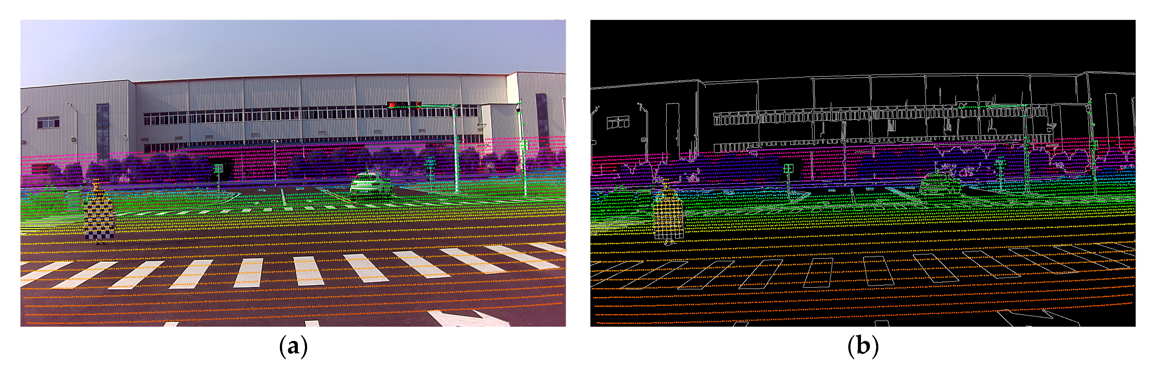
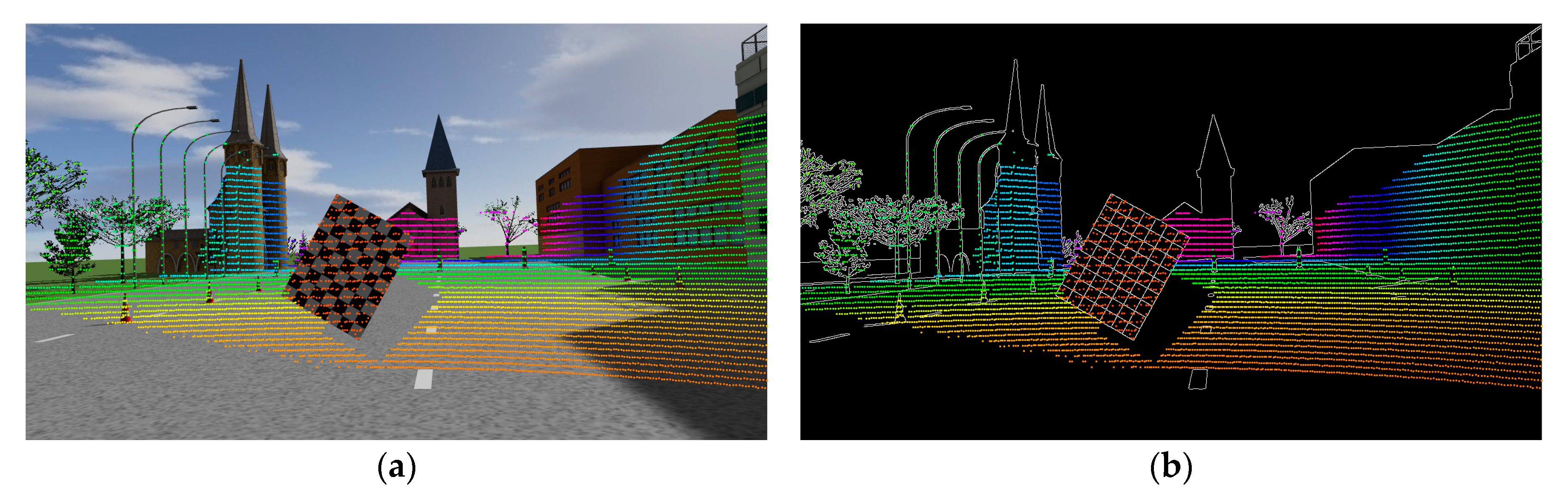
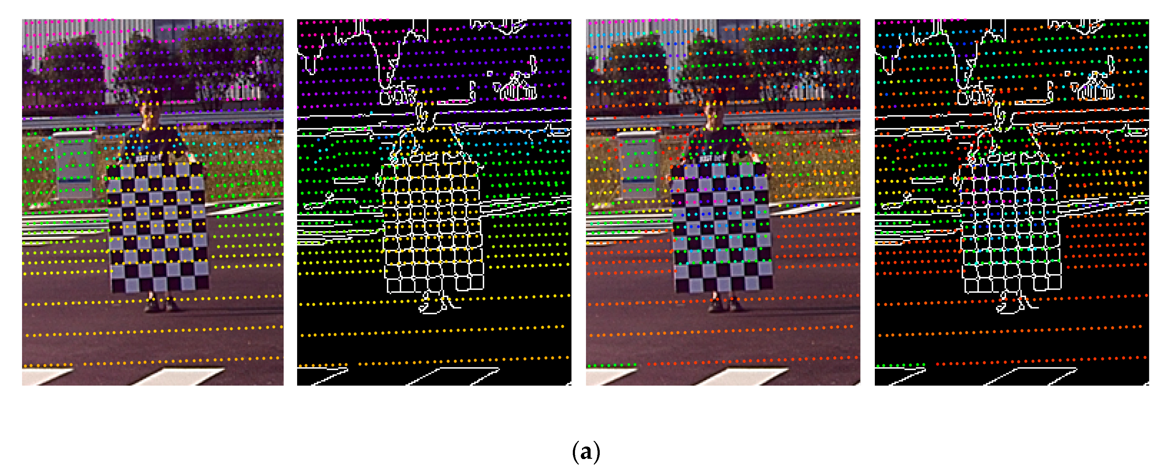
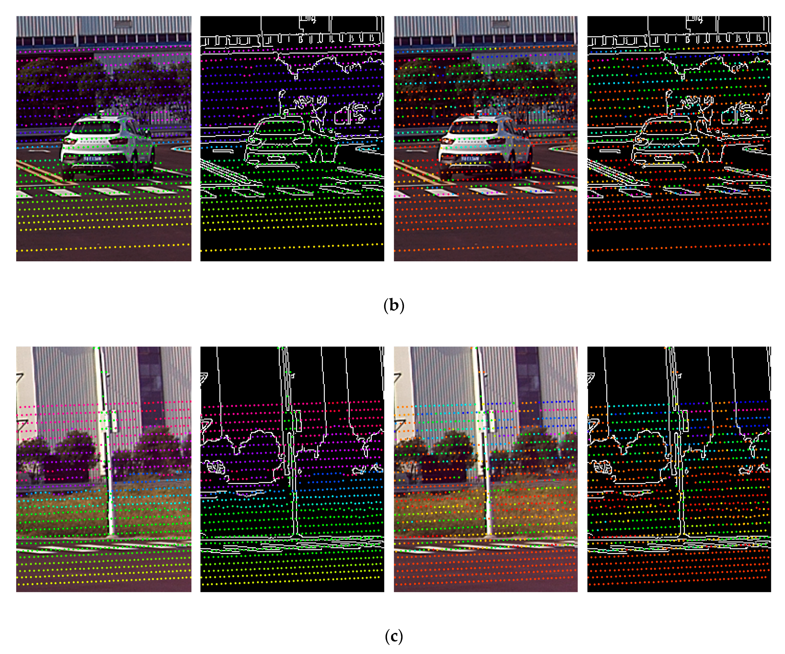
In Figure 13 the rendering of laser point cloud back-projected onto the image plane is illustrated. In order to accurately judge the projection accuracy visually, we used distance to render the projected points. At the same time, we also performed projection rendering on the edge map, which can more intuitively observe the alignment of the laser point cloud and the image edge.

It can be seen from Figure 13 that the extrinsic parameters estimated by the proposed method were accurate. Whether there were traffic signs, poles, checkerboards, or vehicles appearing in the scene, the 3D laser points were accurately projected onto the corresponding target in image. Even for trees and buildings at a distance of 50 m, as can be seen from Figure 13b, the discontinuity of the laser point cloud closely matched the edges of the image. It is worth noting that the point on the middle ring on the traffic sign which lay on the left of the vehicle was slightly shifted to the left, and the laser point cloud projection area on the sign to the right of the vehicle was larger than the corresponding area on the image. These were all due to the “halo” phenomenon of the LiDAR on the surface with strong reflectance, which belonged to the noise of the LiDAR point cloud itself.

Figure 14 shows the rendering effect of local zoomed patches. Figure 14a–c shows the zoom rendering effect of the three local sub-blocks. The columns ranging from left to right correspond to the distance rendering on the original image, distance rendering on the edge, reflectivity rendering on the original image, and reflectivity rendering on the edge, respectively.

Further details gave more evidence that the external parameters estimated had high accuracy. Further, we compared AUTOWARE [29] and LCCT [30], which are based on the corresponding normal, and the ILCC [39] method, which is based on 3D–2D checkerboard corners. As for the method based on the mutual information of reflectivity [45], the method based on the corresponding edge [41,44], and the method of extracting the corresponding points of 3D–2D based on SFM [40], the accuracy values cannot be compared with the target-based method, and rely heavily on the initial value. Thus, we did not compare these methods.

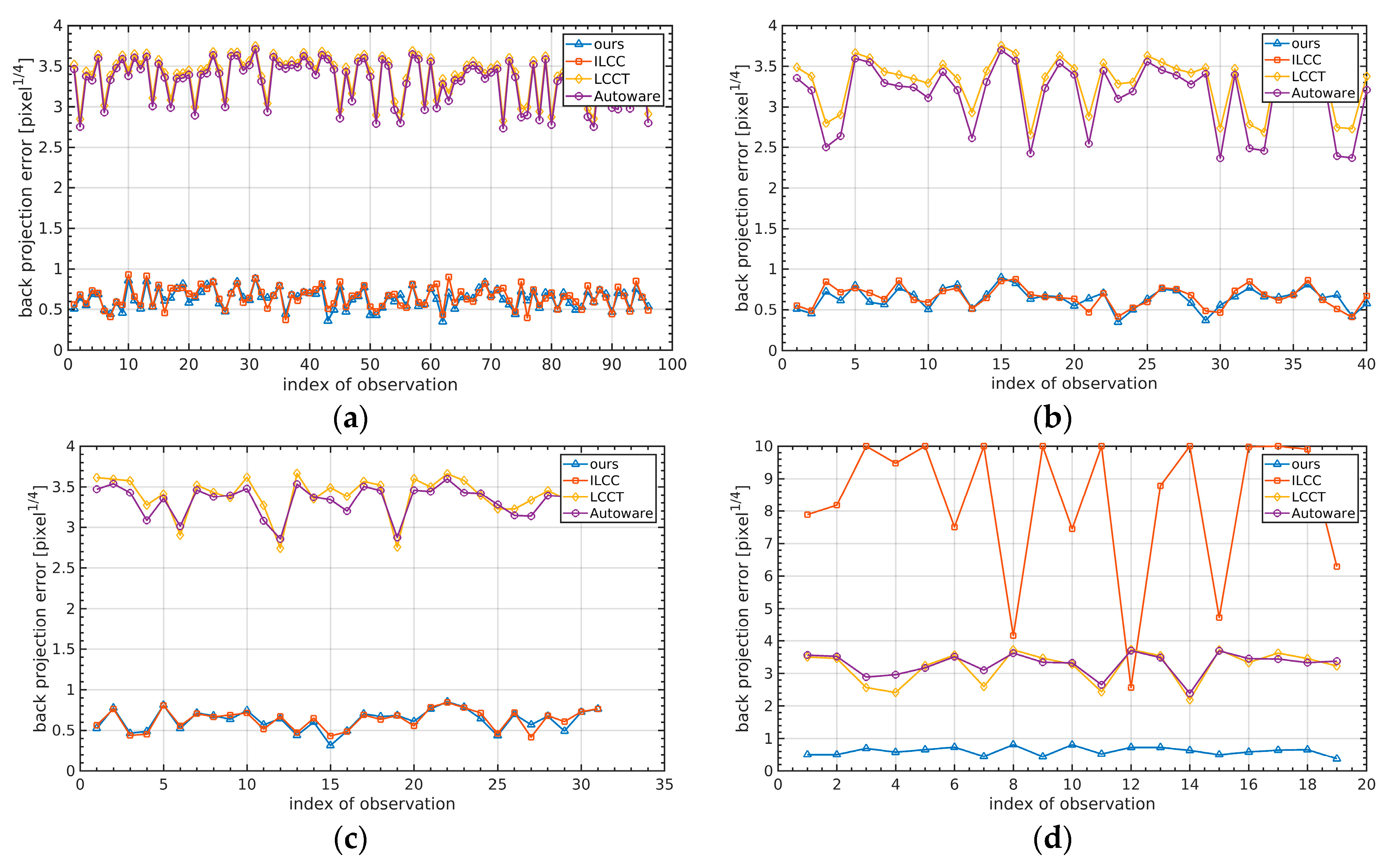
Figure 15 shows the back-projection errors of different comparative experiments, which represent the degree of mismatch between the projection block and the mask area after back-projection. AUTOWARE and LCCT rely too much on the geometric information of the checkerboard in the camera coordinate system, and the estimation of the extrinsic angle depends on the completeness of the orientation distribution for the observations. Therefore, the two methods had a large back-projection error in the real experiment of this paper. To make the visualization clearer, the vertical axis unit of the back-projection distance transformation residual curve was taken to be 1/4 of the power of the pixel. That is to say, the actual unit of the backward projection error was the pixel, and its true value was the fourth power of the value on the curve. It can be seen from Figure 15a that the method proposed in this paper and the ILCC method achieved an average back-projection error of about 0.2 pixels, which means the extrinsic calibration has high accuracy, while the error of AUTOWARE and LCCT was about 100 pixels. The ILCC method relies on the reflectance value to estimate the 3D–2D corresponding points. When the entire checkerboard points cannot be completely extracted, the ILCC method may converge to poor results. Therefore, we randomly selected 40%, 30%, and 20% of the total observations, and about 40, 31, and 19 observations, respectively, were tested. The experimental results are shown in Figure 15b–d. As can be seen, when the number of observations was reduced to 19, the ILCC method converged to the wrong value, making the re-projection error significantly increase. Compared with the ILCC method, our method does not rely heavily on observations and is extremely robust. Section 6.6 further elaborates the robustness of the proposed method.

6.6. Realistic Results Vary with Observations

Batch calibration work provides a frequent collection of calibration data sets. The lower the requirements of the calibration method for the number of observations, the distribution of the spatial distance, and the direction of the calibration board, the simpler the data collection work, and the more valuable the method is for commercial mass production. In this section, we discuss in detail how the results of our method changed when the number of observations, the spatial distance, and the orientation distribution varied. In addition, we also evaluated the convergence performance.

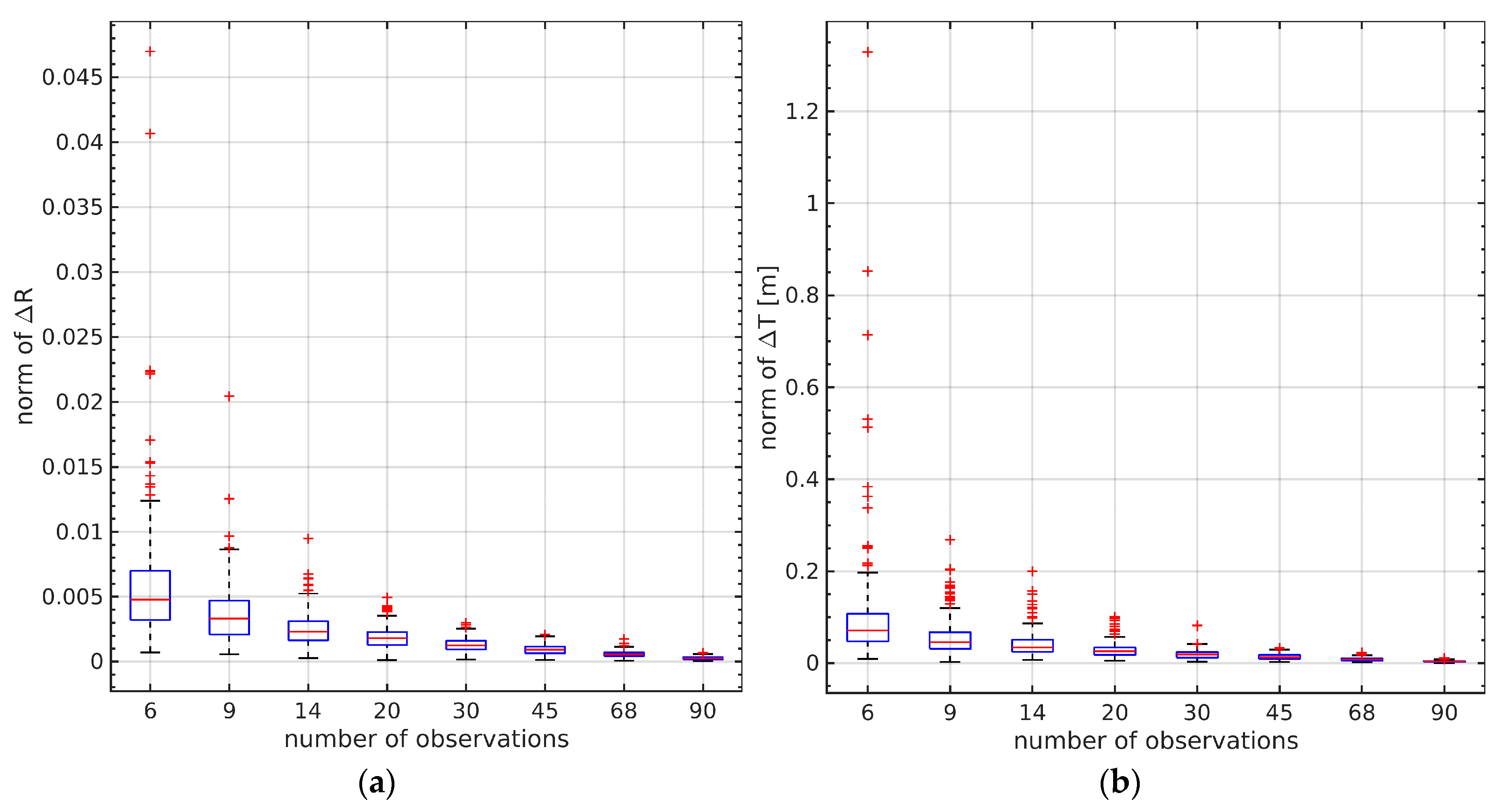
We randomly selected 6, 9, 14, 20, 30, 45, and 68 observations from the total of 96 for testing. Each experiment was randomly carried out 100 times. The results are shown in Figure 16. Section 6.5 showed that all 96 pairs of observations could be used to obtain near-true results. Since we could not obtain the true values of the extrinsic parameters on the current vehicle platform, we used the estimated ones by 96 observations instead. When the number of observations rose to 9, both the estimated rotation and translation were very close to the true value. With the further increase in the number of observations, the accuracy of the estimation results did not change significantly. This result shows that the proposed method does not have strict requirements with respect to the number of observations, and a small number can obtain accurate results, which undoubtedly brings hope to actual commercialization.

Further, we also studied the effect of the distance distribution of the checkerboard. Generally speaking, the noise of extrinsic parameters will significantly affect the projection results of distant targets. In order to control the calibration accuracy from far away, it is often necessary to collect samples at a distance, but the resolution of the images and point clouds of the distant targets is reduced and they are more susceptible to noise. Independence of spatial distribution of the calibration target is an important indicator to measure the quality of the calibration method. We divided 96 pairs of effective observations into 3 groups according to the spacing distances, which were not greater than 11 m, 11~17 m, and greater than 17 m. Each group randomly selected 15 pairs of observations for extrinsic calibration, and each group was randomly sampled 100 times. The results are shown in Figure 17.

It could be seen that when the number of samples in each group was set to 15, high accuracy could be obtained. Experimental data showed that the samples in the distance seemed to be more conducive to improving the overall accuracy, which is obvious. However, the use of nearby observations did not result in a large loss of accuracy.

We also evaluated the effect of different sample orientation distribution on accuracy. The angle between the checkerboard normal vector and the Z axis of the camera was distributed between 20° and 50°. The samples were divided into three groups according to the angles, which were less than 20°, between 20° and 35°, and greater than 35°. Each group randomly selected 15 pairs and repeated 100 times. The experimental results are shown in Figure 18. The checkerboard sample groups of different poses all reached a high estimation accuracy. Attitude error $\mathsf{\Delta }R$ averaged 0.002, while the translation error was below 4 cm. The experimental results showed that the calibration accuracy was not affected by the checkerboard posture, so we can make the checkerboard face the camera as much as possible to improve the detection confidence of the checkerboard.

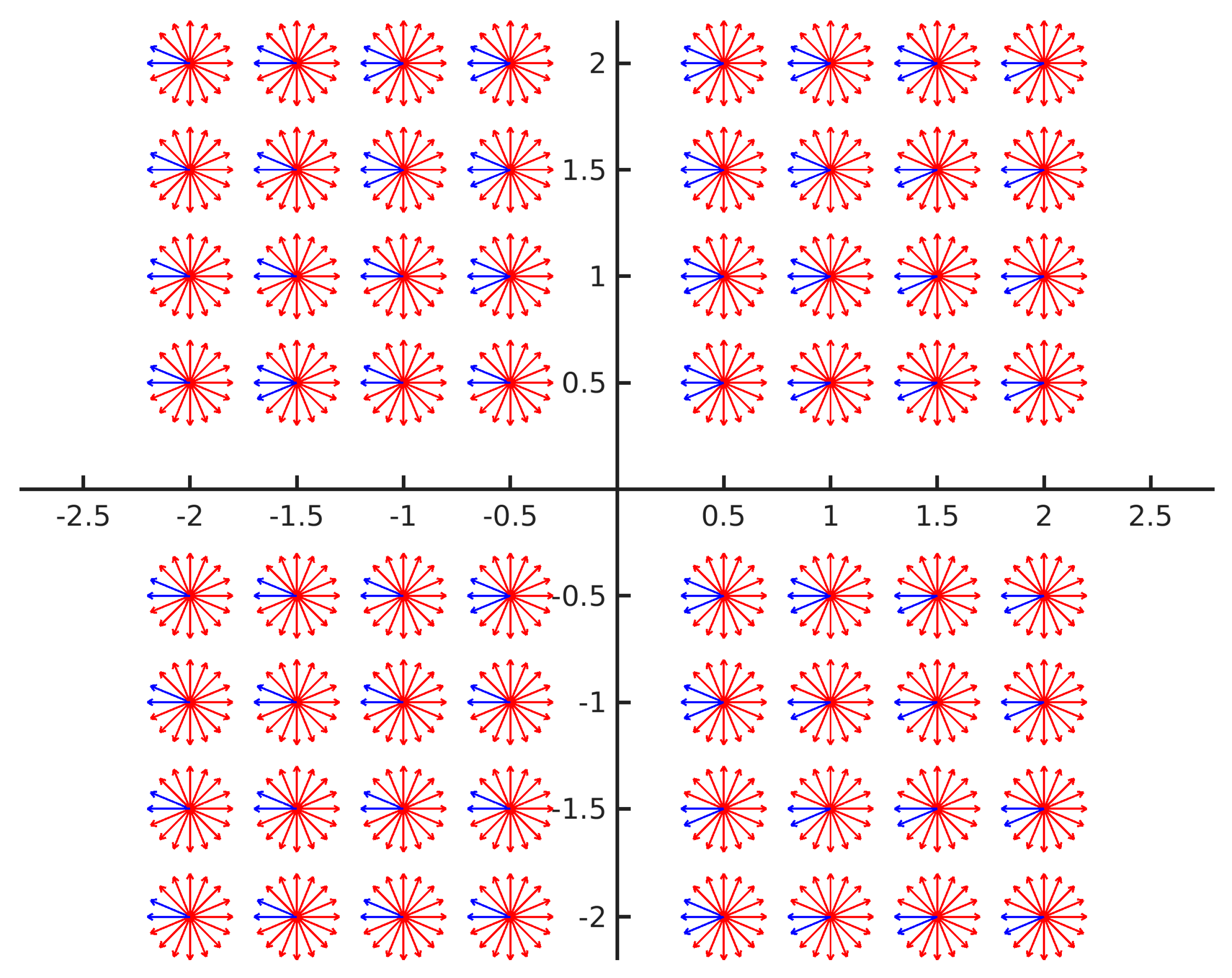
As mentioned above, the energy function constructed in this paper can converge within a relatively large range of initial values. Combined with the genetic algorithm, an initial value is estimated in advance so that the backward re-projection error is less than a certain threshold. The estimated external parameters can make the LiDAR point cloud roughly project into the camera field of view. The optimization process combining the genetic algorithm and LM method no longer depends on the initial value, and can converge to the true value from any position.

We conducted experiments to further verify the above conclusions. In order to make the visualization clearer and without loss of generality, we uniformly sampled the yaw, x, and y in the extrinsic parameter space, and kept the remaining parameters such as roll, pitch, and z at constant 0. The convergence of the energy function optimized only by the LM method under the above initial parameters was evaluated. When the LM method converged to the correct value, the average re-projection error was approximately 0.2 pixels. We consider that for optimization success the mean projection errors of the final convergence should not be greater than 0.5 pixels, and errors of more than 0.5 pixels are convergence failures.

As shown in Figure 19, the initial values at different positions can converge quite well. Compared with the position, the angle parameter has a greater influence on the convergence result. The disturbance of the initial parameter within 30° of the true value can converge to accurate results.

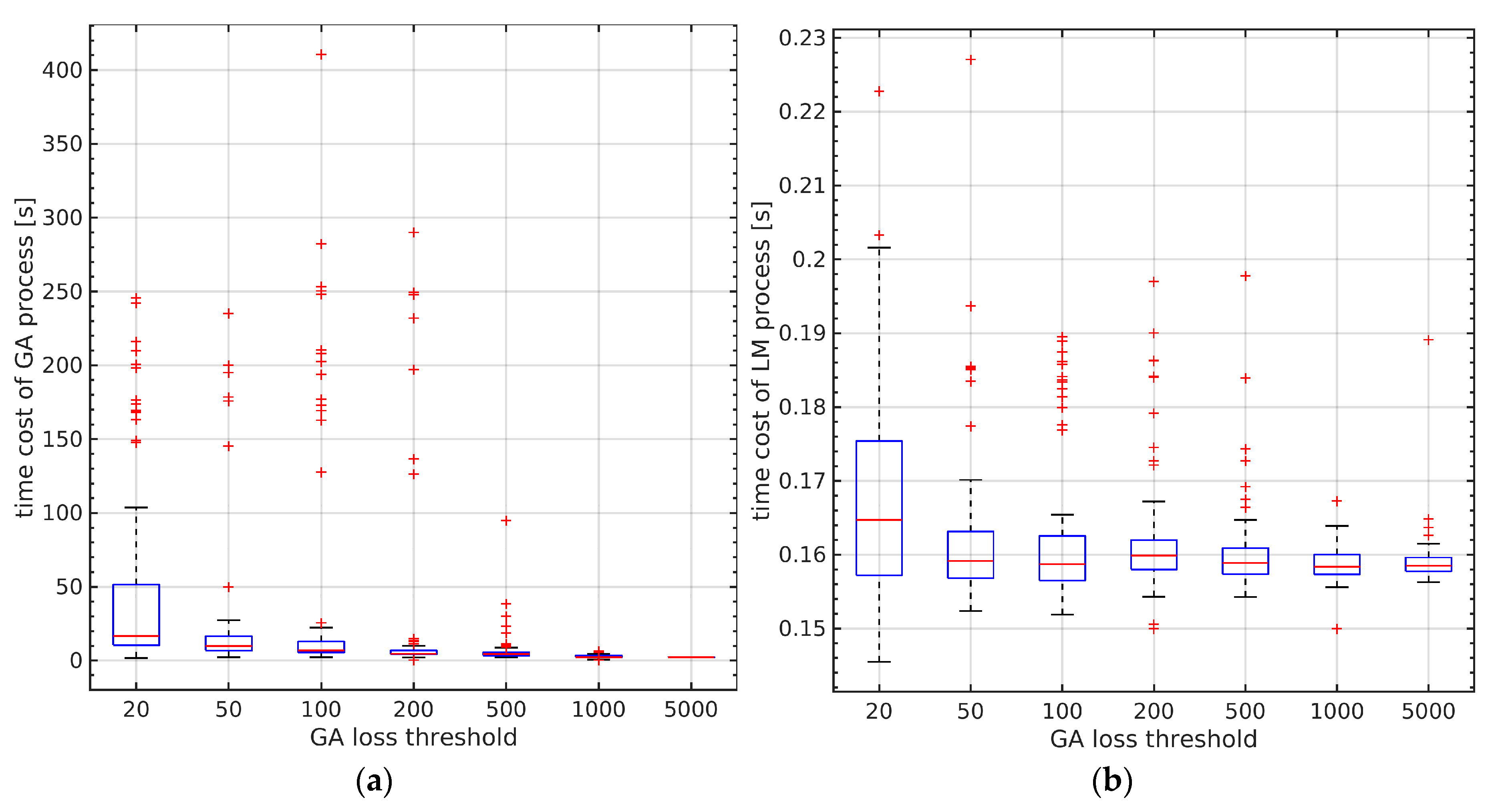
The optimization result combined with genetic algorithm is shown in Figure 20. We set the re-projection thresholds of GA to be 20, 50, 100, 200, 500, 1000, and 5000, respectively. Each group of experiments was carried out 100 times without initial values. All the experimental groups could converge successfully. We also evaluated the performance of the optimization. In Figure 20a, the time cost by different GA thresholds can be seen. The larger the GA threshold, the less time it took on average. Figure 20b shows that the optimization based on LM method converged very quickly and the time cost basically did not change with the initial parameters. The above results show that the loss function proposed in this paper has good convergence, and the optimization strategy combined with genetic algorithm can converge to the true value in a short time without initial parameters.

6.7. Analysis and Discussion

• Intrinsic parameters of the camera: If the checkerboard layout is not good enough or the real camera model is more complicated, using the method of traditional open-source OPENCV or MATLAB may not provide good results. A noisy intrinsic parameter will make it impossible to obtain accurate projection at different distances or views simultaneously; that is to say, the consistency of the extrinsic parameter is destroyed. As the method proposed is end-to-end, one observation is actually a control point to constrain the extrinsic parameters. We seek the minimization of the average projection error, so the projection residual for the position containing the control point is relatively small, while the position without the control point is relatively large. Observations can be grouped according to distance and view and extrinsic parameters can be estimated by each group separately to obtain smaller projection errors within the group.
• Checkerboard mask extraction: Frankly speaking, due to the distortion of the camera there is a certain systematic deviation in directly generating the checkerboard mask linearly from the corners of the distorted image. We have attempted super-pixel segmentation based on color features on the segmented checkerboard mask to make up for this. Experiments show that this operation helps only slightly and will even cause new errors due to the complexity of the background. For the ordinary camera lens, the distortion of the checkerboard is not very obvious, and the deviation caused by the slight distortion will be averaged out. Distortion has been taken into account when designing back-projection loss, and minor errors in the mask extraction process can be ignored.
• Checkerboard point cloud extraction: If the noise is large, the checkerboard is uneven, or the angle between the checkerboard normal and the Z axis of the camera is too large, it will result in the inability to extract a complete checkerboard point cloud. The method in this paper is a combination of multiple observations constraining to produce a minimum projection loss. Therefore, if the checkerboard point cloud is incomplete, it can still converge to the accurate results. Methods that are strictly based on 3D–2D corresponding points will fail.
• Calibration target: The proposed method does not need to obtain the deterministic 3D–2D corresponding points, but the relationship of the regions. Thus, the calibration board is not strictly required to be a checkerboard. For objects with different reflectance, the distance and its noise are different. The black and white squares on the checkerboard grid exacerbate this phenomenon. It is worth noting that if the checkerboard is too far away, it will make it impossible to detect all the corner points on the checkerboard, thereby invalidating the checkerboard mask area detection. If we want to seek high-quality extrinsic projection accuracy of distant targets, it is necessary to deploy control points in the distance. A white calibration board could be considered for use instead of the checkerboard. If the environment has a large texture contrast with the white calibration plate the area of the calibration plate can still be accurately extracted.
• Initial extrinsic parameter: In principle, it is possible to place multiple checkerboard calibration plates during one observation, which can significantly reduce the number of observations, but this will destroy the globally convex nature of the loss function with a need to further limit the initial parameters. Engineering applications can strike a balance between these two points. Since we do not use one-to-one corresponding 3D–3D or 3D–2D points, no prior knowledge is needed for the association relationship.

7. Conclusions

We propose a fully automated and robust method with high accuracy based on corresponding masks for extrinsic calibration between the camera and LiDAR. By seeking the object-level 3D–2D corresponding relationship, instead of looking for the 3D–2D corresponding corner points or 3D–3D pairs of points, lines, or planes, the new method not only lowers the requirements to data quality, but also insures the convergence stability. A series of simple but effective operations such as nearest-neighbor-based point cloud subtraction, spatial growth clustering, and segmentation on distance map based on mathematical morphology can quickly and robustly help to separate the checkerboard points from the complex background, and can eliminate the outliers adjacent to the checkerboard. By projecting the checkerboard points back to the distance transformation field, the energy loss function itself has good convexity, so it can converge to the global minimum under the condition of rough initial parameters. The two-step strategy utilizes the genetic algorithm to obtain a rough initial estimate, and further refinement by the LM method can solve the optimization problem without any prior knowledge, which enhances the robustness further.

Compared to typical 3D–2D point-based methods like ILCC and 3D–3D corresponding normal-based methods such as AUTOWARE and LCCT, both qualitative and quantitative experiments indicate that our method not only has a significant advantage in accuracy but also shows robustness to noise. Additionally, the proposed method is independent of distance and orientation distribution of the checkerboard and can achieve pixel-level accuracy with small number of observations. Based on the proposed method, we have developed a MATLAB GUI based tool for extrinsic calibration of the camera and LiDAR. The code is open-source on GitHub and the URL is https://github.com/ccyinlu/multimodal_data_studio.