Permeable Breakwaters Performance Modeling: A Comparative Study of Machine Learning Techniques

Abstract

The advantage of permeable breakwaters over more traditional types has attracted great interest in the behavior of these structures in the field of engineering. The main objective of this study is to apply 19 well-known machine learning regressors to derive the best model of innovative breakwater hydrodynamic behavior with reflection and transmission coefficients as the target parameters. A database of 360 laboratory tests on the low-scale breakwater is used to establish the model. The proposed models link the reflection and transmission coefficients to seven dimensionless parameters, including relative chamber width, relative rockfill height, relative chamber width in terms of wavelength, wave steepness, wave number multiplied by water depth, and relative wave height in terms of rockfill height. For the validation of the models, the cross-validation method was used for all models except the multilayer perceptron neural network (MLP) and genetic programming (GP) models. To validate the MLP and GP, the database is divided into three categories: training, validation, and testing. Furthermore, two explicit functional relationships are developed by utilizing the GP for each target. The exponential Gaussian process regression (GPR) model in predicting the reflection coefficient (R² = 0.95, OBJ function = 0.0273), and similarly, the exponential GPR model in predicting the transmission coefficient (R² = 0.98, OBJ function = 0.0267) showed the best performance and the highest correlation with the actual records and can further be used as a reference for engineers in practical work. Also, the sensitivity analysis of the proposed models determined that the relative height parameter of the rockfill material has the greatest contribution to the introduced breakwater behavior.

1. Introduction

Originally, ports were located naturally in a safe place away from natural hazards. However, with the increasing need for port space, engineers are always looking to build artificial structures named breakwaters in a cost-efficient manner with the least impact on the environment to eliminate wave energy and protect ports [1]. To build traditional types of breakwaters, such as rubble mound and the gravity type, a very high volume of material is required, which leads to an increase in the width of these breakwaters [2]. This volume of material reduces the naval area while changing the environment, ecology system, and landscaping [3]. Also, due to the disruption of the lateral drift process as well as water circulation, the construction of these structures causes severe erosion, heavy loading on nearby beaches, and a deterioration in the quality of water [2]. In addition, these breakwaters cause problems such as scour due to the high reflection of wave energy [1].

To solve the problems mentioned above, permeable breakwaters were introduced [4]. Although these types of breakwaters have a lower degree of protection compared to traditional breakwaters, their main advantage is to reduce the volume of materials and the structural problems of previous breakwaters. Also, these breakwaters cause the reduction of environmental problems and further increase the quality of water in ports [5]. 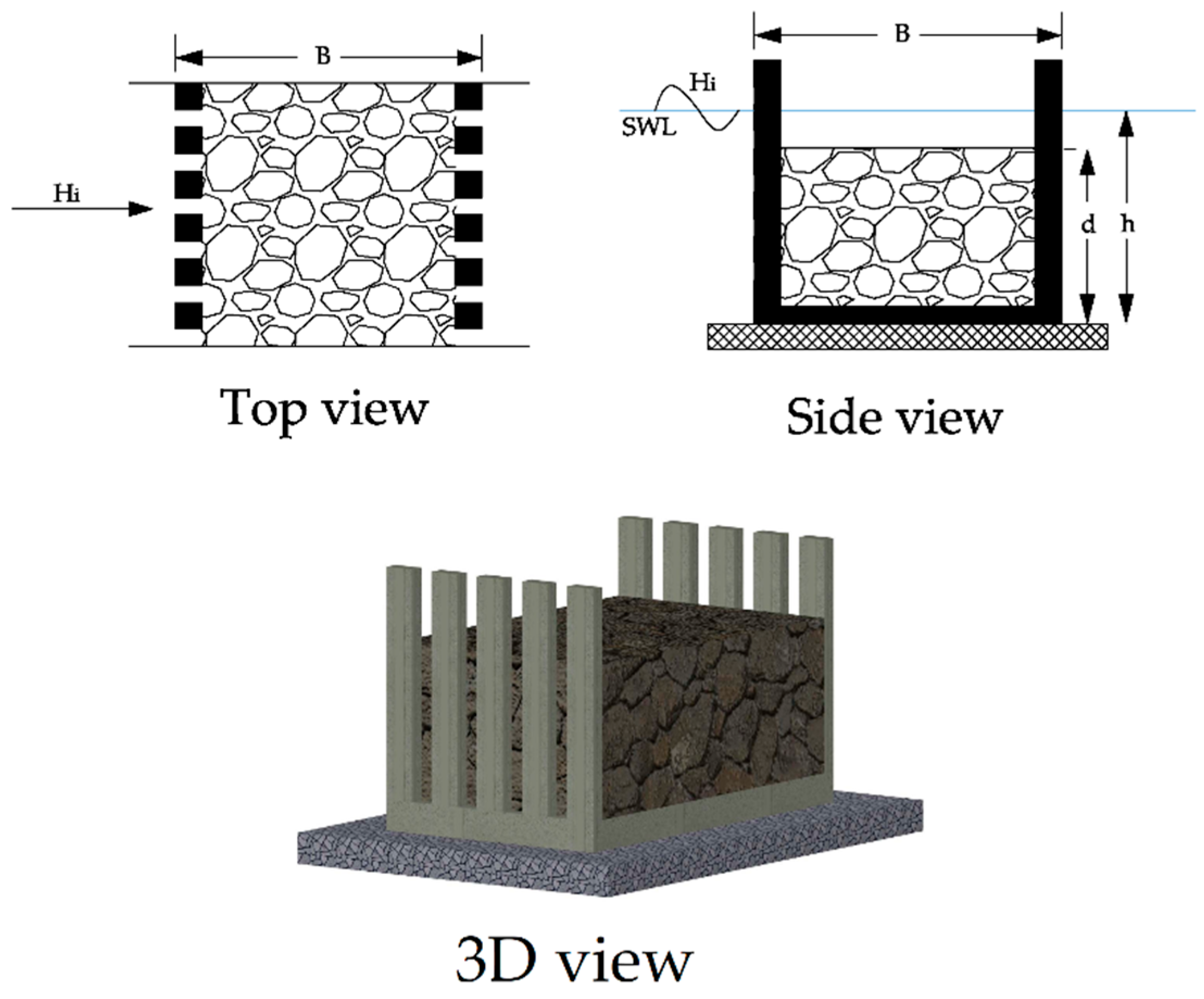The hydrodynamic performance of these breakwaters is measured based on wave reflection and transmission, which are expressed as coefficients of reflection and wave transmission [4]. In the following study, we have attempted to introduce an innovative hydrodynamic permeable breakwater behavior as a solution to improve the performance of the generation of this breakwater through lab experience. The introduced permeable breakwater is a two-layer vertical permeable type filled with high porosity rockfill materials (Figure 1). These materials change the flow patterns, and if used in the right way, could play a significant role in energy absorption and reduction of the transmission coefficient, which leads to the improvement of the level of protection and reliability of this type of breakwater, in addition to the advantages of the common permeable breakwater. This new type of permeable breakwater has many applications and can be used as a main or secondary breakwater and loading or unloading jetty. Also, it could be applied in different seabed conditions such as coastal slopes as well as various types of soil. In this study, the front permeable panel has a constant value of 50% permeability, and the rear panel permeability is variable.

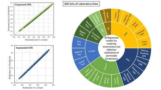
Machine learning methods have been widely used for the modeling of sophisticated engineering and sensing problems [6,7,8]. This study aims to model the hydrodynamic behavior of the breakwater with machine learning regressors (MLR). For comparison purposes, several widely used regression methods are employed, such as linear regression models, regression trees, support vector machine, Gaussian process regression models, ensembles of trees, and genetic programming. Based on the performance of the models, the best models will be selected, and knowledge will be extracted from optimal models.

Numerous studies have been conducted by the authors to investigate the hydraulic performance of these types of breakwaters, such as the total and semi-immersed, single, and double rows of vertical slotted pipes, and different kinds of wave screen breakwaters that consist of horizontal slots. In general, most of these studies have been conducted through hands-on experience in the lab. In addition, several analytical models have been used with the eigenfunction expansion of different wave theories [9,10,11,12,13]. These models alone are not capable of predicting the hydraulic performance of these breakwaters. In all models, the friction coefficient and added mass were obtained through the model calibration of the experimental results [9]. In 2013, Koraim et al. tabulated the specifications of the most important theoretical and laboratory studies in this field [4].

Due to the limitations of mathematical models, soft computing is widely used to solve a variety of classifications and prediction problems in science, medicine, and engineering [10]. In recent years, there has been increasing interest in using machine learning algorithms in marine engineering problems, especially those related to the modeling of breakwater behavior [11,12]. Elbisy (2015) used multiple additive regression trees (MART) and multi-layer perceptron neural networks (MLP) to quantify the regular wave runup on smooth slopes of perforated coastal structures constructed on sloping beaches. The results showed that the accuracy of the MART method is higher than the MLP methods [13]. In another study in 2016, Negm and Nassar presented the data for a new formula for wave reflection on smoothed, roughed, and perforated sloped seawalls using nonlinear regression. The results are consistent with previous studies; however, they remain limited in their application [14].

Yagci et al. (2005) modeled the damage rate of different breakwaters with three methods, such as artificial neural network, multilinear regression, and fuzzy logic model [15]. They argue that, unlike multilinear regression, which does not have satisfactory results, the other two methods would be able to interpolate data in the absence of abundant data. Recently, in another study, Pourzangbar et al. (2017), used two methods, namely support vector regression and model tree algorithm, to predict the maximum depth of scoring at breakwater toe from an average of 95 different experimental results. They recognized that the model obtained by the model tree algorithm was more accurate and showed better results than the experimental relationships [16]. Similarly, with the experimental data of Van Der Meer [17], Koç et al. (2017) studied the stability of rubble-mound breakwaters and proposed an explicit model by utilizing genetic programming. They showed GP models have better predictive performances than Van der Meer’s stability equations.

Previous studies have shown that each machine learning regressor has its strengths and weaknesses, and their performance depends on the characteristics of the subject under study [18]. Therefore, it is desirable to compare their performance in the modeling of introduced breakwater hydraulic behavior.

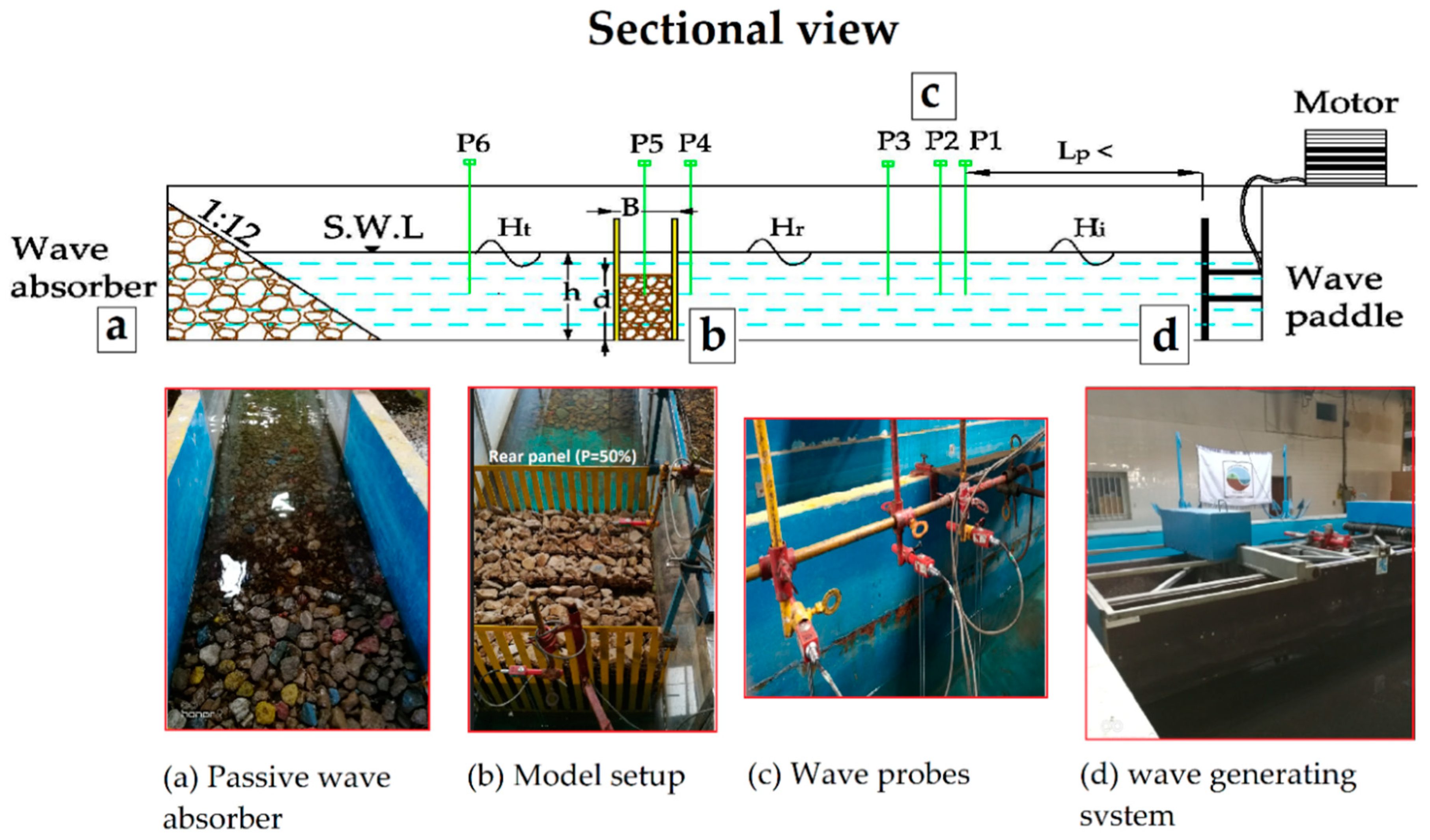
In this study, the hydrodynamic behavior of permeable breakwater under irregular waves has been studied. To fulfill this purpose, several machine learning regressors are employed to relate wave variables and breakwater parameters to the reflection and transmission properties of the structure by using 360 lab results.

2. Experimental Set-Up

The data used in this study are obtained from the experimental results on the physical model of the mentioned breakwater. The experiments are conducted in the laboratory of the Soil Conservation and Watershed Management Research Institute (SCWMRI) of the Ministry of Agriculture. Six wave probes are utilized to measure water elevation, which results in measuring reflection and transmission coefficients.

2.1. Physical Model Scale

To adjust the model scale, the equality of the Froude number that allows the correct reproduction of the gravitational and inertia forces of the flow was used, with the simulation scale of 1:25 which means, the length and time scales are 1:25 and 1:5 respectively. The range of model parameters and spectral wave variables have been listed in

Table 1. Ranges of principal experimental parameters.

Symbol	Definition	Range	Standard Deviation.
Lp	Spectrum wave length (cm)	0.85–5.15	1.16
Hs	Spectrum significant wave (cm)	2.91–14.20	3.21
d	Rockfill Height (cm)	30–56	9.63
B	Chamber width (cm)	16–80	22.63

.

2.2. Test Facility

The flume has 32.5 m long, 5.5 m wide, and 1-m depth that was equipped with a DHI wavemaker system. A pedal wavemaker is located at one end of the flume, and the other end of the flume contains a passive wave absorber in the shape of a porous beach, consisting of a 1:12 slope rock ramp to absorb energy and prevent reflection. The piston-generating pedal allows the generation of irregular waves perpendicular to the structure with proper steepness and different periods. Irregular waves have been used to reach the sea conditions, and the impact wave spectrum in experiments is the modified JONSWAP wave spectrum. Figure 2 shows the details of the experimental setup.

2.3. Physical Model Details

The introduced permeable breakwater is a two-layer vertical permeable breakwater where the chamber between the two panels is filled with high porosity rockfill materials (Figure 1). These materials modify the flow pattern and, if used correctly, can play a significant role in reducing energy absorption and the transmission coefficient. The front panel permeability is constant and set at 50%, while the rear panel permeability is set at 30% and 50% respectively.

3. Methodology

As mentioned, the study of wave information necessary to understand their hydrodynamic behavior [4]. These fundamental elements transmission and reflection of these structures provides key can be obtained through different methods, such as physical modeling and on-site investigation. However, implementing these methods is often cost-intensive and, in most cases, impossible [19]. Another approach is the use of mathematical models, however in practice, due to the complexity and nonlinearity of the problems, it remains challenging to obtain mathematical models. On the other hand, if such relationships exist, they should be validated with real data. Soft computing has been introduced to avoid the problems mentioned. The methods of machine learning used in this study are described below.

3.1. Linear Regression Model

Linear regression models have predictors that are linear in the model parameters, easily interpretable, and fast to perform. These properties make linear regression models the most popular models for initial use. However, the very limited shape of these models indicates that they often have poor prediction accuracy. After the application of a linear regression model, it is better to apply more flexible models, and thereafter compare the results.

3.2. Regression Tree

The classification and regression tree (CART) introduced by Breiman [20] is a kind of decision-tree algorithm that is made by recursive binary partitioning. CART is a method of creating a set of rules that ends in one class or value. CART can be used for classification and regression problems. If the target value is a categorical type, CART generates a classification tree, and when the response variable is continuous, it makes a regression tree. The result of using CART is a hierarchical binary tree that is created by dividing the subsets of the data, using all the predictor variables to generate two branches per node. This tree begins with the entire dataset. In each division, each predictor is evaluated to obtain the best cut-off point based on the degree of improvement or impurity. In the regression tree, the least-squares deviation impurity measure is used to divide the rules and integrity of fit criteria. This measurement is expressed by R(t) as follows [21]:

$$\mathrm{R}(\mathrm{t})=\frac{1}{{\mathrm{N}}_{\mathrm{w}}\left(\mathrm{t}\right)}{\displaystyle \sum _{\mathrm{i}\in \mathrm{t}}}{\mathrm{w}}_{\mathrm{i}}{\mathrm{f}}_{\mathrm{i}}{({\mathrm{y}}_{\mathrm{i}}-\mathrm{ȳ}(\mathrm{t}))}^2$$

(1)

$$\mathrm{ȳ}(\mathrm{t})=\frac{1}{{\mathrm{N}}_{\mathrm{w}}\left(\mathrm{t}\right)}{\displaystyle \sum _{\mathrm{i}\in \mathrm{t}}{\mathrm{w}}_{\mathrm{i}}{\mathrm{f}}_{\mathrm{i}}{\mathrm{y}}_{\mathrm{i}}}$$

(2)

$${\mathrm{N}}_{\mathrm{w}}\left(\mathrm{t}\right)={\displaystyle {\sum }_{\mathrm{i}\in \mathrm{t}}{\mathrm{w}}_{\mathrm{i}}{\mathrm{f}}_{\mathrm{i}}}$$

(3)

where N_w (t) is the weighted number of records in node t, W_i is the weighting field value for the record i (if any), f_i is the repeat field value (if any), У_i is the target field value, and $\mathrm{ȳ}\left(\mathrm{t}\right)$ is the mean value of the responding variable at node t.

The least-squares deviation (LDS) function for the division of s at node t is calculated as follows:

$$\mathrm{Q}(\mathrm{s},\mathrm{t})\mathrm{R}\left(\mathrm{t}\right)-{\mathrm{R}(\mathrm{t}}_{\mathrm{L}})-{\mathrm{R}(\mathrm{t}}_{\mathrm{R}})$$

(4)

where R(t_R) is the sum of the squares of the right child node, R(t_L) is the sum of the squares of the left child node, and the division of s is also chosen to maximize the value of Q(s,t).

3.3. Multilayer Perceptron Artificial Neural Network

McCulloch et al. established the neural network method in the early 1940s [22]. In general, a neural network is a predictive tool for constructing a mathematical model of an unknown system. One of the well-known or perhaps the most well-known of these models is the multilayer perceptron neural network, or MLP, which usually has a feed-forward architecture. The multilayer perceptron neural networks is often trained via the back-propagation algorithm.

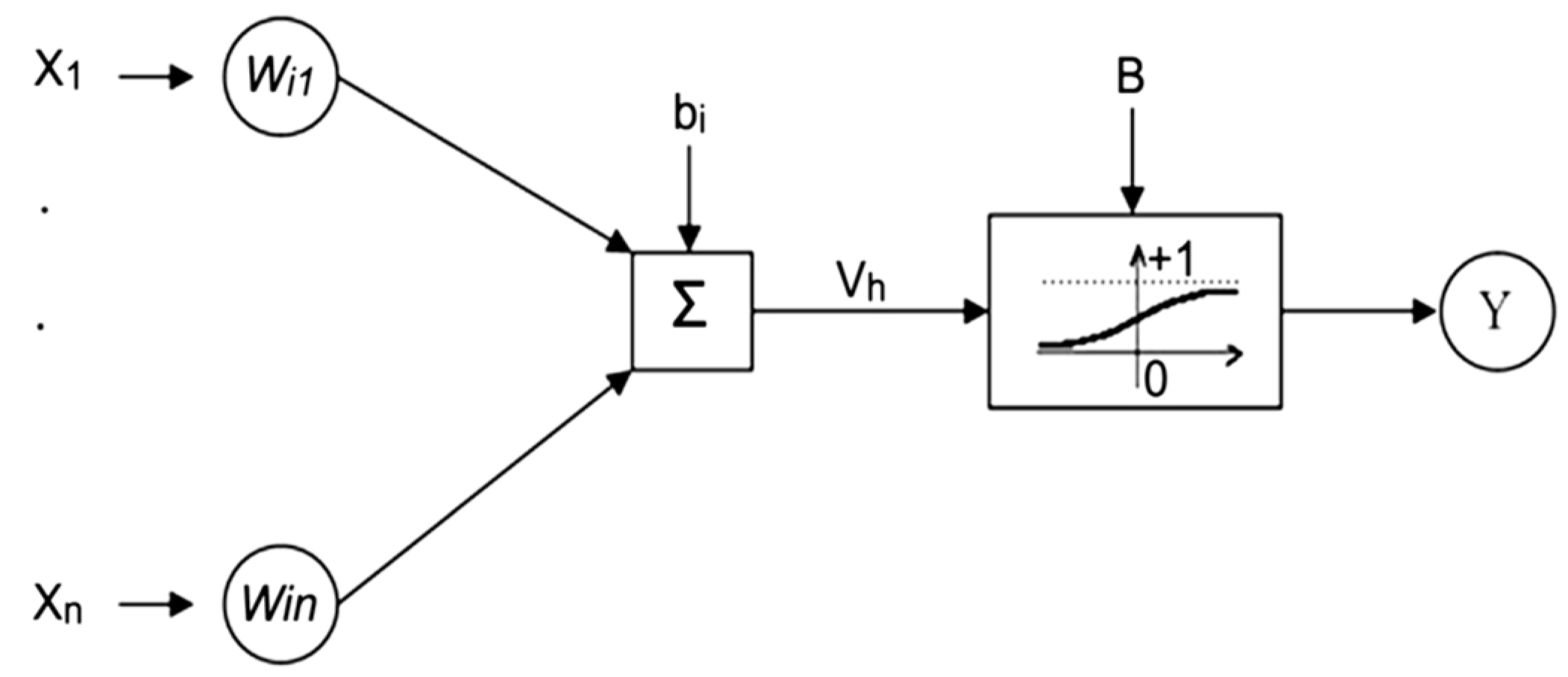
The MLP network consists of an input and output layer and at least one hidden layer. Each of these layers has several neurons and contains the processing unit (s), and each unit is fully connected to the next layer units by a weighted connection (W_ij) [23]. The Y output is obtained by transferring the sum of the previous outputs and mapping by an activation function. Figure 3 basically illustrates the multilayer perceptron neural network. In this figure, X_i represents the inputs, and b/B represents the bias between the different layers. For complex and nonlinear problems, the hyperbolic tangent function or the sigmoid (or log-sigmoid) function can be used.

A neural network is trained by a set of data called training data. During the training process, the weights of the network are optimized to reach the stopping criteria. The training process has two basic steps, whereby the first step is to give the initial values to the system (initialization), and the second step is optimization. In the initialization step, the initial values of weights and bias are allocated to neuron networks. Initial values of weights and bias can be obtained randomly or by using a global optimization method such as simulated annealing.

3.4. Support Vector Machine

The support vector machine, which was originally introduced by Boser et al. in 1992 [24], is inspired by the concept of statistical learning theory. To model the hydrodynamic behavior of the breakwater that is studied, the back-vector machine will be employed as a regression method by introducing an ε-insensitive loss of function. The following is a brief description of the use of a support vector machine in regression problems. For more information, refer to [25,26]. Consider a set of data for model training; {(x₁,y₁),…(x_n,y_n), x ϵ Rn, y ϵ r, where x is input, y is output, R_n is the n-dimensional vector space, and r is the one-dimensional vector space. The ε-insensitive loss of function can be expressed as follows:

$${\mathrm{L}}_{\mathsf{\epsilon }}\left(\mathrm{y}\right)=0 \mathrm{For} \left|\mathrm{f}\left(\mathrm{x}\right)-\mathrm{y}\right|{< \mathsf{\epsilon } \mathrm{or} \mathrm{L}}_{\mathsf{\epsilon }}\left(\mathrm{y}\right)=\left|\mathrm{f}\left(\mathrm{x}\right)-\mathrm{y}\right|-\mathsf{\epsilon }$$

(5)

This expression defines a ε-domain such that if the predicted value is in the domain, the loss is zero, while if the predicted value is outside the domain, the loss will be equal to the absolute value of standard deviation subtract ε. The primary purpose of a vector machine is to find a function f (x) that gives the deviation of ε from the actual output value and is uniform.

The final Equation in the support vector machine can be written as follows [25]:

$$\mathrm{f}\left(\mathrm{x}\right)={{\displaystyle \sum }}_{\mathrm{i}=1}^{\mathrm{nsv}}\left({\mathsf{\alpha }}_{\mathrm{i}}-{\mathsf{\alpha }}_{\mathrm{i}}^{*}\right)\mathrm{K}\left({\mathrm{x}}_{\mathrm{i}}{,\mathrm{x}}_{\mathrm{j}}\right)+\mathrm{b}.$$

(6)

In the above relationship, αi and αi * are Lagrangian coefficients, nsv is the number of supporting vectors, and K(x_i,x_j) is a kernel function. Some common kernels such as homogeneous and non-homogeneous polynomials, radial basis function, and Gaussian function. In the present study, Gaussian, linear, quadratic, and cubic kernel functions are used to investigate the model.

3.5. Gaussian Process Regression

Gaussian process regression (GPR) models are probabilistic models based on non-parametric kernels. Consider the training dataset {(x_i, y_i); i = 1, 2, …, n} such that x_i ∈ ℝ^d and y_i ∈ ℝ are derived from an unknown distribution. A GPR model with respect to the new input vector x_new and the training data supports the prediction of the variable response value of y_new. A linear regression model is as follows:

y = x^Tβ + ε

(7)

where $\mathrm{\epsilon }~\mathrm{N}\left(0,{\mathrm{\sigma }}^2\right)$. The error variance σ² and the coefficient β are calculated from the data. A GPR model describes the response by introducing latent variables from a Gaussian process, f(x_i), i = 1,2, …, n, and the explicit basic functions h. The covariance function of the hidden variables introduces smoothness of the response, and the base functions transfer the inputs of X to a p-dimensional feature space. A Gaussian process is a set of random variables such that any finite number of them, have a Gaussian distribution. If {f(x),x∈ℝd} is a Gaussian process and n has observations x₁, x₂, …, x_n, the distribution of random variables f (x₁), f (x₂), …, f (x_n) is also Gaussian. A Gaussian process is defined by the mean function m(x) and the covariance function k (x, x′). That is, if {f(x),x∈ℝd} is a Gaussian process, then E(f(x)) = m(x) and Cov[f(x),f(x′)] = E[{f(x)−m(x)}{f(x′)−m(x′)}] = k(x,x′). Now consider the following model:

h(x)^Tβ + F(x)

Therefore, f(x)~ Gaussian process (0, k(x,x′)), which means that f (x) is obtained from a Gaussian process with a mean of zero and the covariance function of c(x, x′). h (x) is a set of basic functions that transfers the original feature vector x from Rd to the new feature vector h (x) in Rd. β is a p-by-1 vector of the coefficients of the base functions. This model represents a GPR model. An example of a response y can be modeled as follows:

$$\mathrm{P}\left({\mathrm{y}}_{\mathrm{i}}{\left|\mathrm{f}\right(\mathrm{x}}_{\mathrm{i}}{),\mathrm{x}}_{\mathrm{i}}\right)~\mathrm{N}({\mathrm{y}}_{\mathrm{i}}{\left|\mathrm{h}\right(\mathrm{x}}_{\mathrm{i}}{)}^{\mathrm{T}}\mathsf{\beta }+\mathrm{f}\left({\mathrm{x}}_{\mathrm{i}}\right){,\mathsf{\sigma }}^2)$$

Hence, a GPR model is a probabilistic model. The hidden variable f (x_i) is introduced for each xi observation, which makes the GPR model non-parametric [27].

3.6. Genetic Programming

GP was originally inspired by the evolution process [27] An individual program refers to a parse tree that consists of functions (nodes) and terminals (leaves). A function set may include mathematical functions (such as sin, cos, sqrt, exp), mathematical operators (+, $-$, ÷, ×), Boolean operators, conditional functions, iterative functions, and any user-defined functions. Also, a terminal set, contains independent variables, dependent variables, random coefficients, and constant values.

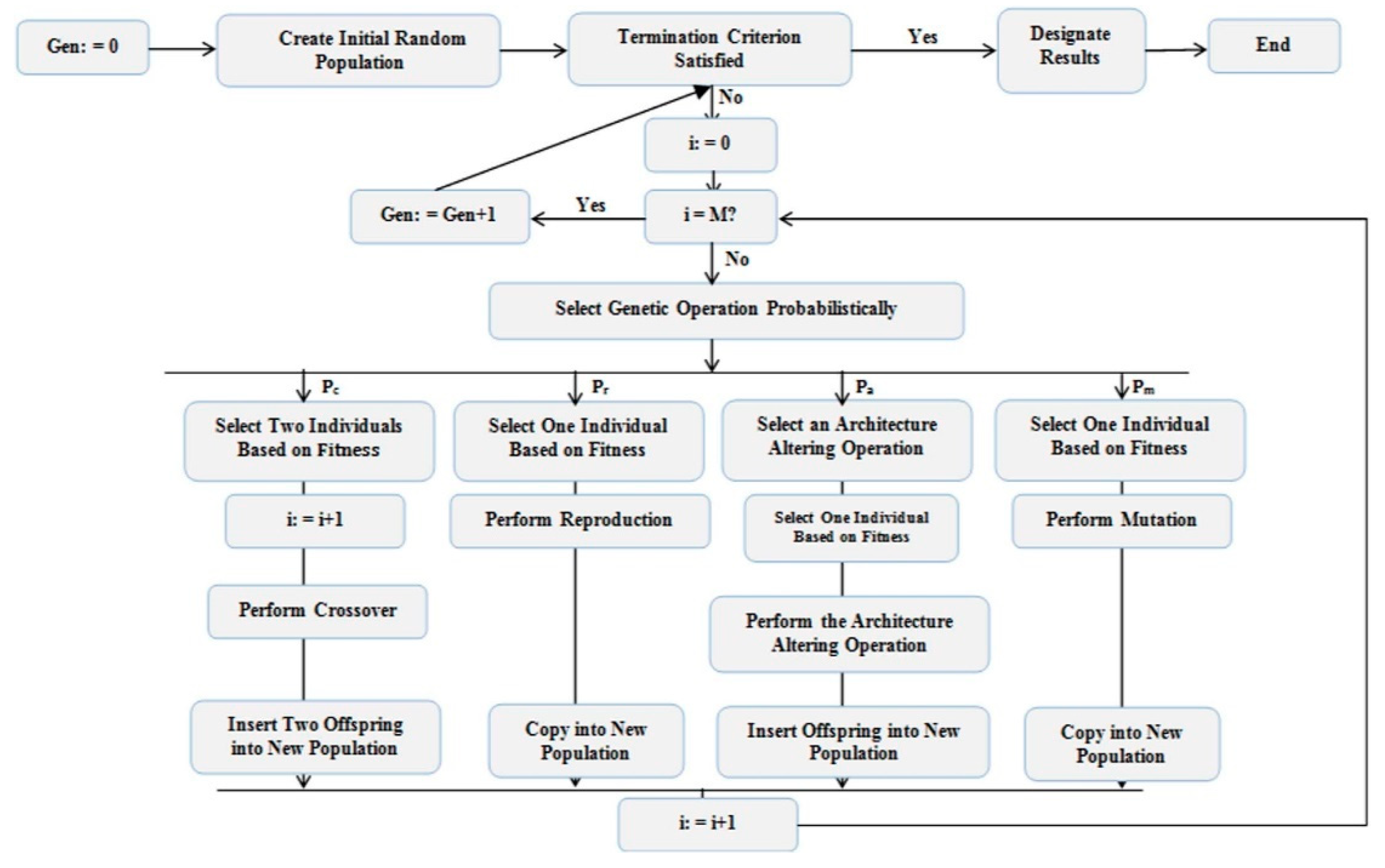
Producing the final result, called solution in GP, was achieved by performing the following step-by-step procedure. As indicated in Figure 4, initial models (populations) are randomly created from the terminal set and function set. Each model (individual) is evaluated based on defined statistical criteria such as RMSE to select next-generation parents. Then, GP uses selection methodologies, such as ranking, to randomly pick up a certain number of the fittest models at several times to select the next-generation parents. Next-generation offspring are produced using GA operators such as reproduction, crossover, and mutation. This will continue until the termination condition means the number of generations or the desired accuracy.

According to the above mentioned, the following steps should be taken to create a model in GP [28]: (1) Specify the terminal set. (2) Choose the appropriate functional set. This step can be challenging and misleading as choosing the wrong functions can lead to models that are not physically sound. In this paper, the functional set is selected based on trial and error. (3) Determine a fitness criterion to evaluate the accuracy of models. This criterion determines which models survive to produce the next generation. In this study, root mean square error (RMSE) was used as a fitness criterion. (4) Specify the model controlling parameters. This parameter includes gene linking function, GP operators, and chromosomes. These parameters are capable of controlling the size and accuracy of models and, if not considered, can produce nested models that are hard to interpret and computationally expensive. (5) Criterion for termination conditions: This criterion is specified in either the number of generations or the specific accuracy achieved.

4. Modeling of Reflection and Transmission Coefficients

According to the above, reflection and transmission coefficients play a key role in determining the behavior of permeable-type breakwaters. Reflection and transmission coefficients have been expressed in many studies as a function of wave variables such as wavenumber and wave steepness and main breakwater characteristics such as chamber width and wall permeability. It is also shown in these studies that some parameters like panel thickness, the shape of vertical panel piles, and their roughness have a secondary influence or no specific influence on the hydrodynamic behavior of permeable-type breakwaters [2,29,30].

In this study, due to the use of rockfill materials in the absorber chamber, the height of rockfill materials has been considered as a parameter for the first time. The other most important parameters affecting the behavior of reflection and transmission coefficients are selected by reviewing the technical literature related to the permeable breakwater. As a result, the relationship between the reflection and transmission coefficients can be expressed as follows:

$${\mathrm{C}}_{\mathrm{t}}{, \mathrm{C}}_{\mathrm{r}}=\mathrm{f}(\frac{\mathrm{B}}{\mathrm{h}},\frac{\mathrm{d}}{\mathrm{h}},\frac{\mathrm{B}}{{\mathrm{L}}_{\mathrm{p}}},\frac{{\mathrm{H}}_{\mathrm{s}}}{{\mathrm{L}}_{\mathrm{p}}}, \mathrm{Kh},\frac{{\mathrm{H}}_{\mathrm{s}}}{\mathrm{d}},\mathrm{p})$$

(8)

where C_t and C_r, respectively, are transmission and reflection coefficients, B is the width of breakwater chamber (distance between front and back panel), h is the depth of water, d is the height of rockfill materials, L_p is wavelength associated with peak period (T_p) wave spectrum, H_s significant wave height of wave spectrum, K is wave number or angular frequency (is equal to $\frac{2\mathsf{\pi }}{{\mathrm{L}}_{\mathrm{p}}}$), and p is the permeability of the back wall, defined as the ratio of permeable wall openings to the entire vertical surface of the wall from the water surface to the bed of the flume. Previous studies on Jarlan’s multi-layer breakwaters without the use of rockfill materials have suggested that the presence of a back wall with less porosity compared to the front wall will improve the performance of the breakwater [31,32]. In some other studies on multi-layer permeable breakwater, it has been shown that if the back wall has more than 40% porosity, it is ineffective. Given the fact that the introduced breakwater behaves differently from the previous breakwaters due to the presence of rockfill material in its core, this study seeks to investigate the effect of back wall porosity on suggested breakwater [33,34].

The water depth is assumed to be constant and 40 cm in all tests. Table 1 gives definitions and ranges of input parameters that are summarized for the main model used in experiments.

4.1. Data and Preprocessing

The experimental data were used to develop the model. The database covers a wide range of parameters influencing the reflection and transmission coefficients. The database consisting of 360 records and predictors in this study are relative chamber width (B/h), relative rockfill height (d/h), relative chamber width in terms of wavelength (B/L_p), wave steepness (H_s/L_p), wave number multiplied by water depth (kh), and relative wave height in terms of rockfill height (H_s/d). The primary purpose of using dimensionless parameters is to apply the results of a smaller-scale physical model to real work. Selected parameters have been considered and applied previously in several studies related to permeable breakwater [3,4,9] and have specific concepts in coastal engineering. For example, investigating the effect of H_s/L_p and kh on C_t and C_r is essential to understand the hydrodynamic characteristics of the present breakwater for coastal and deepwater regions. Also, investigating the effect of B/L_p, $\mathrm{d}/\mathrm{h}, \mathrm{B}/\mathrm{Lp}$, H_s/d, and P on C_t and C_r is required to select the appropriate and optimized structure configuration.

The porosity of the rockfill material was initially considered as the parameter candidate. However, in later studies, it was found that there are two limitations to the nominal size of the rocks. First, the size of the rocks must be large enough to prevent them from coming out of the front and back walls. Second, the limitations related to the implementation and supply of material issues, which limits the size of the rocks. With these two limitations, the range of porosity of the rocks is practically low and, therefore, it is not considered as a parameter. The effect of the shape and porosity of the materials may be studied by using concrete block armor with different shapes and porosities and can be the subject of future studies.

Table 2. Definitions and ranges of scaled model parameters.

Parameter	Definition	Range	Average	Standard Deviation
P	Back wall porosity (%)	30–50	40	10
B/h	Relative chamber width	0.4–2	1.2	0.57
d/h	Relative rockfill height	0.75–1.4	1.09	0.24
B/Lp	Relative chamber width in terms of wavelength	0.03–0.86	0.19	0.15
Hs/d	Relative wave height in terms of rockfill height	0.05–0.45	0.18	0.09
Kh	The wavenumber multiplies the water depth	0.49–2.96	1.01	0.57
Hs/Lp	Wave steepness	0.01–0.06	0.03	0.01
Cr	Reflection coefficient	0.16–0.54	0.37	0.09
Ct	Transmission coefficient	0.11–0.77	0.44	0.1

summarizes the definitions and ranges of input parameters of the original model used in the experiments and shows the domain of model parameters and the standard deviation.

A cross-validation statistical method was used to evaluate the performance of machine learning models. This method is commonly used in machine learning approaches to compare and select a model in a predictive modeling problem, due to its ease in understanding, implementation, and in estimating modeling skills. In general, this method is considered to be less biased over other methods. This approach involves randomly dividing the dataset into K_c groups or folds of approximately equal size. The first fold is treated as a validation set (testing), the modeling is fitted to the remaining (K_c – 1) folds, and this partition is applied until each fold is tested one time and will continue (K_c − 1) times to fit the model [35].

Poor selection of K_c may lead to a false idea of the model skill level, such as having a high variance score (which may vary greatly based on the data used to fit the model) or high bias (which may be due to overestimating the model’s skills). K_c is usually 5 or 10, but there is no formal rule. As K_c increases, the difference between training datasets and subsequent iterations subsets becomes smaller. As the difference decreases, the bias becomes smaller. In this study, considering the number of data, k is equal to 8 (28). As a result, from a total of 360 sets of lab results, 315 datasets in 7-fold were used for the training process, and 45 were used in each step for model testing.

In the case of multilayer perceptron neural network, due to its nature instead of using the cross-validation method, the data are divided into three sections: training, validation, and testing with ratios of 70%, 15%, and 15%, respectively, and after constructing the model, its features are obtained. The number of datasets for training, validation, and testing data are 252, 54, and 54, respectively.

Frank and Todeschini (1994) proposed a minimum ratio of data number to the number of input variables to accept the model, which is 3, and also recommended that this ratio be greater than 3 [36]. In the present study, this ratio for the training and test datasets is 315/3 = 105 and 45/3 = 15, respectively, both of which are much higher than the proposed ratio.

For the neural network model, this ratio for training, validation, and test data are 252/3 = 83, 54/3 = 18, and 54/3 = 18, all of which are much higher than the proposed ratio.

4.2. Performance Measurement

Correlation between model outputs and measured values that are expressed by the correlation coefficient is one of the important tools in evaluating the predictive performance of a machine learning model.

Whenever the correlation coefficient is closer to one, the model is more correlated to the actual results. According to a rational principle, Smith stated that, if a model had a correlation coefficient of more than 0.8 (R > 0.8), there was a strong correlation between the model output and the actual results [37].

Another indicator of model performance is the prediction error rate of the models, which are mean absolute error (MAE) and root mean square error. Finally, the optimal model is selected based on two objectives:

(1)

Provide the best correlation expressed by the correlation coefficient

(2)

Provide the least error represented by the RMSE index

For this purpose, the following objective function is used to satisfy both goals simultaneously. Then, choosing the optimal model is achieved by minimizing the following objective function.

$$\mathsf{\rho }=\frac{\mathrm{RMSE}}{{\overline{\mathrm{h}}}_{\mathrm{i}}}\frac{1}{\mathrm{R}+1}$$

(9)

where ${\overline{\mathrm{h}}}_{\mathrm{i}}$ is the mean of the predicted values for the reflection and transmission coefficients. Due to the lack of a definitive evaluation criterion [38], in addition to the correlation coefficient, RMSE, and objective function, several statistical indicators, including the relative error (RE) or index of agreement, the scatter index (SI), and the Nash–Sutcliffe efficiency coefficient (E). have been used to evaluate the performance of the models. In general, when the values of RE and E are close to 1, the model has a better predictive performance. Conversely, the lower the value of SI, the better agreement between predicted and measured values [39,40].

The R, RMSE, MAE, RE, SI, and E functions can be found in the Appendix A.

5. Results and Comparison

5.1. Comparison of Models and Model Selection

In this study, 20 linear and nonlinear regression models for modeling hydrodynamic behavior of breakwater using the parameters listed in Table 2. The results for the RMSE, R, and ρ models are presented in

Table 3. Proposed ML regressors and their result for the reflection coefficient.

ML Regressor		Reflection Coefficient
	E	Relative Error (RE)	Scatter Index (SI (%))	RMSE	R Squared	OBJ Function (ρ)
Linear Regression	0.8363	0.9536	9.7	0.036794	0.83	0.0520
Interactions Linear	0.9348	0.9970	6.1	0.025197	0.92	0.0348
Robust Linear	0.8360	0.9821	9.7	0.036859	0.83	0.0521
Stepwise Linear	0.9259	0.9957	6.5	0.025446	0.92	0.0351
Fine Tree	0.9751	0.9979	3.8	0.025985	0.92	0.0358
Medium Tree	0.9494	0.9967	5.4	0.029467	0.89	0.0410
Coarse Tree	0.8825	0.9909	8.2	0.035110	0.85	0.0494
Linear SVM	0.8355	0.9886	9.7	0.036758	0.83	0.0520
Quadratic SVM	0.9476	0.9960	5.5	0.023015	0.93	0.0317
Cubic SVM	0.9679	0.9977	4.3	0.022148	0.94	0.0304
Medium Gaussian SVM	0.9712	0.9979	4.1	0.021394	0.94	0.0294
Coarse Gaussian SVM	0.8647	0.9899	8.8	0.033973	0.86	0.0476
Boosted Trees	0.9358	0.9954	6.1	0.026707	0.91	0.0369
Bagged Trees	0.9582	0.9969	4.9	0.024971	0.92	0.0344
Squared exponential GPR	0.9730	0.9981	3.9	0.020357	0.95	0.0279
Matern 5/2 GPR	0.9797	0.9985	3.4	0.020222	0.95	0.0277
Exponential GPR	0.9999	0.9999	0.014	0.019949	0.95	0.0273
Rational Quadratic GPR	0.9753	0.9982	3.8	0.020366	0.95	0.0279
GP	0.9207	0.9940	6.7	0.025117	0.92	0.0346
ANN	0.9100	0.9935	7.2	0.026791	0.91	0.0370

and

Table 4. Proposed ML regressors and their result for the transmission Coefficient.

ML Regressor	Transmission Coefficient
	E	Relative Error (RE)	Scatter Index (SI (%))	RMSE	R Squared	OBJ Function (ρ)
Linear Regression	0.7960	0.9404	15.10	0.069152	0.78	0.0835
Interactions Linear	0.9448	0.9856	7.85	0.039621	0.93	0.0458
Robust Linear	0.7826	0.9356	15.58	0.071068	0.77	0.0860
Stepwise Linear	0.9423	0.9849	8.02	0.038990	0.93	0.0451
Fine Tree	0.9810	0.9951	4.60	0.038005	0.93	0.0440
Medium Tree	0.9489	0.9867	7.55	0.043723	0.91	0.0509
Coarse Tree	0.8740	0.9654	11.86	0.065657	0.81	0.0785
Linear SVM	0.7866	0.9357	15.44	0.070599	0.78	0.0852
Quadratic SVM	0.9584	0.9893	6.82	0.034423	0.95	0.0396
Cubic SVM	0.9806	0.9950	4.65	0.027994	0.96	0.0321
Medium Gaussian SVM	0.9804	0.9948	4.67	0.033301	0.95	0.0383
Coarse Gaussian SVM	0.8351	0.9487	13.57	0.064471	0.81	0.0771
Boosted Trees	0.9608	0.9894	6.61	0.034954	0.95	0.0402
Bagged Trees	0.9705	0.9919	5.74	0.037562	0.94	0.0433
Squared exponential GPR	0.9897	0.9974	3.38	0.024612	0.97	0.0282
Matern 5/2 GPR	0.9945	0.9986	2.47	0.024526	0.97	0.0281
Exponential GPR	0.9999	0.9999	0.02	0.023402	0.98	0.0267
Rational Quadratic GPR	0.9931	0.9982	2.76	0.024767	0.97	0.0284
GP	0.9195	0.9784	9.48	0.042169	0.94	0.0487
ANN	0.9383	0.9838	8.3	0.036900	0.94	0.0426

. The results show that, for the Cr output for the whole exponential Gaussian process model dataset, the least error and highest correlation are obtained simultaneously, and the objective function value has the lowest value, 0.0273. It is also evident that linear, linear SVM, and robust linear models are less capable of predicting the pass-through coefficient, although other GPR models perform well near the exponential Gaussian process model.

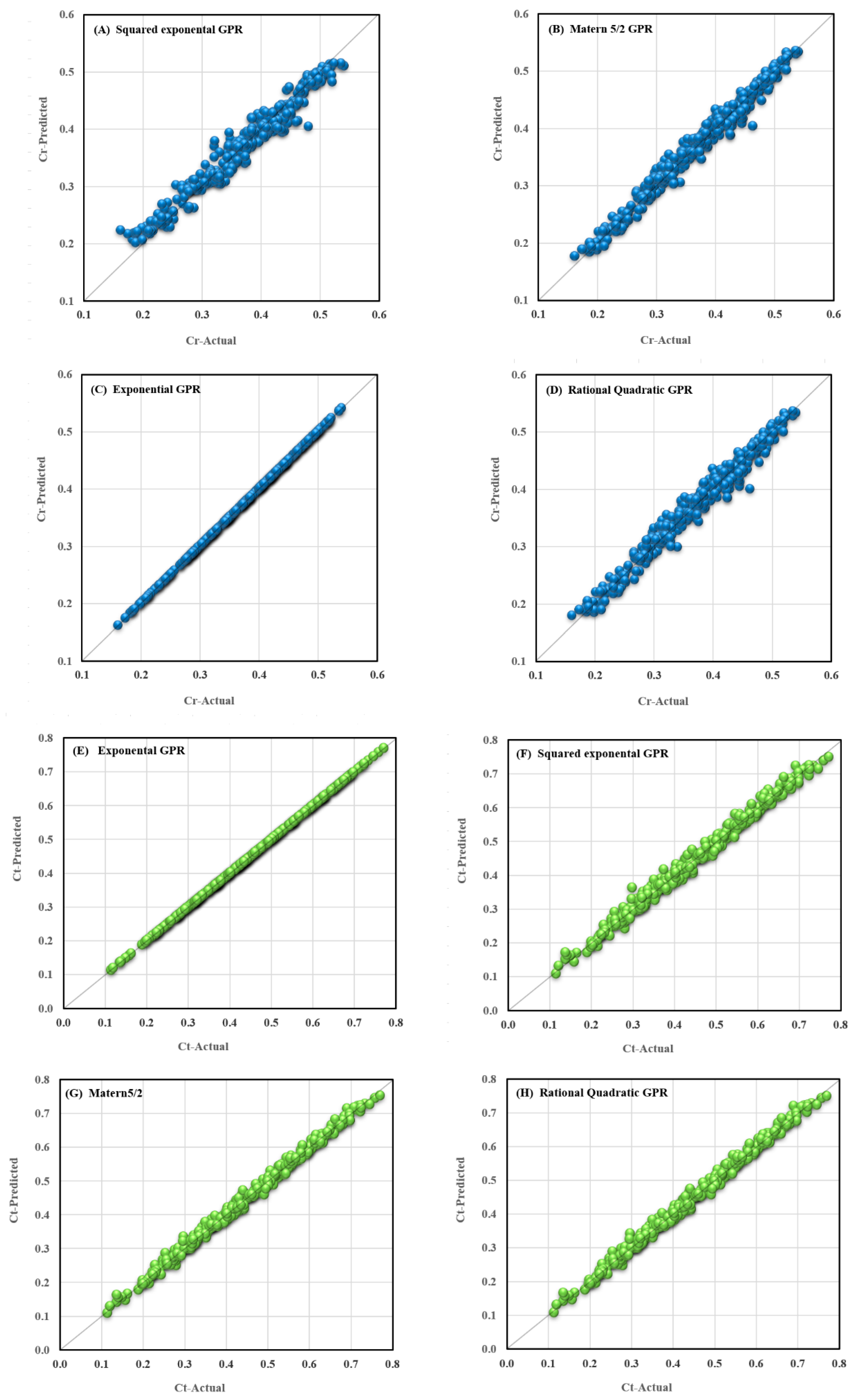
In the case of the Ct output, similarly, the exponential Gaussian process model has the least error and the highest correlation, and its objective function value is 0.0267, which is the least value. Concerning the target parameter, Ct, linear, linear SVM, and robust linear models are also weaker than other models, and other GPR models include squared exponential, matern5/2, and rational Quadratic models demonstrate the best performance after the exponential GPR model.

Therefore, according to the introduced objective function and the numbers obtained in Table 3 and Table 4, the exponential Gaussian process model is generally the best model to predict the reflection and transmission coefficients. The prediction results of the top four models of each output are also visualized in Figure 5.

The introduced innovative breakwater has not been studied before, and therefore there are no empirical equations in predicting reflection and transmission coefficients as a reference for engineers in practical work. As indicated in Section 3, in contrary to most machine learning approaches, genetic programming represents an explicit functional relationship between input and output variables. Using this capability, the following formula has been developed respectively for reflection and transmission coefficients:

$$\begin{array}{cc}\hfill \mathrm{Cr}& =\frac{\mathrm{d}}{4\mathrm{h}}+{\left(\frac{\mathrm{d}}{\mathrm{h}}\right)}^{0.2}+\frac{\left(\frac{{\mathrm{H}}_{\mathrm{s}}}{{\mathrm{L}}_{\mathrm{p}}}\right)}{2\times \left(\mathrm{Kd}\right)}+\frac{(\mathrm{Tan}\mathrm{h}\left(\frac{\mathrm{B}}{\mathrm{h}}\right)-\left(\frac{\mathrm{B}}{{\mathrm{L}}_{\mathrm{p}}}\right)+1)}{16.85 \times \mathrm{Kd}}\hfill \\ & -1.3 \times {\left[{\left(\frac{\mathrm{d}}{\mathrm{h}}\right)}^2 \times \mathrm{kd} \times \left(\mathrm{Arctg}\left(\frac{\mathrm{d}}{\mathrm{h}}\right)-1\right) \times \left(\frac{{\mathrm{H}}_{\mathrm{s}}}{\mathrm{d}}+\frac{{\mathrm{H}}_{\mathrm{s}}}{{\mathrm{L}}_{\mathrm{p}}}\right)\right]}^{\left(\frac{1}{15}\right)}-2.07\hfill \end{array}$$

(10)

$$\begin{array}{cc}\hfill \mathrm{Ct}& =\mathrm{Arctg}{\left[{\left(\frac{\mathrm{d}}{\mathrm{h}}\right)}^3-{(2.07 \times \mathrm{kd} \times \mathrm{Ln}\left(\frac{\mathrm{d}}{\mathrm{h}}\right))}^{\left(\frac{1}{3}\right)})\right]}^{0.2}+{\left[(0.31 \times \frac{\mathrm{B}}{{\mathrm{L}}_{\mathrm{p}}}\right)-\left(3.06 \times \frac{{\mathrm{H}}_{\mathrm{s}}}{{\mathrm{L}}_{\mathrm{p}}}\right)+\frac{{\left(\frac{\mathrm{B}}{\mathrm{h}}\right)}^{0.2}}{(2\times \frac{\mathrm{d}}{\mathrm{h}})}]}^9\hfill \\ & -{(\frac{\mathrm{B}}{\mathrm{h}})}^{0.25} \times (\frac{{\mathrm{H}}_{\mathrm{s}}}{{\mathrm{L}}_{\mathrm{p}}}{)}^{0.2} \times (\frac{\mathrm{d}}{\mathrm{h}}) \times \mathrm{Tanh}(\frac{{\mathrm{L}}_{\mathrm{p}}}{11.41 \times {\mathrm{H}}_{\mathrm{s}}})\hfill \end{array}$$

(11)

Although GP models are not among the best-performing models, they still demonstrate a robust performance, according to Smith [38] (see Table 3 and Table 4), and can be a guide for engineering purposes for both targets. By looking at Equations (10) and (11), it could be found that the parameter P is not present in the Equations, and it probably implies that the reflection and transmission coefficients are not sensitive to this parameter. In the sensitivity analysis section, the relationship between model parameters and outputs is examined in detail.

5.2. Parameter Settings of Selected Models

To obtain effective parameter settings, several performances with different parameters have been performed, and the best parameters have been selected based on the trial and error approach and the values recommended in previous studies. The parameters of the exponential Gaussian process for the modeling of both targets are shown in

Table 5. Parameters setting of the exponential GPR in the modeling of reflection and transmission coefficients.

Target	Parameter	Value
Reflection coefficient
	Kernel Function	Exponential
	Kernel Scale	1.664473
	Basic Function	Constant
	Signal Standard Deviation	0.063185
	sigma	0.063185
Transmission coefficient
	Kernel Function	Exponential
	Kernel Scale	1.664473
	Basic Function	Constant
	Signal Standard Deviation	0.105257
	sigma	0.105257

.

5.3. Selected Models

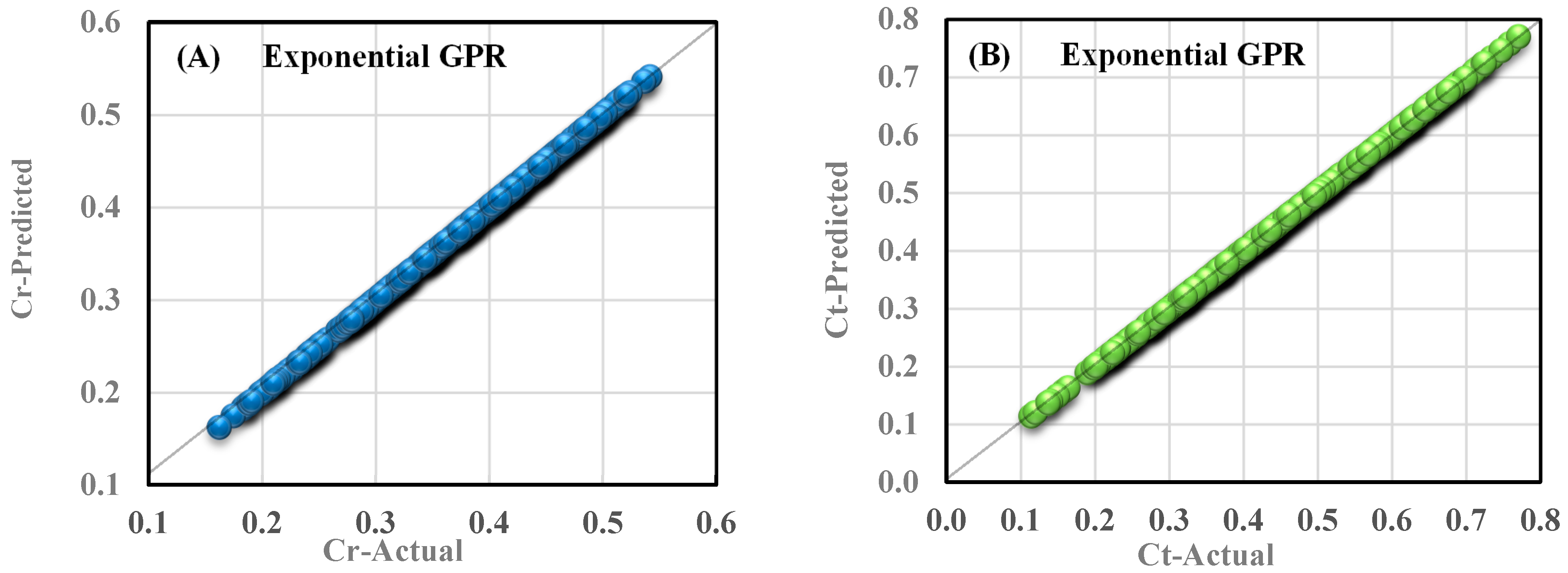
After evaluating the models through cross-validation, the exponential Gaussian process models are proposed to predict the behavior of reflection and transmission coefficients. A comparison of the predicted values of reflection and transmission coefficients with the experimental data for the preferred models is shown in Figure 6. It should be noted that the results shown in Figure 6 correspond to one of the models extracted from the cross-validation method.

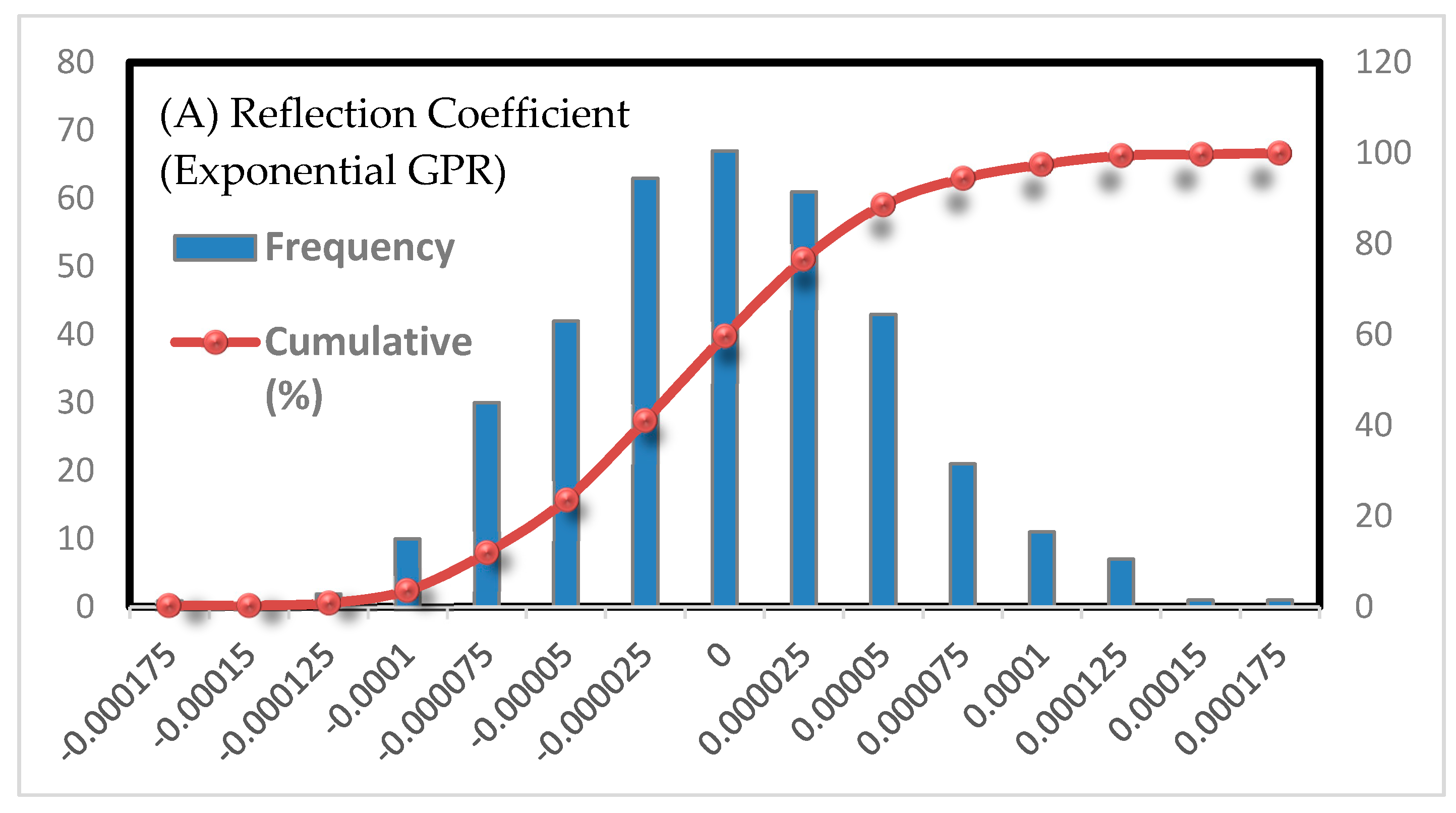
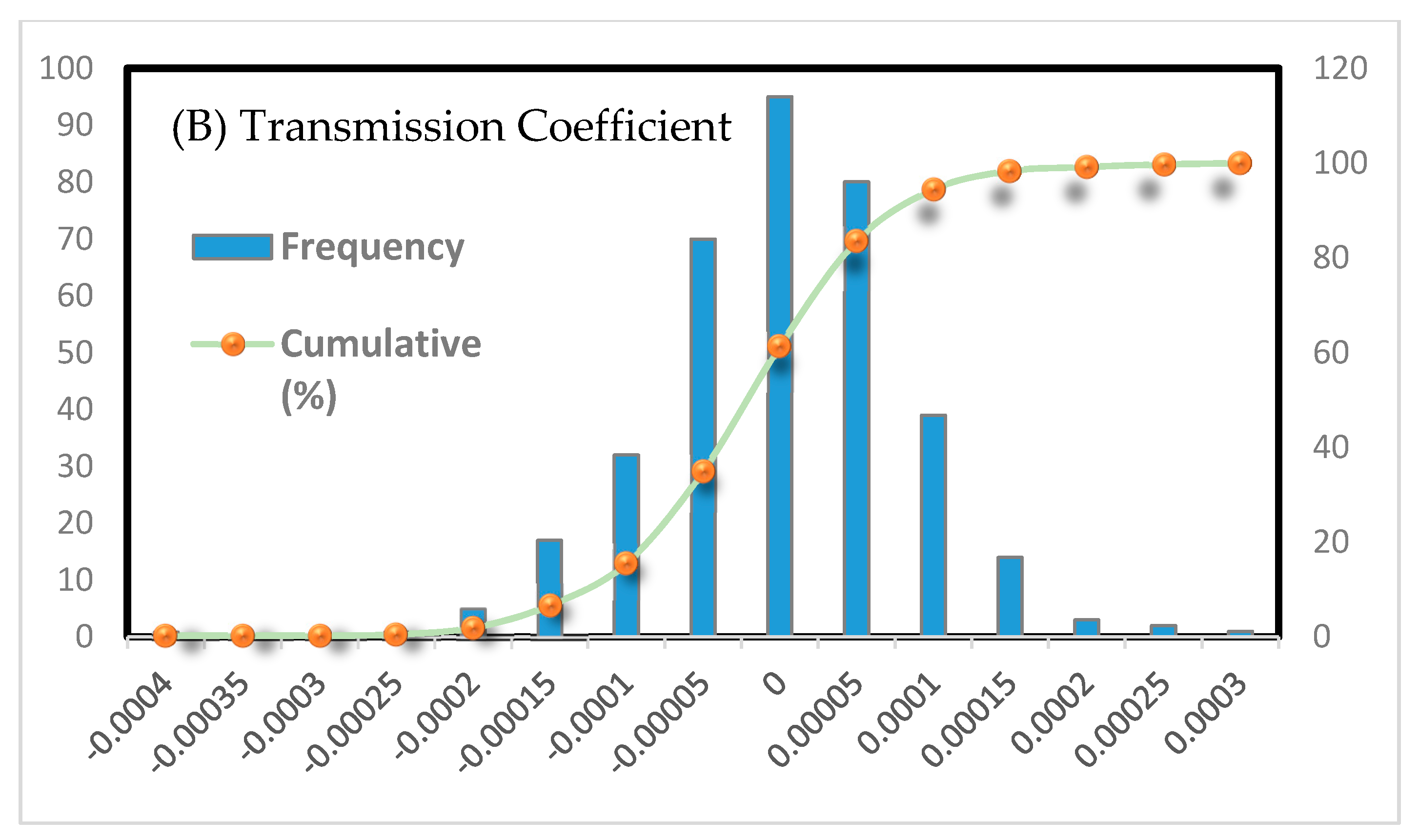
The error distribution of the predicted and actual values is shown in Figure 7. As can be seen, the noise is almost Gaussian (a normal distribution with mean zero), has a maximum of about zero, and has not deviated in any particular way. Also, the median (cumulative distribution of 0.5) is in the range of zero.

5.4. Sensitivity Study

Sensitivity analysis studies the contribution of input parameters in predicting outputs. A simple process was used to perform sensitivity analysis. The sensitivity percentage of output to each input parameter is obtained using the following Equations:

$${\mathrm{N}}_{\mathrm{i}}{=\mathrm{f}}_{\max }\left({\mathrm{x}}_{\mathrm{i}}\right)-{\mathrm{f}}_{\min }{(\mathrm{x}}_{\mathrm{i}})$$

(12)

$${\mathrm{S}}_{\mathrm{i}}=\frac{{\mathrm{N}}_{\mathrm{i}}}{{{\displaystyle \sum }}_{\mathrm{j}=1}^{\mathrm{i}}{\mathrm{N}}_{\mathrm{j}}} \times 100$$

(13)

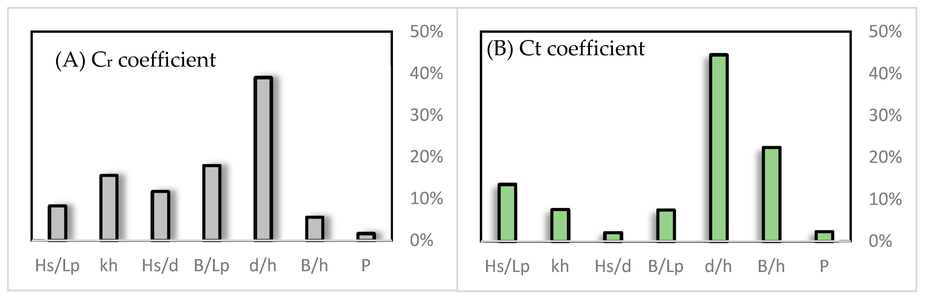
In the above Equations, ${\mathrm{f}}_{\max }\left({\mathrm{x}}_{\mathrm{i}}\right)$ and ${\mathrm{f}}_{\min }\left({\mathrm{x}}_{\mathrm{i}}\right)$ are the highest and the lowest predicted output values on the i-th input domain, respectively, so that the other parameters are equal to their mean values. The results of the sensitivity analysis of the model presented are shown in Figure 8.

For both reflection and transmission coefficients, the highest contribution is related to the d/h parameter, which is close to 40. From the outset, due to the importance of rockfill materials in eliminating wave energy and increasing wave resistance, this parameter was expected to have the greatest influence on the hydrodynamic behavior of the breakwater. Also according to previous studies, the probability of wave resonance at specified ratios (B/L_p = 0.5 + 0.5n) is another effective parameter in the reflection coefficient which is reflected in the B/L_p parameter.

However, the relative chamber width parameter (B/h) has little contribution to the reflection coefficient parameter, which means that the reflection coefficient is not sensitive to the breakwater width. Conversely, in the transmission coefficient case, the B/h parameter is the second most influential parameter. Changing the values of this parameter means increasing/decreasing the interaction of the incident wave with the rockfill materials in the absorber chamber that significantly leads to altering the wave energy, and consequently, the transmission coefficient. Another influential parameter is the wave steepness coefficient that is mentioned in previous studies. The least contributing parameter in both target coefficients is the permeability of the back wall, which may be related to slight variations in this parameter due to practical limitations (30%–50%).

6. Conclusions

In this study, 20 regression modeling methods, including linear and nonlinear models, have been used to model the hydraulic behavior of the innovative breakwater. The models presented are based on a database of 360 laboratory tests. The proposed models relate the reflection and transmission coefficients to seven dimensionless parameters ($\frac{\mathrm{B}}{\mathrm{h}}, \frac{\mathrm{d}}{\mathrm{h}}, \frac{\mathrm{B}}{{\mathrm{L}}_{\mathrm{p}}}, \frac{{\mathrm{H}}_{\mathrm{s}}}{{\mathrm{L}}_{\mathrm{p}}}, \mathrm{Kh}, \frac{{\mathrm{H}}_{\mathrm{s}}}{\mathrm{d}}, \mathrm{p}$). The results show that linear models are not capable of predicting reflection and transmission coefficients, but GPR models, especially exponential GPR, present highly correlated models. The values of the objective function for the coefficients of reflection and transmission are 0.0273 and 0.0267, respectively. Also, several statistical indices have been calculated for each model.

The error study also showed that the error distributions are approximately Gaussian, and the selected models are not biased. The sensitivity analysis of the models showed that the reflection coefficient model has the most sensitivity to the relative rockfill height (d/h) and the relative chamber width in terms of wavelength (B/L_p) parameters, and the back-wall porosity (P) parameter is the least important in this model. In the case of transmission coefficient modeling, the results show the sensitivity of the proposed model to the relative rockfill height (d/h) and the relative chamber width (B/h). Similarly, the model has the least sensitivity to the P parameter. Therefore, it has been concluded the wave hydrodynamic parameters (reflection and transmission coefficients) depend strongly on the relative rockfill height. In general, the reflection coefficient increases with the relative rockfill height (d/h), and conversely, the transmission coefficient decreases with an increasing relative rockfill height (d/h).

Providing the optimal model and examining the parameters influencing the model constitute an important tool for engineers in future studies. Furthermore, two explicit functional relationships are developed by utilizing the GP that can be used for practical purposes.