Topology Reconstruction of BIM Wall Objects from Point Cloud Data

Abstract

The processing of remote sensing measurements to Building Information Modeling (BIM) is a popular subject in current literature. An important step in the process is the enrichment of the geometry with the topology of the wall observations to create a logical model. However, this remains an unsolved task as methods struggle to deal with the noise, incompleteness and the complexity of point cloud data of building scenes. Current methods impose severe abstractions such as Manhattan-world assumptions and single-story procedures to overcome these obstacles, but as a result, a general data processing approach is still missing. In this paper, we propose a method that solves these shortcomings and creates a logical BIM model in an unsupervised manner. More specifically, we propose a connection evaluation framework that takes as input a set of preprocessed point clouds of a building’s wall observations and compute the best fit topology between them. We transcend the current state of the art by processing point clouds of both straight, curved and polyline-based walls. Also, we consider multiple connection types in a novel reasoning framework that decides which operations are best fit to reconstruct the topology of the walls. The geometry and topology produced by our method is directly usable by BIM processes as it is structured conform the IFC data structure. The experimental results conducted on the Stanford 2D-3D-Semantics dataset (2D-3D-S) show that the proposed method is a promising framework to reconstruct complex multi-story wall elements in an unsupervised manner.

1. Introduction

The production of as-built Building Information Modeling (BIM) databases from point cloud data is an important task in remote sensing. The target is to enrich the raw metric inputs with building component information which is crucial in navigation and scene interaction tasks [1,2]. The resulting data is also used by the Architectural, Engineering, Construction, Owner and Operator (AECOO) industry where it has proven to significantly facilitate refurbishment, facility management and project planning [3,4]. However, processing remote sensing data to BIM is a challenging task, especially without the use of prior knowledge about the environment. Various approaches are proposed to automate this procedure [5,6]. Typically, point cloud data is first produced of the scene by using static or dynamic data acquisition systems (Figure 1a). These raw inputs are processed by reasoning frameworks to segment basic primitives from the scene such as planes and cylinders and building component information is assigned to these primitives (Figure 1b). Next, the observed geometry is used to fill the voids in the point cloud by producing geometry in occluded areas i.e., connecting partially observed walls (Figure 1c). In a final step, the hierarchical relations and topology are defined between the building components, which in building environments is typically based on the Industry Foundation Classes (IFC) standard [7], which is the widely adopted implementation of BIM (Figure 1d). While the segmentation and subsequent classification are well researched topics, there is a lack of understanding of how to properly define topological relations between the observations and to fill the gaps in the point cloud with building information [8]. The aim of this research is to provide a more general and robust framework to reverse engineer these relations in building environments. More specifically, we target the reconstruction of the connections between observations of wall geometry that are highly occluded in the point cloud.

Current algorithms presented in the literature only partially solve the topology reconstruction. First of all, most approaches aim to retrieve geometric primitives instead of actual building component information such as defined by the IFC standard [9,10]. Consequently, these methods emphasize on processing the point clouds to static watertight models that only deal with superficial occlusions in the point cloud. The few methods that do reason about the structure of the building, i.e., how the observations relate to volumetric entities and their connections, are mostly limited by Manhattan-world scene assumptions which severely limit the method’s applicability. For instance, the methods of Becker et al. [11] and Tran et al. [12] only consider observations in orthogonal configurations. Another common abstraction is only considering the observed faces of straight walls. Even the promising methods of Ochmann et al. [13], Nikoohemat et al. [14] and the recent work of Tran et al. [15] are limited by these abstractions. To our knowledge, our approach is the only interpretation method that actively deals with more complex wall observations including those of curved and polyline-based walls, which are vital to a more complete processing of the point cloud.

Similarly, there is the limitation of the scope to a single building story, which ignores important multi-story remote sensing information. In previous work, we already proposed methods to perform the segmentation [16] and classification [17] on the entire dataset and we continue this approach for the topology reconstruction. Finally, there are few methods that consider the topology of the building components. Most methods are limited to a single connection type i.e., intersections between adjacent walls with exceptions such as Previtali et al. [18,19] and Jung et al. [20] who respectively also consider orthogonal and shortest Euclidean distance connections. In our work, we propose a framework that considers all three connection types and also blended connections for complex walls on multiple stories. To this end, we developed an unsupervised topology reconstruction method to process the point cloud to a more logical model with the proper semantics. In summary, our contributions are:

• The automated simultaneous processing of multi-story wall observations from point cloud data
• The development of a topology reconstruction framework that computes the best suited connection type in highly occluded areas
• The automated representation of complex building environments with straight, curved and polyline-based walls

The remainder of this work is structured as follows. In Section 2, the related work on BIM reconstruction is presented. Section 3 explains the methodology for the topology reconstruction of the partial wall geometry. The results of the investigation and the experiments are discussed in Section 4. The discussion is presented in Section 5. Finally, the conclusions and future work are presented in Section 6.

2. Background & Related Work

The reconstruction of the topology between wall observations is still a largely unexplored topic in the current literature as there are researchers that forego the topology reconstruction and leave this task up to the user [21]. We therefore expand our literature study to also include the topology reconstruction of rooms and other building components. There currently are three frequently used methods for topology reconstruction including cell decompositions, semantic nets with shape grammar and connection evaluations (Figure 2).

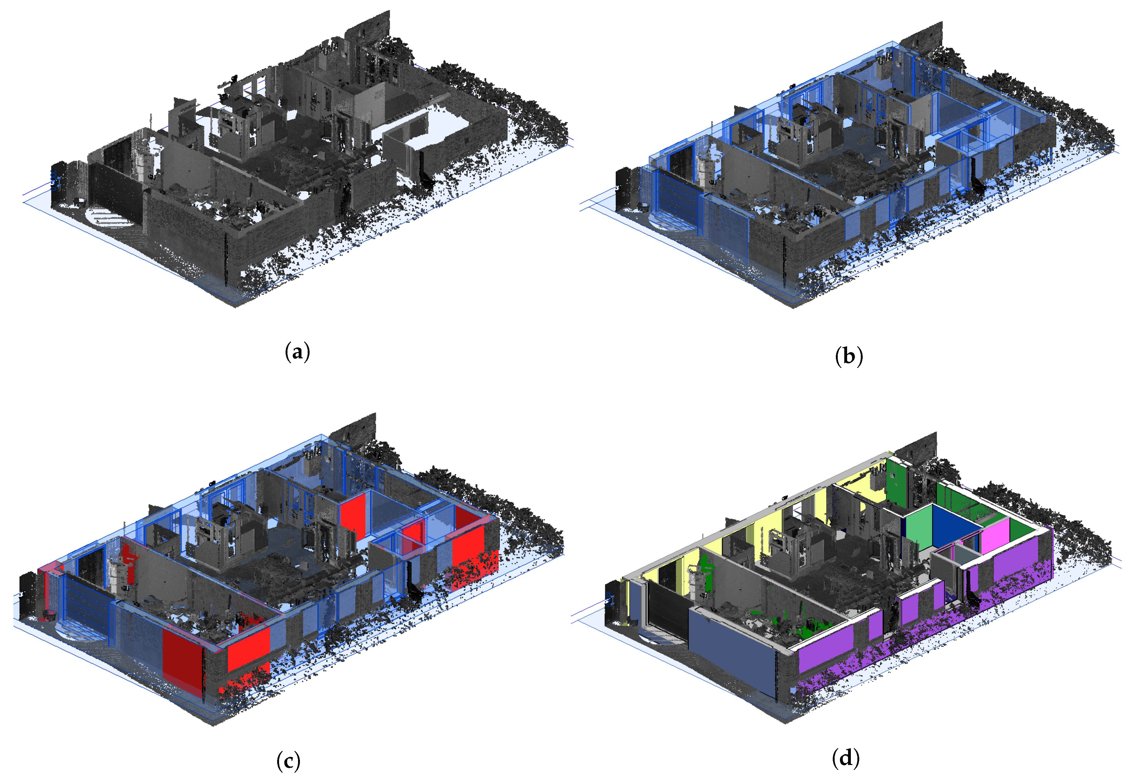
2.1. Cell Decomposition

Cell decompositions are the most commonly used method to create watertight room geometry and with it wall geometry. It extends the planar room boundaries to the edge of the bounding box of the building, thus creating a 2D or 3D cell grid of the structure. Following, the cells are merged together based on some seeding criteria such as the presence of floor or ceiling geometry. The naked edges of each cluster subsequently form the boundary of the room’s geometry. These boundaries can then be fused together and replaced with BIM wall objects. There are several researchers that show promising results with this technique for planar wall segments. Liu et al. [23], Turner et al. [24], Ambrus et al. [22], Budroni et al. [25] and Wang et al. [26] all use 2D or 2.5D cell decompositions for the production of accurate floor plans of a story. Mura et al. [10,27], Oesau et al. [9] and Xiao et al. [28] deploy 3D cell decompositions on an entire story and succeed in creating watertight BREP and CSG room volumes of the interior of a building. While their methods are designed to complete the topology of the boundaries of rooms, we believe it can be extended towards parametric wall reconstruction given a prior clustering of the wall segments and subsequently performing a cell decomposition on the candidate wall axes. Also, these methods show that topology reconstruction procedures significantly benefit from the incorporation of floor and ceiling information which we also use in our method.

While there are significant advantages to cell decompositions, there are several important limitations to consider. First, this method typically requires at least one observation from every wall in order to create proper cells. Also, appropriate seeding and the presence of ceiling or floor observations is required to properly detect the boundaries and the methods typically only operate on planar/linear segments. Typically, only intersecting connections are established in these methods that might fail to properly enclose the target space. Also, by considering every intersection between candidates, the combination complexity of $O\left(\right(n-1)!)$ quickly becomes overwhelming in larger datasets. Two very promising cell decompositions that overcome some of these obstacles are presented by Ochmann et al. [13] and Previtali et al. [19]. Both focus on optimizing the room layout but incorporate vital functionalities that we adopt for our wall topology reconstruction. Ochmann et al. pay close attention to the connections between neighboring rooms and deal with multi-wall intersections. Previtali et al., also consider orthogonal connections for the cell decomposition which increases the method’s robustness to occlusions. Overall, we adapt their functionalities but restrain from using cell decompositions because of the limited scalability due to the combination complexity. We opt for a more controlled influence zone of potential connections so we can consider more connection types.

2.2. Connection Evaluations

Connection evaluations are a more conventional approach to reconstruct the topology, but we believe, if implemented properly, it has very high potential. This framework, of which intersections are the most popular, evaluates potential connections between neighboring segments and connects them based on some evaluation criteria. For instance, Valero et al. [29] solve the intersections of pre-segmented wall lines to create an enclosed area. They retain the first intersection which scores well for single rooms with proper observations and so does Xiong et al. [30]. More recent implementations are presented by Nikoohemat et al. [14] and Murali et al. [31]. Nikoohemat merges parallel wallfaces into parametric volumes and intersects nearby volumes that lie within a certain Euclidean distance. Murali et al., extend their Manhattan-world planes and employ an adjacency graph based on the shortest Euclidean distance for the candidate selection. Neighboring walls that are near orthogonal are connected after which they complete the wall topology by testing the walls for Manhattan-world room layouts. An interesting method that could be considered as a connection evaluation is the skeleton line (wall axes) evaluation method of Jung et al. [20]. They iteratively connect adjacent wall axes by their shortest distance vector and condition these connections to not collide with floor or ceiling grid cells. In our work, we adapt the adjacency graph and the incorporation of ceiling and floor information but consider multiple connection types. This leads to a more informed decision framework on which connection is best suited between multiple wall axes lines and increases the applicability.

2.3. Shape Grammar

The use of shape grammar is becoming increasingly popular in reconstruction tasks. It is a top-down method that reconstructs elements conform a set of grammar rules. In the case of BIM, the IFC data structure along with common building logic is exploited to create instances of walls, rooms, doors and so on. For instance, Khoshelham et al. [32], Ikehata et al. [33], Becker et al. [11] and Tran et al. [34,35] all propose a grammar ontology for modeling indoor environments. Khoshelham et al., iteratively place, connect and merge navigable cuboid shapes, which is expanded by Tran et al., who propose additional rules for establishing adjacency, connectivity and containment relations between the reconstructed objects. A useful property of shape grammar is that the topology is used as prior information for the reconstruction and thus is inherently present in the model. Additionally, shape grammar can be used to predict the location of occluded rooms as shown in Tran et al. [34]. Given the proper structure grammar and operations, this technique has great potential for volumetric wall reconstruction. Especially the different types of connections are appealing to conduct a better informed reconstruction. Typically, these approaches are designed for room geometry and produce walls as a byproduct in the graph but this graph structure could potentially be reversed to process wall geometry. However, the current state of these methods are restricted to Manhattan-world scenes with orthogonal connections and straight walls. In this research, we propose a more general reconstruction but we do adapt the connectivity rules to decide which connection to chose to reconstruct the topology between multiple walls.

Surprisingly, multi-story reconstruction methods have only been proposed in the last several years such as in the method of Ochmann et al. [13]. 2D methods do not have a choice since they inherently make an abstraction of the dataset. However, 3D methods also generally pre-segment the point cloud into separate stories or rooms. In our 3D method, we specifically process multiple stories simultaneously since we strongly believe it contributes to the overall context and consistency of the model.

3. Topology Reconstruction

In this section, the BIM wall topology reconstruction pipeline is presented. The proposed approach focuses on the creation of a set of wall objects with the proper topological and hierarchical relations to complete the walls of the BIM model. Based on the literature, a connection evaluation methodology is proposed. This reduces the number of candidates compared to cell decompositions and offers a more flexible reconstruction framework compared to shape grammar which also allows us to test for multiple connection types. To the achievement of this goal, the following assumptions are made: (1) The point clouds are stored in a logical coordinate system, with the z-axis equal to the “up” direction, (2) the partial walls fit well to the IfcWallStandardCase definition and (3) the partial walls extracted in previous processes are correct.

The topology reconstruction consists of four steps (Figure 3). First, the neighboring wall axes to each wall end point are determined. Next, a set of potential connections is determined. In contrast to the literature, four potential connections are considered: intersecting connections, orthogonal connections, blended connections, which are a combination of the above, and direct connections, which are defined by the shortest Euclidean distance between the boundaries of the wall axes. Following, a unique set of connections is determined based on a cost function. In a final step, new IfcWallStandardCase objects are created and joined with the partial wall geometry to form a more logical BIM. Each step is discussed in detail below.

3.1. Preprocessing

The input of the pipeline is a set of partial LOD200 IfcWallStandardCase objects which represent the visible parts of the point clouds’ wall observations (Figure 1a). These walls are reconstructed from mesh geometry in previous research [36] and are vertical entities with a uniform wall thickness without openings, protrusions or niches. The wall axes of these objects can be both straight edges, curves or polylines. Additionally, we also use the mesh wall, ceiling and floor segments, which are obtained from previous segmentation and classification procedures [16,17], to support the topology reconstruction.

Prior to the topology reconstruction, a set of IfcBuildingStorey and IfcSpace objects are established to support the proposed procedure. The IfcBuildingStorey objects are automatically created from the clustered heights of the classified floor and roof segments of the mesh. The wall axes of the partial walls are bound to these IfcBuildingStorey objects by their base and top constraints and are used to retrieve neighboring wall axes. As such, the wall axes at different stories are processed in parallel, making the method highly performant. Additionally, a set of IfcSpace placeholders is computed for the room geometry. Each ceiling is paired with an underlying floor and their combined convex hull geometry serves as the BREP representation of the IfcSpace placeholders.

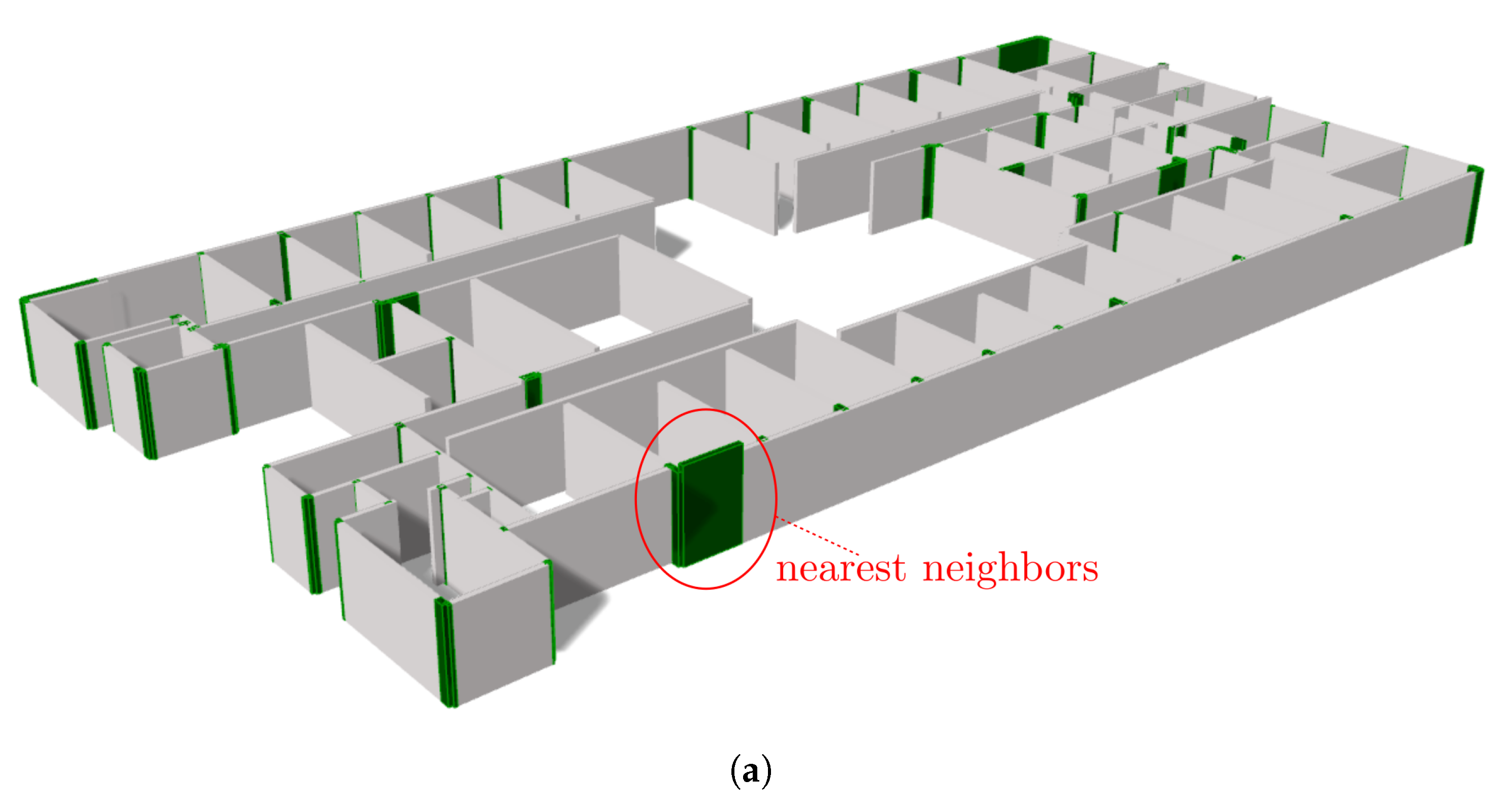
3.2. Neighbor Selection

The first step of the topology adjustment is creating an adjacency graph between neighboring partials wall axes based on the shortest Euclidean distance between the geometries. To determine which wall axes to connect, a set of seed points $\mathbf{P}$ are established (Figure 3a). Each endpoint of a wall axis $l_i\in L$ is considered a seed $p_i\in \mathbf{P}$ if it does not also belong to another wall axis. For a seed $p_i$ of a wall axis $l_i$, the wall axes $N_i$ are found so that each axes contains a point $q_j$ that lies within a user defined threshold distance $t_d$ of $p_i$ (Equation (1)). This Euclidean distance is set equal to the maximum gap a wall is allowed to span over to make a connection and is considered application dependent.

$$\begin{array}{cc}\hfill & \mathbf{P}=\left\{p_i\in l_i|l_i\in L,l_j\in L\backslash \left\{l_i\right\}:p_i\notin l_j\right\}\hfill \\ \hfill & N_i=\left\{l_j\in L\backslash \left\{l_i\right\}|\mathrm{d}(p_i,l_j)\le t_c\right\}\hfill \\ \hfill & Q_i=\left\{q_j\in l_j|l_j\in N_i:q_j=argmi{n}_{q_j}\left(\parallel p_i-q_j\parallel \right)\right\}\hfill \end{array}$$

(1)

where $\mathrm{d}(p_i,l_j)$ is defined as the shortest Euclidean distance between $p_i$ and $l_j$, and $\parallel p_i-q_j\parallel$ as the shortest Euclidean distance between $p_i$ and $q_j$ which is observed to construct an adjacency matrix. $Q_i$ is the set of the possible connection points of each $p_i$ and $N_i$ is the set of curves to which $Q_i$ belongs. Thus for every $p_i\in \mathbf{P}$, there is a $Q_i$ and $N_i$.

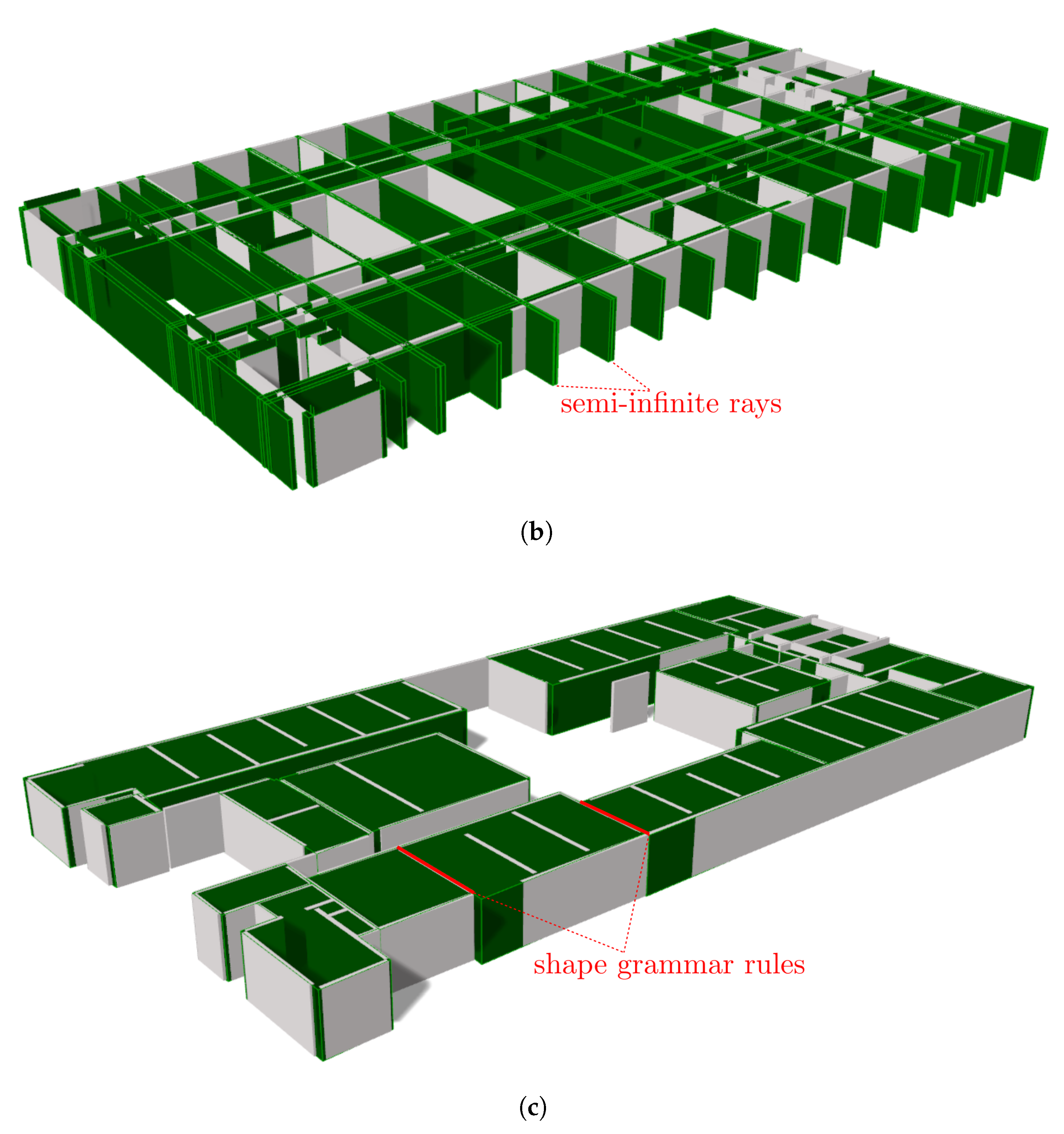
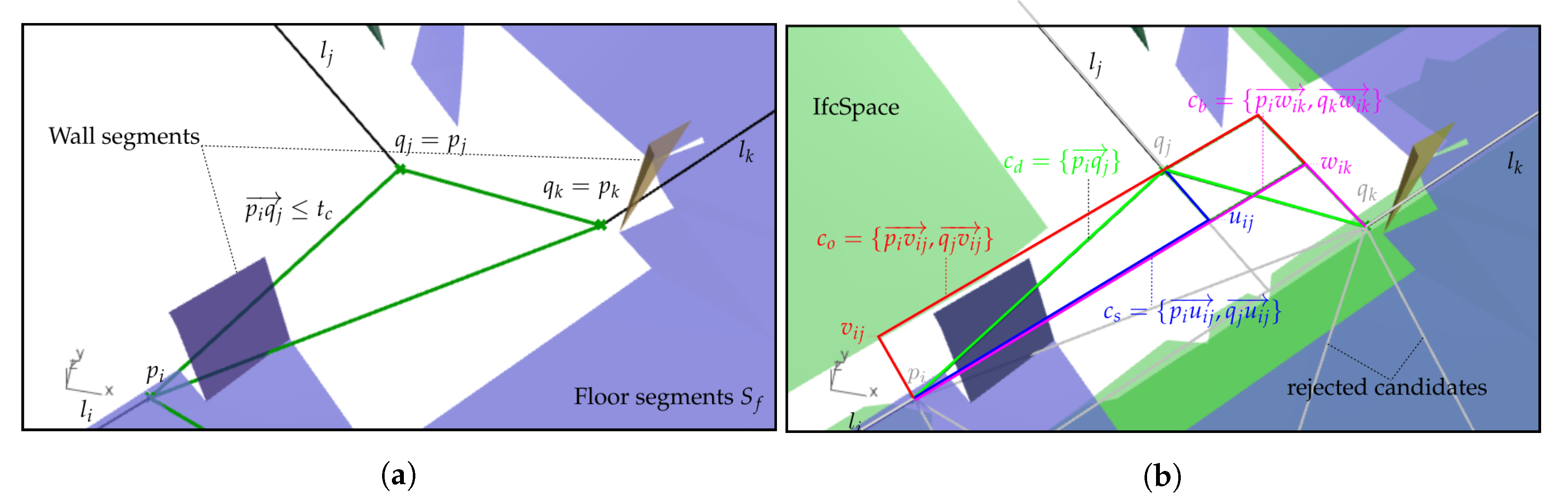
3.3. Candidate Connections

Given $N_i$ and $Q_i$, the four types of connections are established between $p_i$ and every $q_j\in Q_i$ (Equation (2)): the intersection between the wall axes $l_i$ and $l_j$ (Figure 4a), the intersection between the normals $\overrightarrow{n\left(p_i\right)}$ and $\overrightarrow{n\left(q_j\right)}$ at respectively $p_i$ and $q_j$ (Figure 4b), the combination of both (Figure 4c) and finally also the direct connection with the shortest Euclidean distance $\overrightarrow{p_i{q}_j}$ (Figure 4d).

$$\begin{array}{cc}\hfill & U_i=\left\{u_{ij}|\forall l_j\in N_i:u_{ij}=l_i\cap l_j\right\}\hfill \\ \hfill & V_i=\left\{v_{ij}|\forall q_j\in Q_i:v_{ij}=\overrightarrow{n\left(p_i\right)}\cap \overrightarrow{n\left(q_j\right)}\right\}\hfill \\ \hfill & W_i=\left\{w_{ij}|\forall l_j\in N_i,\forall q_j\in Q_i:w_{ij}=\left\{l_i\cap \overrightarrow{n\left(q_j\right)},l_j\cap \overrightarrow{n\left(p_i\right)}\right\}\right\}\hfill \end{array}$$

(2)

where $U_i$, $V_i$ and $W_i$ are the intersection points of respectively the functions themselves, their normals at $p_i$ and $q_j$ and their combinations. We combine the connections in an upperstrict manner so that the extension of $l_i$ can also intersect with the normal of $l_j$ and vice versa. The result is a set of vector pairs $c\in C_i$ between $p_i$ and its neighboring wall axes (Equation (3)).

$$c\in C_i=\left\{\begin{array}{cc}\mathrm{Intersecting}\mathrm{connection}:\hfill & c_s=\left\{\overrightarrow{p_i{u}_{ij}},\overrightarrow{q_j{u}_{ij}}\right\}\hfill \\ \mathrm{Orthogonal}\mathrm{connection}:\hfill & c_o=\left\{\overrightarrow{p_i{v}_{ij}},\overrightarrow{q_j{v}_{ij}}\right\}\hfill \\ \mathrm{Blended}\mathrm{connection}:\hfill & c_b=\left\{\overrightarrow{p_i{w}_{ij}},\overrightarrow{q_j{w}_{ij}}\right\}\hfill \\ \mathrm{Direct}\mathrm{connection}:\hfill & c_d=\left\{\overrightarrow{p_i{q}_j}\right\}\hfill \end{array}\right.$$

(3)

where the first component of each vector pair ($\overrightarrow{p_i{u}_{ij}}$, $\overrightarrow{p_i{v}_{ij}}$, $\overrightarrow{p_i{w}_{ij}}$ and $\overrightarrow{p_i{q}_j}$) are vectors that connect $l_i$ directly to $l_j$ or to an intersection point in between them. The second component of each vector pair ($\overrightarrow{q_j{u}_{ij}}$, $\overrightarrow{q_j{v}_{ij}}$ and $\overrightarrow{q_j{w}_{ij}}$) connects $l_j$ to the same intersection point. It is important to notice that blended connections are mutually exclusive with intersecting and orthogonal connections. To increase the method’s detection rate, the vector pairs are conditioned not to intersect, within a certain threshold, with IfcSpace geometries R that are temporarily constructed from the 3D convex hull of ceiling segments and their underlying floor segments. Also, the vector pairs may not intersect with wall mesh segments ${\mathbf{S}}_{\mathbf{W}}$ that are directly derived from the point cloud. Finally, the combined length of the vector pair $c\le t_d$. Orthogonal vector pairs are conditioned with a more strict threshold $\alpha t_d$ as a wall axis can be more reliably extended than orthogonally connected (Equation (4)).

$$\begin{array}{cc}\hfill & C_i^{\prime }=\{c\in C_i|\parallel c\parallel =\parallel c_1\parallel +\parallel c_2\parallel :\parallel c\parallel \le t_d\wedge \hfill \\ \hfill & \parallel c_o\parallel \le \alpha t_d\wedge \mathrm{Intersect}(c,{\mathbf{S}}_{\mathbf{W}},R)=\varnothing \}\hfill \end{array}$$

(4)

where $C_i^{\prime }$ is the set of conditioned connections for each $p_i$ to $Q_i$. The length of $c=\parallel c\parallel$ is set equal to the sum of its vector pair. $c_o$ are the orthogonal vector pairs and $\alpha$ is the factor governing the orthogonal distance threshold relative to the intersection threshold $t_d$. The result is a set of valid connections of which only 1 type can be chosen.

3.4. Candidate Selection

For every $C_i^{\prime }$ defined by $\mathbf{P}$, the best suited connection $c_i$ to one of its $Q_i$ is determined by minimizing the extrapolation of the wall axes that is not supported by observations (Figure 3c). As such we define a cost function based on the connection’s length and type (Equation (5)).

$$\begin{array}{cc}\hfill & C=\left\{c_i\in C_i^{\prime }|\forall p_i\in \mathbf{P}:c_i=argmi{n}_{c\in C_i^{\prime }}\left(\frac{\parallel c\parallel }{{\omega }_c}\right)\right\}\hfill \\ \hfill & C^{\prime }=\left\{c_i,c_j\in C|c_i\cup c_j\right\}\hfill \end{array}$$

(5)

where the weight of each connection type ${\omega }_c=\{{\omega }_i,{\omega }_o,{\omega }_b,{\omega }_d\}$ is either set to a default value based on the topology of a manually conceived model of a reference dataset, or by the user as it can be application dependent. In general, the order of the connections (i.e., the order of decreasing weight) is regular intersections, blended connections, orthogonal connections and finally the direct connections. The resulting set $C^{\prime }$ is conditioned to only contain distinct and non-overlapping members to respect the topology of the structure.

3.5. Wall Adjustment

Given $C^{\prime }$, a set of new IfcWallStandardCase objects $W^{\prime }$ is created with the wall parameters of respectively $w_i$ and $w_j$ (Figure 3d). The wall axes (selected from $C^{\prime }$), the base/top constraint $h_{base}$/$h_{top}$ and the walltype $\tau$ of each wall is thus defined as follows (Equation (6)).

$$W^{\prime }=\left\{\begin{array}{cc}\mathrm{I}:\hfill & w_s=\left\{w(\overrightarrow{p_i{u}_{ij}},h_{base,i},h_{top,i},{\tau }_i),w(\overrightarrow{q_j{u}_{ij}},h_{base,j},h_{top,j},{\tau }_j)\right\}\hfill \\ \mathrm{O}:\hfill & w_o=\left\{w(\overrightarrow{p_i{v}_{ij}},h_{base,i},h_{top,i},{\tau }_i),w(\overrightarrow{q_j{v}_{ij}},h_{base,j},h_{top,j},{\tau }_j)\right\}\hfill \\ \mathrm{B}:\hfill & w_b=\left\{w(\overrightarrow{p_i{w}_{ij}},h_{base,i},h_{top,i},{\tau }_i),w(\overrightarrow{q_j{w}_{ij}},h_{base,j},h_{top,j},{\tau }_j)\right\}\hfill \\ \mathrm{D}:\hfill & w_d=\left\{w(\overrightarrow{p_i{q}_j},h_{base,i},h_{top,i},{\tau }_i)\right\}\hfill \end{array}\right.$$

(6)

where the direct connections inherit the parameters of $l_i$ rather than $l_j$. The result of the topology reconstruction is an updated set of IfcWallStandardCase objects $W=\{W\cup W^{\prime }\}$ that form a more logical model (Figure 3d). It is important to notice that this procedure can be repeated multiple times to also allow walls to connect to newly created walls.

From the connected walls, IfcRelConnectsElements relationships and the parametric representation of the connections are automatically defined upon exporting the data to the .ifc data format. Additionally, IfcBuilding and IfcProject information is generated upon export to provide the proper inheritance for the objects. We currently do not store the IfcSpace geometry as it serves as a placeholder in our method.

4. Experiments

The algorithm is evaluated on the Stanford 2D-3D-Semantics dataset (2D-3D-S) created by Armeni et al. [37]. In our experiments, we use regions 1, 2, 4 and 6 because these belong to two multi-story buildings: Area 6 is on top of Area 1, and Area 4 on top of Area 2.

Table 1. Combined Areas 1 + 6 and 2 + 4 of the Stanford 2D-3D-Semantics Data set (2D-3D-S) data set. The data specifications and results are shown for both multi-story datasets.

Stanford 2D-3D-S	Dataset 1 (Area 6 and 1)	Dataset 2 (Area 4 and 2)
Input
#Points/#Mesh faces	85,265,271/357,090	90,301,358/563,565
#Wall segments	486	640
#Wall axes	154	176
#Connections	254	215
Topology
#Partial wall axes	154	176
Runtime	2.2 s	3.3 s
# Connections	219	183
% Recall	75.4	78.1
% Precision	91.5	92.8

shows the specifications of each dataset along with the process time for each operation. Each zone is a realistic representation of the type of building that we are looking to reconstruct. The scenes are littered with clutter and objects of no interest and the structure is occluded in many places. In our experiments, we evaluate the algorithm’s performance to update a set of partial wall axes to properly represent the walls of a multi-story building. To this end, the topology of both datasets was manually reconstructed using the same partial walls. The automatically reconstructed connections are compared to the manually created connections and the false positives are visually inspected for both models. Also, we specifically investigate the performance of the topology reconstruction in a variety of realistic wall configurations (including multiple interlocking walls). All experiments were conducted on a normal laptop with an Intel^® Core™ i7-4900MQ CPU @ 2.8 Ghz with 4 cores, 8 threads and 32 GB RAM.

The reconstruction of the topology is conducted with the following parameters, which are set according to common building logic and by observing the training data. The distance threshold is set to $t_c=3m$, equal to the maximum span width over which walls are allowed to connect. This value is determined from observing the manual connections in the first dataset, which revealed that there is a tradeoff between the span width and the number of false positives. The ratio between intersection and orthogonal connection distance $\alpha$ is set to $0.33$. As mentioned above, this is because orthogonal connections are deemed less reliable to span wider gaps. The weights for the scores of the intersections, the orthogonal connections, the blended connections and the direct connections are respectively set to ${\omega }_c=\{{\omega }_s=0.4,{\omega }_o=0.2,{\omega }_b=0.3,{\omega }_d=0.1\}$ based on an empirical study of the manually created connections in dataset 1. It is important to notice that these parameters are made user-accessible so they can be changed on the fly to improve the detection rate.

On average, the wall topology reconstruction computed a solution for dataset 1 (154 walls) and dataset 2 (176 walls) in under 4 s. The ground truth $C^{\prime }$ for dataset 1 (254) and dataset 2 (215) reveal that on average 71% of the wall axes has to be connected on one or both ends, thus showcasing the need for a topology reconstruction method. Our method succeeded in reconstructing 86% of these connections with on average 76.8% recall and 92.2% precision which is very promising despite the clutter in the environment and the complex wall configurations.

Table 2. Detailed topology reconstruction results of interlocking walls in complex scenarios. Partial walls are shown in black, potential connection in green and final connections in red. The green surfaces depict the IfcSpace geometry and the floor segments are shown in purple.

Successful Connections (Lines, Curves, Polylines)
2 walls
3 walls
n walls

shows the potential connections and final results of some more elaborate wall configurations in the dataset. We also added some curved wall axes as this was not initially present in the Stanford dataset. The results show that the correct connections are determined even in complex multi-wall configurations.

Despite the promising connection results, several errors still remain in the model.

Table 3. Erroneous topology reconstruction results of interlocking walls in complex scenarios. Partial walls are shown in black, potential connection in green and final connections in red. The green surfaces depict the IfcSpace geometry and the floor segments are shown in purple.

Erroneous Connections (Lines, Curves, Polylines)
Room intersection
Overshooting wall axes
Segment intersection

showcases erroneous or absent wall connections. The most frequent errors are caused by faulty ceiling or floor meshes. As connections are conditioned to not intersect with the IfcSpace objects based on these geometries, floors or ceilings in the wrong location can obstruct correct connections from being made. The same applies to wall segments as there are inevitably some meshing, classification and clustering errors. This is clearly reflected by the lower recall values compared to the precision values. To mitigate these problems, the user can choose to not incorporate the wall segments and rooms intersection tests to improve the results. However, this might lead to more false positives which is undesirable. Another issue is the overshoot of some partial wall axes. The partial wall geometry is computed up to the extend of the bounding box of the wall segments and thus this is prone to errors in the clustering and classification procedure. As a result, overshooting wall axes can sometimes produce awkward connections. To mitigate this problem, the user can choose to trim the wall axes up to a certain threshold. However, this increases the confusion for potential connections as a portion of a wall axis is missing.

5. Discussion

The presented methodology is an alternative to the 2D and 3D cell decompositions and shape grammar that currently dominate the literature. In this section, we discuss the pros and cons of our method compared the state of the art. First of all, an important difference to the literature is the extent to which is relied upon Manhattan-world scene assumptions to process the remote sensing inputs. Our method is not bound by these assumptions other than that the scene should represent a building in a logical coordinate system. This is an important advantage over the shape grammar methods such as presented by Tran et al. [12] who struggle with more complex scenes. However, we do still rely on the verticality of the walls since we use IfcWallStandardCase objects. A second major difference is the room-based approach, which is common in literature, versus the wall-based approach that we present to complete the structure’s geometry. Both approaches can produce proper wall geometry but room-based approaches might outperform our method in structures with well defined rooms while our method will have the upper hand in more complex scenarios. A third aspect is the combination complexity of the presented method. Cell decompositions are generally bound by a combination complexity of $O\left(\right(n-1)!)$ which does not only introduce more confusion in the decision framework, but can also lead to faulty connections. Current algorithms typically overcome this by only considering the first intersection which is not always the best solution. In contrast, our method only has a combination complexity of $O\left(nk\right)$ with k the number of potential neighbors which is significantly more efficient in larger datasets. Additionally, this allows us to test for multiple types of connections which is essential to reconstructing a more complete BIM model.

In addition to the existing literature, it is important to discuss the limitations of the method. First of all, more complicated wall configurations can have multiple plausible connection solutions of which we prefer intersections and the least intervening connections. This fits well for the majority of the scenes but without actual building knowledge, this is not a certainty. As the algorithm is highly performant (avg. 2.8 s for both buildings), we made the weights of the connections accessible by the user so the weights can be dynamically adjusted to select the best fit connections. A second shortcoming is the method’s dependency on nearby ceilings, floors and walls. The method’s reliability can be compromised in the absence of these geometries. While the prioritization of the intersection connections is generally the correct choice, the reliability of the method decreases since there is no certainty about the connection type in these configurations. We therefore leave the criteria for the adjacency up to the user who can heuristically determine over which distance a wall axis may be extrapolated to connect to a neighboring wall. This is closely linked to the assumption of function continuity for the extrapolation of wall axes. As the distance threshold increases, the extrapolation of functions (especially for arcs and polylines) becomes increasingly unreliable. In the case of severely occluded point clouds of meshes, the user is encouraged to manually validate the connections as they are error prone due to the lack of observations.

Overall, there is high applicability of this method in the field of processing remote sensing inputs. By enriching the raw metric measurements with semantics such as wall information and reconstructing the topology, the data from Lidar or photogrammetric data acquisition system gets ever more intelligent. This in turn supports the data acquisition itself as prior information has proven to lead to more successful data acquisition procedures for buildings and other structures. For instance, techniques such as next-best-scan [38] and occupancy grid mapping for navigation [39] highly benefit from building topology, enclosed spaces and the whereabouts of certain objects. As such, the future works should include the feedback of the BIM information back to the data acquisition systems.

6. Conclusions and Future Work

This paper presents a novel framework to create a logical BIM model in an unsupervised manner. The method enriches preprocessed remote sensing inputs with the topology of Building Information Modeling conform the IFC standard. The goal of the research is to compute a more complete parametric object representation from the raw point clouds of existing buildings that do not have a preexisting BIM. The presented procedure is the second step in a two-step process that classifies the point clouds, assign a parametric geometry to them in an unsupervised manner and afterwards adjusts these entities to reconstruct the topology. The main contributions of this method are its flexibility to deal with multiple IfcWallStandardCase definitions i.e., straight, curved and polyline-based walls, the multiple types of connection candidates that are considered and its ability to process multi-story buildings.

The method is tested on the Stanford 2D-3D-Semantics dataset (2D-3D-S). Areas 1 + 6 and Area 2 + 4 were successfully reconstructed and topologically adjusted using the proposed method. The detailed analysis of the computed connections reveals that the method is indeed capable of creating proper wall geometry in an unsupervised manner of various complex wall configurations. The experiments indicate that the used method is a promising topology reconstruction framework and has several functionalities that extend the current state of the art. The proposed wall adjustments are similar to what human modelers would prefer and the method deals with complex curves and configurations which can significantly speed up the manual modeling process. While this is a promising result, several issues still remain. In zones with limited observations and where manual modelers also struggle, the method underperforms. Also, walls that do not comply with the IfcWallStandardCase (wall axes) definition are error prone. A manual operator should therefore still validate the model and some manual adjustments may be in order to complete the BIM.

In future work, we will look to expand the applicability of the research. First off all, we will look to integrate a feedback loop to further improve the enrichment of remote sensing inputs. Also, we will strengthen our approach by comparing it to closely related works such as Ochmann et al. [13], Tran et al. [12] and Nikoohemat et al. [14]. Once the wall geometry is established, openings can be detected for the integration of window and door frames. A possible extension towards non-uniform thickness walls is the detection of voids during the wall reconstruction. This detection resembles opening detection and can be used to reconstruct the walls more accurately.

References

1. Taneja, S.; Akinci, B.; Garrett, J.H.; Soibelman, L. Algorithms for automated generation of navigation models from building information models to support indoor map-matching. Autom. Constr. 2016, 61. [Google Scholar] [CrossRef] [Green Version]
2. Díaz-Vilariño, L.; Verbree, E.; Zlatanova, S.; Diakité, A. Indoor modelling from SLAM-based laser scanner: Door detection to envelope reconstruction. In Proceedings of the International Archives of the Photogrammetry, Remote Sensing and Spatial Information Sciences—ISPRS Archives, Wuhan, China, 18–22 September 2017; Volume 42. [Google Scholar] [CrossRef] [Green Version]
3. Volk, R.; Stengel, J.; Schultmann, F. Building Information Modeling (BIM) for existing buildings—Literature review and future needs. Autom. Constr. 2014, 38, 109–127. [Google Scholar] [CrossRef] [Green Version]
4. Hajian, H.; Becerik-Gerber, B. Scan to BIM: Factors affecting operational and computational errors and productivity loss. In Proceedings of the 27th International Symposium on Automation and Robotics in Construction, Bratislava, Slovakia, 25–27 June 2010; pp. 265–272. [Google Scholar]
5. Patraucean, V.; Armeni, I.; Nahangi, M.; Yeung, J.; Brilakis, I.; Haas, C. State of research in automatic as-built modelling. Adv. Eng. Inform. 2015, 29, 162–171. [Google Scholar] [CrossRef] [Green Version]
6. Ma, Z.; Liu, S. A review of 3D reconstruction techniques in civil engineering and their applications. Adv. Eng. Inform. 2018. [Google Scholar] [CrossRef]
7. buildingSMART International Ltd. Industry Foundation Classes Release 4 (IFC4); buildingSMART International Ltd.: Kings Langley, UK, 2020. [Google Scholar]
8. Son, H.; Kim, C. Semantic as-built 3D modeling of structural elements of buildings based on local concavity and convexity. Adv. Eng. Inform. 2017, 34. [Google Scholar] [CrossRef]
9. Oesau, S.; Lafarge, F.; Alliez, P. Indoor scene reconstruction using feature sensitive primitive extraction and graph-cut. ISPRS J. Photogramm. Remote Sens. 2014, 90, 68–82. [Google Scholar] [CrossRef] [Green Version]
10. Mura, C.; Mattausch, O.; Pajarola, R. Piecewise-planar Reconstruction of Multi-room Interiors with Arbitrary Wall Arrangements. Comput. Graph. Forum 2016, 35, 179–188. [Google Scholar] [CrossRef]
11. Becker, S.; Peter, M.; Fritsch, D. Grammar-Supported 3D Indoor Reconstruction From Point Clouds for “As-Built” Bim. ISPRS Ann. Photogramm. Remote Sens. Spatial Inform. Sci. 2015, II-3/W4, 17–24. [Google Scholar] [CrossRef] [Green Version]
12. Tran, H.; Khoshelham, K.; Kealy, A. Geometric comparison and quality evaluation of 3D models of indoor environments. ISPRS J. Photogramm. Remote Sens. 2019, 149, 29–39. [Google Scholar] [CrossRef]
13. Ochmann, S.; Vock, R.; Klein, R. Automatic reconstruction of fully volumetric 3D building models from oriented point clouds. ISPRS J. Photogramm. Remote Sens. 2019, 151, 251–262. [Google Scholar] [CrossRef] [Green Version]
14. Nikoohemat, S.; Diakité, A.A.; Zlatanova, S.; Vosselman, G. Indoor 3D reconstruction from point clouds for optimal routing in complex buildings to support disaster management. Autom. Constr. 2020, 113, 103109. [Google Scholar] [CrossRef]
15. Tran, H.; Khoshelham, K. Procedural reconstruction of 3D indoor models from lidar data using reversible jump Markov Chain Monte Carlo. Remote Sens. 2020, 12, 838. [Google Scholar] [CrossRef] [Green Version]
16. Bassier, M.; Bonduel, M.; Van Genechten, B.; Vergauwen, M. Octree-Based Region Growing and Conditional Random Fields. In Proceedings of the 2017 5th International Workshop LowCost 3D—Sensors, Algorithms, Applications: The International Archives of the Photogrammetry, Remote Sensing and Spatial Information Sciences, Hamburg, Germany, 28–29 November 2017; Volume XLII-2/W8, pp. 25–30. [Google Scholar] [CrossRef] [Green Version]
17. Bassier, M.; Van Genechten, B.; Vergauwen, M. Classification of sensor independent point cloud data of building objects using random forests. J. Build. Eng. 2018, i, 1–10. [Google Scholar] [CrossRef]
18. Previtali, M.; Scaioni, M.; Barazzetti, L.; Brumana, R. A flexible methodology for outdoor/indoor building reconstruction from occluded point clouds. In Proceedings of the ISPRS Annals of the Photogrammetry, Remote Sensing and Spatial Information Sciences, Zurich, Switzerland, 5–7 September 2014; Volume II-3, pp. 119–126. [Google Scholar] [CrossRef] [Green Version]
19. Previtali, M.; Díaz-Vilariño, L.; Scaioni, M. Indoor building reconstruction from occluded point clouds using graph-cut and ray-tracing. Appl. Sci. (Switzerland) 2018, 8, 1529. [Google Scholar] [CrossRef] [Green Version]
20. Jung, J.; Stachniss, C.; Ju, S.; Heo, J. Automated 3D volumetric reconstruction of multiple-room building interiors for as-built BIM. Adv. Eng. Inform. 2018, 2018. [Google Scholar] [CrossRef]
21. Thomson, C.; Boehm, J. Automatic geometry generation from point clouds for BIM. Remote Sens. 2015, 7, 11753–11775. [Google Scholar] [CrossRef] [Green Version]
22. Ambrus, R.; Claici, S.; Wendt, A. Automatic Room Segmentation From Unstructured 3-D Data of Indoor Environments. IEEE Robot. Autom. Lett. 2017, 2, 749–756. [Google Scholar] [CrossRef]
23. Liu, C.; Wu, J.; Furukawa, Y. FloorNet: A unified framework for floorplan reconstruction from 3D scans. In Lecture Notes in Computer Science (Including Subseries Lecture Notes in Artificial Intelligence and Lecture Notes in Bioinformatics); Springer: Berlin/Heidelberg, Germany, 2018; Volume 11210 LNCS, pp. 203–219. [Google Scholar] [CrossRef] [Green Version]
24. Turner, E.; Zakhor, A. Floor Plan Generation and Room Labeling of Indoor Environments from Laser Range Data. In Proceedings of the GRAPP, International Joint Conference on Computer Vision, Imaging and Computer Graphics Theory and Applications, Lisbon, Portugal, 5–8 January 2014; pp. 1–12. [Google Scholar] [CrossRef] [Green Version]
25. Budroni, A.; Boehm, J. Automated 3D Reconstruction of Interiors from Point Clouds. Int. J. Archit. Comput. 2010, 08, 55–74. [Google Scholar] [CrossRef]
26. Wang, R.; Xie, L.; Chen, D. Modeling indoor spaces using decomposition and reconstruction of structural elements. Photogramm. Eng. Remote Sens. 2017, 83, 827–841. [Google Scholar] [CrossRef]
27. Mura, C.; Mattausch, O.; Jaspe Villanueva, A.; Gobbetti, E.; Pajarola, R. Automatic room detection and reconstruction in cluttered indoor environments with complex room layouts. Comput. Graph. 2014, 44, 20–32. [Google Scholar] [CrossRef] [Green Version]
28. Xiao, J.; Furukawa, Y. Reconstructing the World’s Museums. Int. J. Comput. Vis. 2014. [Google Scholar] [CrossRef] [Green Version]
29. Valero, E.; Adán, A.; Cerrada, C. Automatic method for building indoor boundary models from dense point clouds collected by laser scanners. Sensors 2012, 12, 16099–16115. [Google Scholar] [CrossRef] [PubMed]
30. Xiong, X.; Adan, A.; Akinci, B.; Huber, D. Automatic creation of semantically rich 3D building models from laser scanner data. Autom. Constr. 2013, 31, 325–337. [Google Scholar] [CrossRef] [Green Version]
31. Murali, S.; Speciale, P.; Oswald, M.R.; Pollefeys, M. Indoor Scan2BIM: Building information models of house interiors. IEEE Int. Conf. Intell. Robot. Syst. 2017, 2017. [Google Scholar] [CrossRef]
32. Khoshelham, K.; Díaz-Vilariño, L. 3D modelling of interior spaces: Learning the language of indoor architecture. In Proceedings of the International Archives of the Photogrammetry, Remote Sensing and Spatial Information Sciences, Riva del Garda, Italy, 23–25 June 2014; Volume 40, pp. 321–326. [Google Scholar] [CrossRef] [Green Version]
33. Ikehata, S.; Yang, H.; Furukawa, Y. Structured Indoor Modeling. In Proceedings of the IEEE International Conference on Computer Vision, Santiago, Chile, 7–13 December 2015; p. 1540012. [Google Scholar] [CrossRef]
34. Tran, H.; Khoshelham, K.; Kealy, A.; Díaz-Vilariño, L. Shape Grammar Approach to 3D Modeling of Indoor Environments Using Point Clouds. J. Comput. Civ. Eng. 2019, 33. [Google Scholar] [CrossRef]
35. Tran, H.; Khoshelham, K.; Kealy, A.; Díaz-Vilariño, L. Extracting Topological Relations Between Indoor Spaces From Point Clouds. In Proceeding of the ISPRS Annals of the Photogrammetry, Remote Sensing and Spatial Information Sciences, Wuhan, China, 18–22 September 2017; Volume 2017. [Google Scholar] [CrossRef] [Green Version]
36. Bassier, M.; Yousefzadeh, M.; Vergauwen, M. Comparison of 2d and 3d wall reconstruction algorithms from point cloud data for as-built bim. J. Inf. Technol. Constr. 2020, 25, 173–192. [Google Scholar] [CrossRef]
37. Armeni, I.; Sener, O.; Zamir, A.R.; Jiang, H.; Brilakis, I.; Fischer, M.; Savarese, S. 3D Semantic Parsing of Large-Scale Indoor Spaces. In Proceedings of the IEEE Computer Society Conference on Computer Vision and Pattern Recognition, Las Vegas, NV, USA, 26 June–1 July 2016; Volume 2016, pp. 1–10. [Google Scholar] [CrossRef]
38. Prieto, S.A.; Quintana, B.; Adán, A.; Vázquez, A.S. As-is building-structure reconstruction from a probabilistic next best scan approach. Robot. Auton. Syst. 2017, 94. [Google Scholar] [CrossRef]
39. Xu, L.; Feng, C.; Kamat, V.R.; Menassa, C.C. An Occupancy Grid Mapping enhanced visual SLAM for real-time locating applications in indoor GPS-denied environments. Autom. Constr. 2019, 104. [Google Scholar] [CrossRef]
Figure 1. Overview of the Scan-to-BIM procedure from remote sensing point clouds. (a) Point cloud data (b) Extracted building components (c) Geometry reconstruction in occluded areas (d) BIM topology reconstruction.
Remotesensing 12 01800 g001
Figure 2. Schematic overview of the potential methods in the literature to reconstruct building topology (2D-3D-S Stanford dataset). The partial walls are shown in grey while the geometries supporting the reconstruction are shown in green. (a) Overview cell decomposition such as presented by Ambrus et al. [22], Ochmann et al. [13] and Mura et al. [10]. A set of semi-infinite rays (green) is computed from the partial walls (grey) to subdivide the space into cells that are the base geometry for the topology reconstruction. (b) Overview connection evaluations such as presented by Nikoohemat et al. [14] and ourselves. A set of connections (green) is proposed for each set of neighboring partials walls (grey) for the topology reconstruction. (c) Overview shape grammar such as presented by Tran et al. [12]. Given a set of rooms (green), a set of connectivity relations (red) such as containment and adjacency is defined between the geometries to reconstruct the topology.
Remotesensing 12 01800 g002aRemotesensing 12 01800 g002b
Figure 3. Wall topology reconstruction procedure of 3 interlocking walls. The reoccurring elements in each figure are the partial wall axes L = { l i , l j , l k } (black), their wall segments and the floor segments (purple). (a) Neighborhood selection (b) Candidate connections (c) Candidate selection (d) Wall reconstruction.
Remotesensing 12 01800 g003aRemotesensing 12 01800 g003b
Figure 4. Potential connections in a configuration with 3 walls. The reoccurring elements in each figure are the partial wall axes L = { l i , l j , l k } (black), their wall segments and the floor segments (purple). (a) Intersecting connection (b) Orthogonal connection (c) Blended connection (d) Direct connection.
Remotesensing 12 01800 g004