Exploring TanDEM-X Interferometric Products for Crop-Type Mapping

Abstract

The application of satellite single-pass interferometric data to crop-type mapping is demonstrated for the first time in this work. A set of nine TanDEM-X dual-pol pairs of images acquired during its science phase, from June to August 2015, is exploited for this purpose. An agricultural site located in Sevilla (Spain), composed of fields of 13 different crop species, is employed for validation. Sets of input features formed by polarimetric and interferometric observables are tested for crop classification, including single-pass coherence and repeat-pass coherence formed by consecutive images. The backscattering coefficient at HH and VV channels and the correlation between channels form the set of polarimetric features employed as a reference set upon which the added value of interferometric coherence is evaluated. The inclusion of single-pass coherence as feature improves by 2% the overall accuracy (OA) with respect to the reference case, reaching 92%. More importantly, in single-pol configurations OA increases by 10% for the HH channel and by 8% for the VV channel, reaching 87% and 88%, respectively. Repeat-pass coherence also improves the classification performance, but with final scores slightly worse than with single-pass coherence. However, it improves the individual performance of the backscattering coefficient by 6–7%. Furthermore, in products evaluated at field level the dual-pol repeat-pass coherence features provide the same score as single-pass coherence features (overall accuracy above 94%). Consequently, the contribution of interferometry, both single-pass and repeat-pass, to crop-type mapping is proved.

1. Introduction

Data acquired by the TanDEM-X mission [1] have been used not only for the generation of a global digital elevation model (DEM) of the Earth’s surface [2], which is its main objective, but for many other scientific purposes, such as forest parameter estimation [3,4], global forest mapping [5], glacier changes monitoring [6], measurement of lava discharge rate in volcanoes [7], and many others. In this work, a different application of these data is investigated: the generation of crop-type maps from time series of TanDEM-X data takes.

Crop classification is one of the earliest applications of satellite remote sensing. It has contributed to the improvement of the agricultural statistics, as well as to the mapping of the areas and production of the world’s major crops. Crop-type maps are exploited for market predictions, insurance claims, payment of subsidies, etc., and also for hydrological and ecological purposes, due to the effect of crops on water demand, use of pesticides, preservation of biodiversity, etc. For instance, the recent integration of satellite data into the mandatory checks of the European Common Agricultural Policy, which is required for the allocation of subsidies targeting specific crops, is another example of the advantages of accurately identifying crop types.

The exploitation of synthetic aperture radar (SAR) data for agricultural applications is based both on the capability of radars to acquire images at any daytime and independently of weather conditions, hence providing consistent time series of data, and on the sensitivity of microwaves to the architecture of crop canopies [8,9]. One of the most successful applications of SAR in agriculture is crop classification based on time series of spaceborne images, which has been proved in many studies [10,11,12]. Regarding the use of series of X-band data for crop-type mapping, the earliest example corresponds to an airborne experiment carried out back in 1988 [13], but most studies exploit data from the TerraSAR-X satellite mission, launched in 2007, and its twin satellite TanDEM-X launched three years later.

To date, time series of dual-pol SAR images acquired by TerraSAR-X and TanDEM-X have been successfully applied for crop classification by exploiting either the backscattering coefficient at the two channels [14,15,16] or sets of polarimetric features [17,18,19,20] as inputs to the classifier. An intercomparison is complicated due to the specific conditions of each experiment, in terms of the crop types present in the study sites and the available sets of images. However, the best reported overall accuracies are around 70–80% when only backscattering coefficient features are employed, and they reach 95% in the best case when also polarimetric features are added and the evaluation is done at field level [19].

This work is aimed at exploring the added value of the interferometric products that can be derived from TanDEM-X data for classification of agricultural crops. For this purpose, two different types of interferometric combinations are investigated: single-pass and repeat-pass. Single-pass interferometry consists in combining two images acquired simultaneously over the same scene, whereas repeat-pass interferometry is the combination of images acquired on different dates by the same satellite. It is important to note that TanDEM-X is a unique radar sensor in space because it is currently the only one providing pairs of images acquired simultaneously by two satellites (TerraSAR-X and TanDEM-X), hence enabling single-pass interferometry, whereas repeat-pass is the common interferometric mode for all radar satellites.

The expected contribution from single-pass interferometric to crop-type mapping relies on the sensitivity of coherence to the height and structure of the plants, which are attributes specific of each crop species and also evolve with time along the growing season. The use of single-pass interferometric coherence for classification purposes is rather scarce, with only a few examples in the literature, apart from the forest/non-forest global map generated from TanDEM-X data [5]. Interferometric coherence acquired by airborne sensors with negligible temporal decorrelation, i.e., equivalent to single-pass, was used in the past for classifying forest types according to their different structures and heights [21,22,23], for which polarimetry and interferometry were exploited simultaneously. Similarly, a study on urban land cover classification using polarimetric SAR interferometry (PolInSAR) was carried out in [24]. Therefore, to the authors’ knowledge the present study on crop classification is original in the use of this type of data as input features.

As for repeat-pass interferometry, the changes produced in the scene between the acquisition dates generate a decrease in the interferometric coherence known as temporal decorrelation. Provided that these changes are associated with specific crop types and/or at particular dates along the growing cycle, repeat-pass coherence should provide information useful for crop classification. In a broader context, repeat-pass interferometry was tested in the past for land cover mapping by making use of time series of ERS tandem data [25,26], with 1 day revisit time, and more recently with Sentinel-1 data [27,28], with 6 days revisit time. The revisit time of the TanDEM-X mission is 11 days, so areas with vegetation are expected to decorrelate significantly due to the presence of wind (and other weather events) and also due to the changes in the scene induced by the vegetation itself (e.g., crop growth during vegetative phases). Contrarily, bare surfaces usually keep a high coherence over longer periods. As a result, the absence of vegetation, especially at the beginning of the season and after harvest, is expected to be detected by repeat-pass interferometry over agricultural areas. This detection would provide information related to the crop calendar, which normally depends on the crop type, hence being useful for crop-type mapping [11,12,29,30]. The influence of the wavelength or frequency band on temporal decorrelation is also an important aspect to be considered in this context [31,32]. In general, a shorter wavelength (higher frequency) decorrelates faster than a longer wavelength (lower frequency). Repeat-pass coherence from TerraSAR-X was tested for the first time for crop classification in [18], but results were inconclusive about the contribution of this feature for crop-type mapping. The coherence values reported in that paper are compared to the ones found in this work in Section 3.

In the present work we quantify the added value of interferometric coherence as input feature for crop classification. In order to carry out this measurement, we first consider the use of dual-polarimetric features as the reference case, but the results obtained by individual backscattering coefficient of the two channels are also studied to test whether any improvement is provided by interferometry in the single-pol case or not. Moreover, results are evaluated both at pixel and field levels to check whether the contribution of interferometry depends on the spatial level of the products. In addition, the polarimetric and interferometric data are also evaluated when expressed in the Pauli basis, the most common in PolInSAR, to check the potential benefit of this alternative formulation.

A set of nine TanDEM-X data takes gathered from June to August 2015 over an agricultural area in Spain is analysed. A widely used supervised classification method (random forest) is employed to evaluate different sets of input features and to compare their impact both at global level and for different crop species.

2. Material and Methods

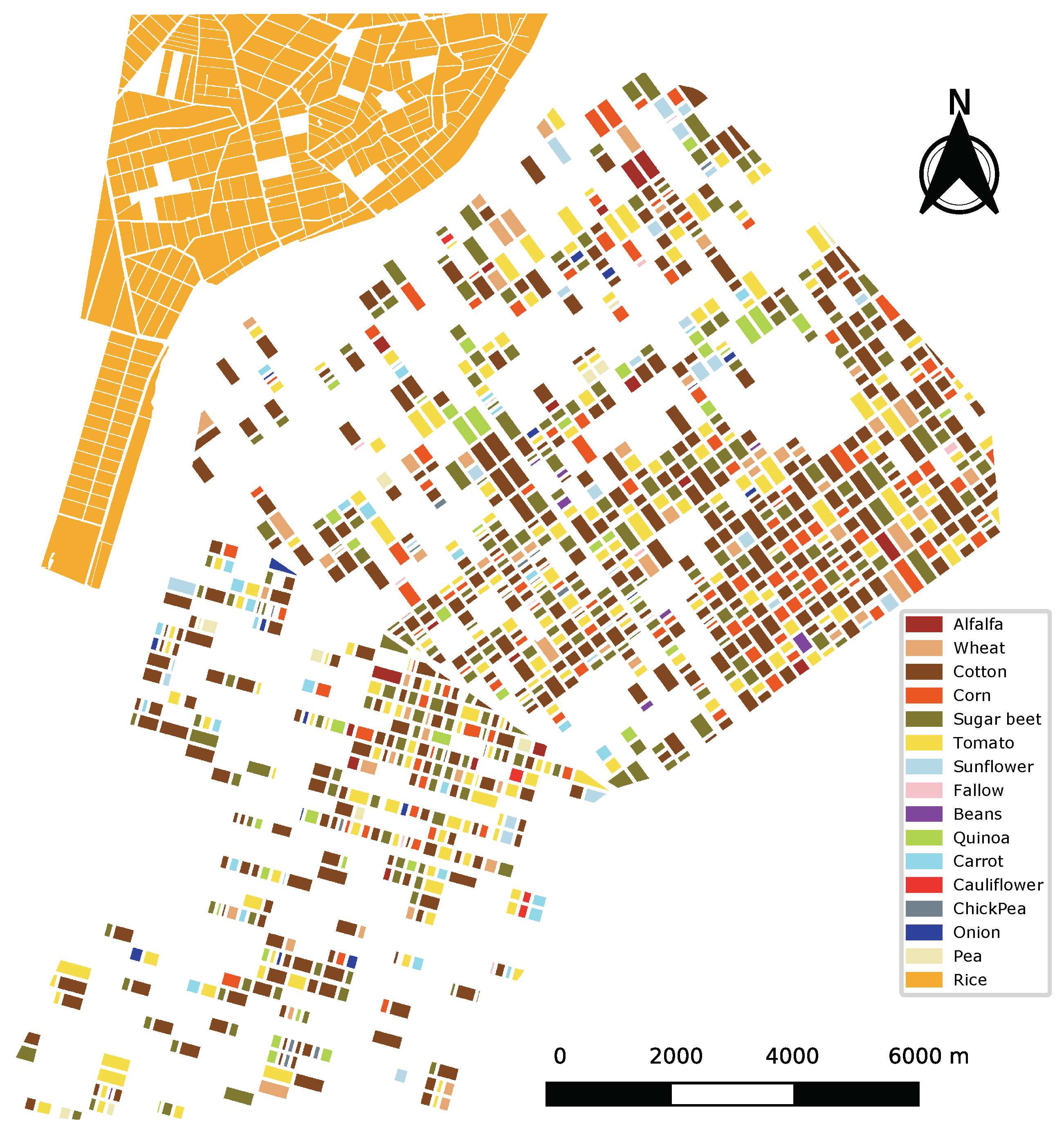
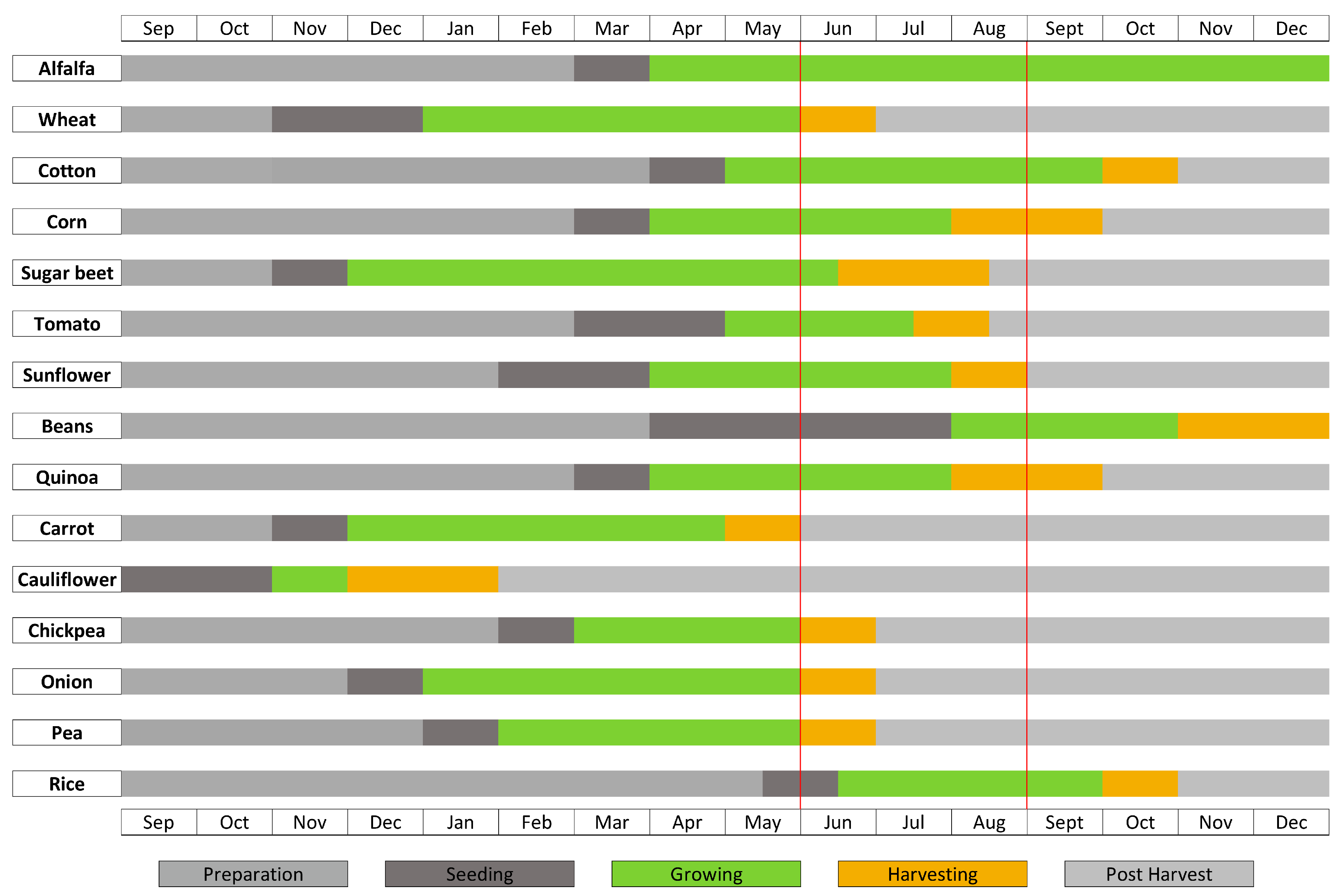
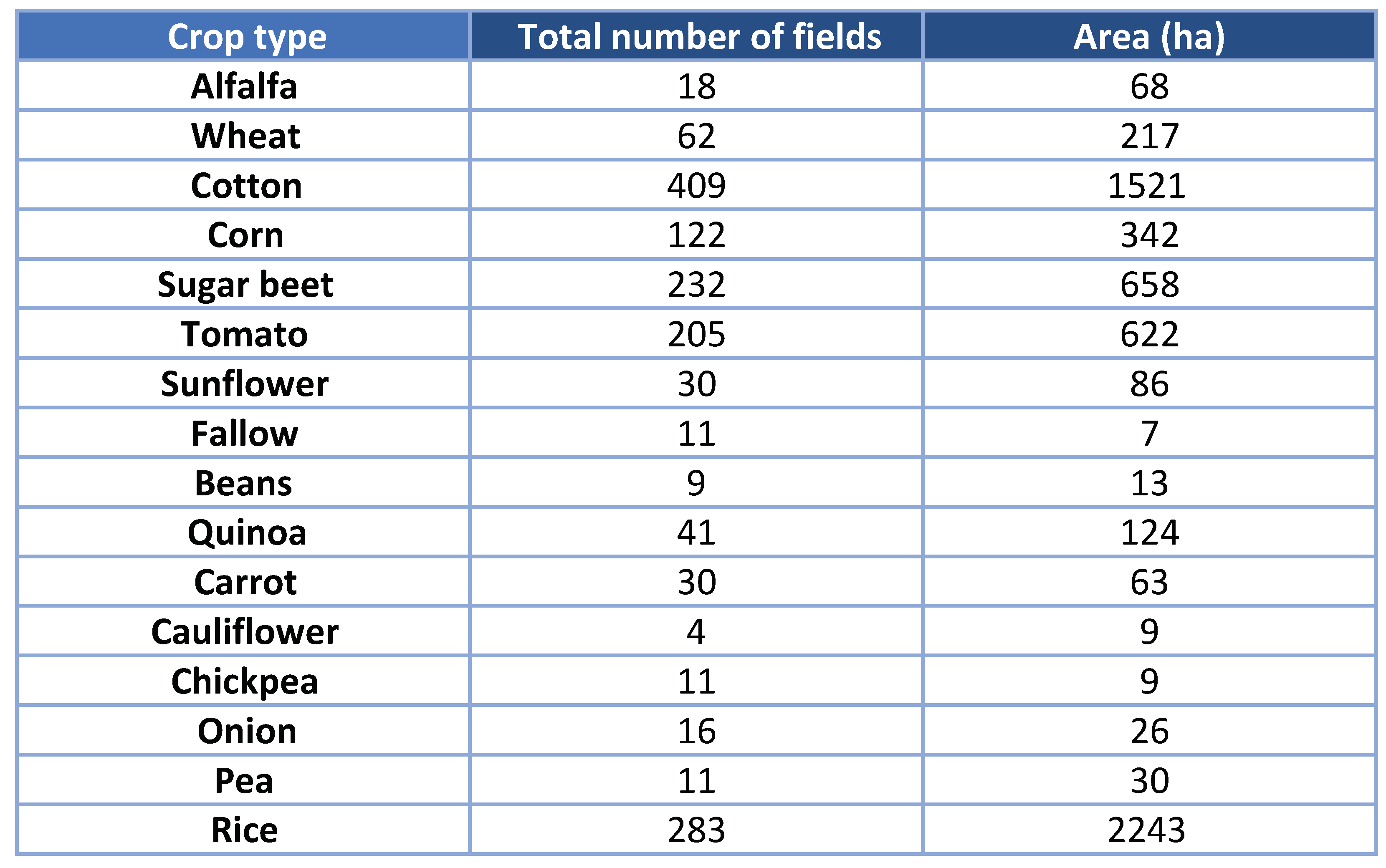
2.1. Reference Data

The study site is located in Sevilla (Spain), centred at 37 N, 6.1 W. It is composed by an agricultural area named BXII Sector, and part of a rice cultivation area. Figure 1 shows the corresponding crop-type map with all fields available in the reference data, which corresponds to the year 2015. During the observation period, from June to August, the weather was very dry and hot in this area, with only two light rain events (less than 2 mm) on June 12 and August 8.

The number of fields per crop and the total area of each crop are summarised in

Table 1. Table of number of fields and total area per crop type in the study site.

. There is a total of 15 crops and some parcels marked as fallow. The dominant crops are rice and cotton, followed by sugar beet, tomato, corn and wheat. All crops are distributed over the whole site except rice, which is only present in the upper left corner.

The crop calendar of all crops in this area is shown in Figure 2. The different stages defined for each crop are ’Preparation’, ‘Seeding’, ‘Growing’, ‘Harvesting’ and ’Post harvest’. The cropping pattern is a diverse mixture representative of most of the field crops and vegetable grown in the Guadalquivir valley. It includes winter (sugar beet, wheat, quinoa) and spring crops (rice, cotton, tomato, corn) whose growth cycles last until the end of spring or the end of summer, with maximum vegetation cover in June–July. It also includes short-cycle vegetables grown during the winter, being carrot the most relevant. All crops but alfalfa are annual crops (i.e., one cultivation per year), whereas the cultivation of alfalfa lasts several years. In the reference data, all the alfalfa fields were sown in 2015.

The two red vertical lines overlaid to the crop calendar define the available period of observation with TanDEM-X data, from beginning of June to end of August, which is detailed in Section 2.2. We can easily appreciate that the satellite data cover only partially the cultivation cycle of the crops, and in some cases the whole life cycle is outside the temporal interval under investigation. Crops like wheat, chickpea, onion and pea are only covered in their harvesting stage, while others like carrot and cauliflower are completely out of the observed period.

Since these two last crops were harvested before the satellite acquisition dates, the radar data do not provide information about them, so both will be removed from the classification dataset. Those crops whose life cycle is only partially covered by the satellite data will be not removed from the dataset, but it is expected that the classification results obtained for them will not be satisfactory. Another land cover class which will be removed is fallow, since it is not really a crop type and may be subject to different practices during the observed period. Consequently, the total number of crops considered in the experiment is 13.

2.2. TanDEM-X Data

TanDEM-X (TerraSAR-X add-on for digital elevation measurement) is the name of TerraSAR-X’s twin satellite, and also the name of the mission flying the two satellites in a closely controlled formation, with typical distances between 250 and 500 m [1]. The SAR instruments operate at a central frequency of 9.6 GHz (3.1 cm wavelength), flying at altitude of 514 km. Images can be acquired with different modes that provide a range of resolutions and coverages. Moreover, both single- and dual-polarimetric modes are standard acquisition modes. The prime objective of this mission is the generation of digital elevation models with global coverage and high accuracy. Beyond that, TanDEM-X provides a highly reconfigurable platform for the demonstration of new SAR techniques and applications.

In the standard acquisition mode of the TanDEM-X mission, one satellite acts as a transmitter and the two of them as receivers, hence producing a monostatic image and a bistatic image over the same scene. These two images are co-registered and delivered in a common product format called coregistered single-look slant-range complex (CoSSC).

The interferometric combination of the two images correspond to single-pass interferometry, for which temporal decorrelation is null. The most relevant term affecting the single-pass interferometric coherence in vegetated areas is the so-called volume decorrelation, which stands for the coherence loss due to the presence of scatterers at different heights inside the resolution cell. In fact, volume decorrelation is the key driver for the estimation of vegetation height from TanDEM-X interferometric coherence, since it depends directly on vegetation height [33,34]. The sensitivity of the coherence to vegetation height and structure is controlled by the height of ambiguity (HoA) of the interferometric configuration. HoA is the height difference that generates a change of $2\pi$ in the interferometric phase, and is inversely proportional to the spatial baseline (separation of the two satellites) at the time of acquisition. In this regard, the typical values of HoA for TanDEM-X during its normal operation are from 30 to 80 m, which are optimised for the global DEM generation. These values are also well suited for forest studies, but they are too large for field crops, since plants are much shorter than trees, and InSAR phase is not sensitive to such a low vegetation. However, during the science phase of TanDEM-X, from April to September 2015, the spatial baseline was increased to 2–3 km, hence providing HoA values of a few meters and, consequently, interferometric sensitivity to short crops.

The list of TanDEM-X CoSSC products employed in this study is shown in

Table 2. List of TanDEM-X data takes (CoSSC products).

Date	Master/Slave	Incidence Angle (Degrees)	HoA (m)
4 June 2015	TDX/TSX	22.71	2.53
15 June 2015	TDX/TSX	22.71	2.53
26 June 2015	TDX/TSX	22.73	2.53
7 July 2015	TDX/TSX	22.73	2.54
18 July 2015	TDX/TSX	22.73	2.53
29 July 2015	TDX/TSX	22.74	2.53
9 August 2015	TDX/TSX	22.73	2.52
20 August 2015	TDX/TSX	22.73	2.53
31 August 2015	TDX/TSX	22.73	2.53

. They were acquired from 4 June to 31 August 2015, i.e., inside the science phase, with an incidence angle around 23 degrees and providing a HoA around 2.5 m. All the images correspond to a dual-pol mode with the two copolar channels: HH and VV. The same dataset was previously used in [35] for the retrieval of rice height by using PolInSAR. The spatial resolution of these CoSSC products is 6.6 m in azimuth and 3.1 m in ground-range, while the pixel spacing (pixel size) is 2.4 m in both coordinates.

For the objective of this work, three different sets of observables, to be used as input features for classification purposes, were computed: polarimetric features (backscattering coefficient and correlation between channels), interferometric coherence in single-pass mode, and interferometric coherence in repeat-pass mode. The processing of the data required for each one of these sets is slightly different, so it is described separately in the following subsections.

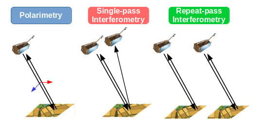
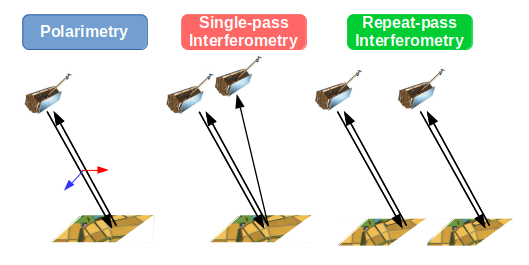
2.2.1. Polarimetric Data

All the single-look complex (SLC) images of the master acquisitions were pre-processed with the following steps: (1) subset of the region of interest, (2) calibration, (3) formation of polarimetric covariance matrices, (4) speckle filtering using a 9 × 9 boxcar filter, (5) computation of observables, and (6) geocoding. The geocoding step, which is common to all observables in this study, was carried out to a common UTM grid with 2 m pixel spacing in both coordinates.

As for the formation of the polarimetric covariance matrix, in the HHVV dual-pol case it results in:

$$\left[C\right]=\left[\begin{array}{cc}|S_{HH}{|}^2& S_{HH}·S_{VV}^{*}\\ S_{VV}·S_{HH}^{*}& |S_{VV}{|}^2\end{array}\right]$$

(1)

where $S_{PP}$ denotes the complex amplitude of the image obtained by transmitting and receiving polarisation $P=\{H,V\}$.

Once $\left[C\right]$ is properly estimated with the speckle filter, the backscattering coefficient values at HH and VV correspond directly to the diagonal entries, $C(1,1)$ and $C(2,2)$, respectively. The normalised complex correlation between the two channels is defined as,

$${\rho }_{HHVV}=\frac{C(1,2)}{\sqrt{C(1,1)·C(2,2)}}$$

(2)

where $|{\rho }_{HHVV}|$ is the correlation (or coherence) between HH and VV, and $arg\left({\rho }_{HHVV}\right)=arg\left(C(1,2)\right)$ is the phase difference between both channels.

From the four features that can be extracted directly from the covariance matrix, we will employ in this study the backscattering coefficient in the two available polarisation channels and the normalised correlation between the two channels, since the performance for crop-type mapping of the phase difference between HH and VV was found to be poor with respect to the other features [20].

In addition to the observables computed directly in the linear basis, i.e., defined for channels HH and VV, some tests are also carried out at the end of this study using two polarimetric channels of the Pauli basis to define all observables. The first Pauli channel corresponds to HH+VV, i.e., the coherent addition of the SLC images at HH and VV channels, whereas the second Pauli channel corresponds to HH-VV, i.e., the subtraction of HH and VV. These two Pauli channels, hereafter denoted as P1 and P2, are easily interpretable in terms of the scattering mechanisms present in the scene [23,33]: P1 is high in presence of surface scattering, whereas P2 is characteristic of double-bounce scattering. Besides an easier interpretation, we showed in [20] that using only the backscattering coefficient of P1 and P2 provided almost the same classification accuracy as the three mentioned features in the linear basis. In addition, the Pauli basis is the most commonly employed in PolInSAR when applied in single-pass mode for studies over vegetated areas [33].

As it is outlined in the Introduction, other polarimetric features could be used as inputs for the classifier, as they have been tested at X band in [17,18,19,20]. However, we have not included them in this work because the main focus is placed on the contribution of the interferometric coherence provided by TanDEM-X, which has not been studied elsewhere.

2.2.2. Single-Pass Interferometric Data

The second set of observables is composed of the single-pass interferometric coherence at the two copolar channels, HH and VV. The CoSSC products provide the master and slave images already coregistered, so the processing steps required in this case were: (1) subset of the region of interest, (2) range spectral filtering, (3) removal of flat Earth and topographic phase components, (4) computation of coherence using a 9 × 9 boxcar filter, and (5) geocoding.

The common range spectral filtering is required to compensate for the geometrical or baseline decorrelation, due to the different incidence angle in the master and slave images. This term is specially important for data acquired during the science phase of TanDEM-X, since the large baseline yields important shifts in the wavenumber, producing values of coherence below 0.8.

After the range filtering we removed the flat Earth and topographic phase terms from the interferograms, so the remaining interferometric phase only contains topographic information with respect to the DEM employed in the processing. The removal of these phase components is also necessary for a good estimation of the coherence, since the presence of phase ramps would decrease it. Finally, the interferometric coherence at both HH and VV channels were computed using a 9 × 9 multi-look filter filter.

2.2.3. Repeat-Pass Interferometric Data

The third set of features corresponds to the repeat-pass interferometric coherence, also at HH and VV channels, obtained by combining images acquired in consecutive passes. In order to obtain coherence estimates, the starting data are the master images present in all CoSSC products, since their original orbital information is available and is equivalent to any conventional TerraSAR-X product. From the nine master images, eight interferometric pairs are formed, as listed in

Table 3. List of repeat-pass interferograms.

Master Date	Slave Date	HoA (m)	Baseline (m)
4 June 2015	15 June 2015	1526	5
15 June 2015	26 June 2015	40	168
26 June 2015	7 Jule 2015	47,730	1
7 July 2015	18 July 2015	450	16
18 July 2015	29 July 2015	69	97
29 July 2015	9 August 2015	101	61
9 August 2015	20 August 2015	164	41
20 August 2015	31 August 2015	127	53

. Compared to the single-pass products, the heights of ambiguity are now much higher thanks to the short spatial baselines produced by the orbits of the satellite.

In this case, the processing steps required to obtain the repeat-pass interferometric coherence were: (1) subset of the region of interest, (2) coregistration of the SLC images, (3) removal of flat Earth and topographic phase components, (4) computation of coherence using a 9 × 9 boxcar filter, and (5) geocoding. The coregistration was carried out first by taking into account the orbital information and using a backgeocoding algorithm. Then, a refinement was applied based in isolated point scatterers. The common band range spectral filtering was applied but it had almost no effect since the spatial baselines were really short, so we have not included it here as a required step.

2.2.4. Interpretation of the Interferometric Coherences

The measured coherence depends on a number of aspects related to the sensor configuration and to the scene properties. In order to interpret this dependence in the observed interferometric coherence and to understand their influence on the crop-type mapping application, coherence can be expressed as a product of decorrelation terms, bounded between 0 and 1, as follows [36,37]:

$$\gamma ={\gamma }_{\mathrm{temp}}·{\gamma }_{\mathrm{geom}}·{\gamma }_{\mathrm{vol}}·{\gamma }_{\mathrm{SNR}}·{\gamma }_{\mathrm{proc}}·{\gamma }_{\mathrm{BAQ}}$$

(3)

where all terms are described next:

• ${\gamma }_{\mathrm{temp}}$ is the temporal decorrelation due to changes in the scene occurred during the acquisition times of both images. In single-pass interferometry this term can be neglected, i.e., ${\gamma }_{\mathrm{temp}}=1$.
• ${\gamma }_{\mathrm{geom}}$ is the decorrelation due to the spatial baseline, also named as geometric decorrelation, which causes a wavenumber shift, i.e., a change in the band occupied by the range coordinate spectrum of both images [38]. This term is cancelled in the pre-processing by filtering the master and slave images to the common frequency band in the range dimension, as it is explained in Section 2.2.2. This filtering entails a loss of spatial resolution in the range coordinate, which may compromise the output product in applications in which very fine resolution needs to be maintained.
• ${\gamma }_{\mathrm{vol}}$ is the coherence due to the vertical distribution of scattering properties of the scene, usually named as volume decorrelation because it is always present whenever there is vegetation volume in the scene.
• ${\gamma }_{\mathrm{SNR}}$ denotes the decorrelation due to thermal noise in the sensor, which depends on the signal-to-noise ratio (SNR) at each pixel. The decorrelation due to SNR can be estimated and compensated as explained in [3,35], but we decided not to compensate it to keep the data processing as simple as possible and because it would be only required in quantitative studies, e.g., vegetation height estimation.
• ${\gamma }_{\mathrm{proc}}$ includes any decorrelation due to the signal processing steps, in which the most important is usually the one due to errors in the coregistration of the images. In our case we consider it is negligible, i.e., ${\gamma }_{\mathrm{proc}}=1$.
• ${\gamma }_{\mathrm{BAQ}}$ is the loss of coherence due to the quantisation of the data with less bits than in the original raw data. Its effect is extensively discussed in [39]. Attending to the 8:3 block adaptive quantisation employed in the products (at both TanDEM-X and TerraSAR-X images) and the type of scene observed (agricultural crops), the average value of decorrelation is around 3.5 %, i.e., ${\gamma }_{\mathrm{BAQ}}\approx 0.965$. This decorrelation term could be compensated for by dividing the measured coherence by this value, but it has not been done in this work because it will not affect the classification performance.

From the definition of these terms it is clear that volume and temporal decorrelation will be the main drivers of the single-pass and repeat-pass coherence, respectively, that will be observed over agricultural crops. This is commented in Section 3 when interpreting the coherence features and the classification results obtained with them.

2.3. Classification Method and Evaluation

Classification was carried out with the random forest (RF) classifier [40] using the implementation provided by the scikit-learn package in python [41,42]. The classifier was run with the default parameters, and they were fixed for all the classification tests described in next section. The required split between training and testing sets was carried out by means of the strategy described in the following paragraph.

First of all, it is important to clarify that due to the spatial filtering employed in the data pre-processing (boxcar of size 9 × 9) the values of the features at every pixel are correlated with those of adjacent pixels. Therefore, to avoid its influence on the classifier, an initial split was performed at field level: for each test, 50% of the fields of each crop type were selected for training and the remaining 50% of the fields were left for testing. Secondly, the strong imbalance in the number of pixels of the crop types present in the scene (proportional to the area shown in Table 1) would affect the classifier by favouring the major classes. To solve this issue, the number of pixels per class finally employed for training was restricted to the lowest value. In other words, the number of pixels of each class used for training was equal for all classes, chosen randomly from the set of available pixels (within the fields initially selected for training) but for the class with least pixels, for which all pixels of the training fields were employed. It must be clarified that the pixels used for training in the classes with least pixels correspond also to half of the total fields (i.e., the initially selected ones), not to the total number of pixels of these classes. This strategy ensures an equitable or balanced training for the random forest algorithm.

For each test, once the training is carried out, the evaluation is carried over the whole set of testing, which is formed by all pixels of the fields initially selected for testing (50% of the total fields). From the results obtained over the pixels in the testing data, the confusion matrix is computed and some metrics are derived [43]: overall accuracy (OA), Kappa coefficient, producer’s accuracy (PA) and user’s accuracy (UA).

Finally, to reduce the potential particularities of the initial split of fields, the whole procedure is repeated 10 times and the final accuracy metrics are averaged. After this number of iterations we observed that the results were stable, with very small variations around the averages.

The classification results are evaluated in two different ways: at pixel level and at field level. In the second case, after the classification is carried out at pixel level, the mode (most frequent value) of the classes present at each field is assigned as the class of that field. Then, the confusion matrix and the derived metrics for assessment are computed from the sets of fields instead of the sets of pixels.

The objective of evaluating the results at both pixel level and field level is two-fold. In first place, from the point of view of the objective of this work, i.e., demonstrating the contribution of TanDEM-X coherence to crop classification, we want to show whether this contribution is consistent or it depends on the spatial level of the classification (pixel-based or field-based). In second place, both levels have their own relevance from the end-user perspective.

In many final applications, a field-based classification map is the typical product, e.g., for agencies and regional institutions which need to check or update their databases. However, the final product of crop classification is not necessarily a parcel map, and therefore the conversion from pixel classes to field classes is not always carried out. For instance, in order to obtain crop acreage statistics (i.e., amount of surface cultivated per crop type) for an irrigation area, a basin, or a county, information at pixel level would suffice. Another example in which pixel information is relevant is when the crop-type maps are used as input data to irrigation or water consumption models. Most of these models work with information in raster format, not with field polygons, so the conversion to parcel maps is not required. Finally, the parcel scale is required mainly for farm management and survey, and it requires an extra work because it needs the parcel maps, e.g., LPIS, which may change from year to year. In many occasions these parcel inventories are not available from one campaign to the next (because they change), hence the conversion from the pixel-level information to a field-level database demands extra processing (segmentation, filtering, etc.). For all these reasons, it is convenient to evaluate both types of results.

The methodology explained in this section is applied in the next section to different sets of input features in order to assess the contribution of the different radar observables provided by TanDEM-X for crop-type mapping.

3. Results

3.1. Inspection of the Features

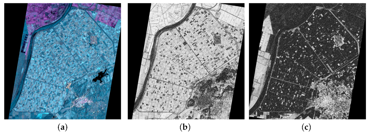
3.1.1. Images of Features

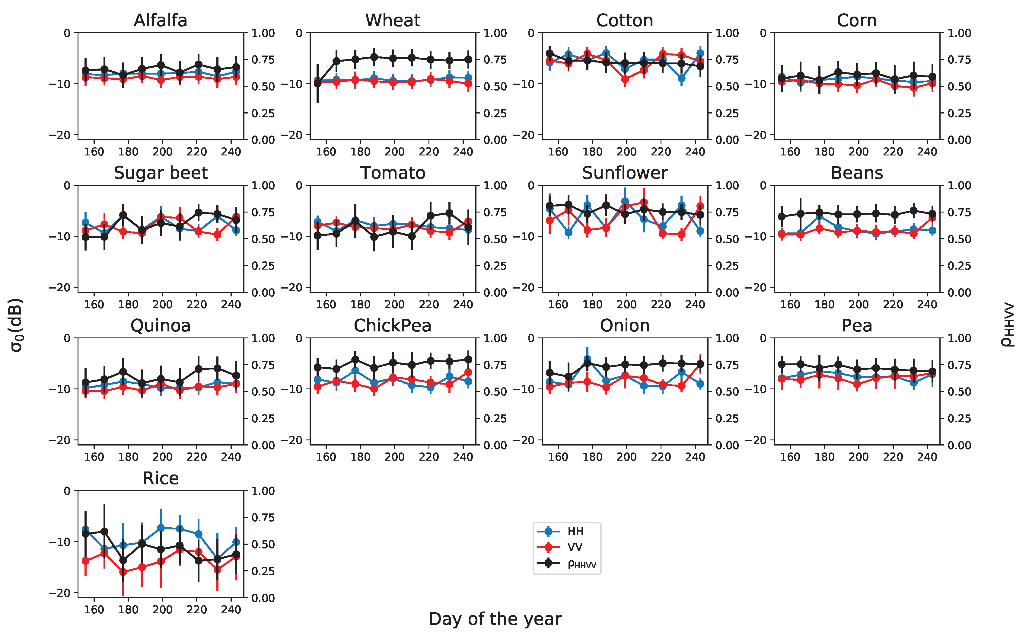
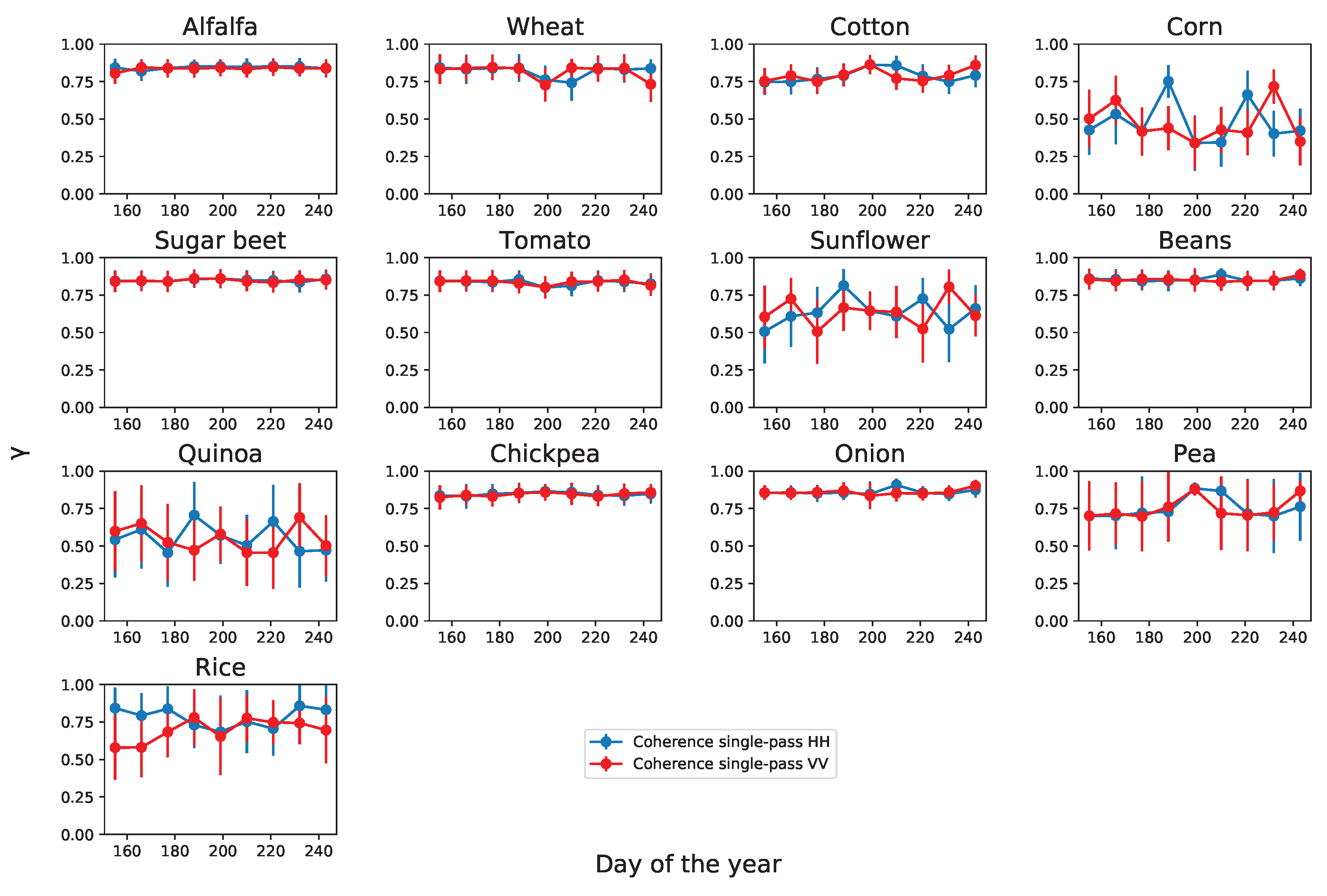
In order to provide a first impression about the radar observables which have been used as input features for the classifier, some of them are represented in Figure 3.

The first image in Figure 3 corresponds to a false colour composite of the backscattering coefficient values at channels VV (green), P1 (blue) and P2 (red), obtained from the image acquired at 7 July 2015. This channel combination is similar to the typical Pauli RGB images, but the cross-polar channel (not available in these data) has been substituted by the VV channel. We can easily identify the rectangles of the agricultural area with different blueish and grey colours, as well as the rice fields in pink colour in the upper part of the site. At the bottom right corner we can easily identify a bright grey area that corresponds to the town of Lebrija. From the point of view of crop classification, the observed colour diversity is a good sign.

The other two images in Figure 3 represent the interferometric coherence at the HH channel obtained at the same date (single-pass coherence shown in Figure 3b) and by combining this date with the next one (repeat-pass coherence shown in Figure 3c). The two coherence values are similar over some areas and different over other locations in the study site, which constitutes an indication of their complementarity.

3.1.2. Time Series

The temporal evolutions of all the radar observables derived from the linear basis (HH, VV), which will be used as input features for classification, are shown in Figure 4, Figure 5 and Figure 6 for all thirteen crop types. For all features, the mean value and standard deviation are computed from all pixels of the same crop type. In first place, the HH and VV backscattering coefficient (in dB) and the normalised correlation between them, defined in (2), are represented in Figure 4 at the nine acquisition dates. The single-pass interferometric coherence of both HH and VV channels is displayed in Figure 5, while the repeat-pass coherence of the same channels is illustrated in Figure 6. For this, the resulting repeat-pass coherence values are represented at the dates of the master acquisitions.

The backscattering coefficient values are quite stable along time for some crop types (e.g., alfalfa and wheat), whereas they show large variations for other crops (e.g., rice, sunflower, cotton, and onion) at least in part of the observation period. The potential causes of change in the radar response along time are multiple: crop growth or development, agricultural practices, and weather events (e.g., rain), from which we can discard weather events due to the stable dry condition maintained along the observation period, as introduced in Section 2.1. In fact, it is important to take into account the cultivation calendar of each crop type, shown in Figure 2, to understand the observed responses. For instance, rice, cotton and sunflower were being cultivated along the whole observation period and show strong variations with time, whereas peas were harvested at the beginning of the observation period, hence showing less changes. However, alfalfa is also being cultivated but, due to its uniform morphology along time, does not exhibit changes in its radar response. Other crops, like corn and quinoa, show only slight changes in their backscattered intensity.

Regarding the normalised correlation between the copolar channels, ${\rho }_{HHVV}$, it is expected to be 1 for bare surfaces (HH and VV arrive in phase because are generated at the same point in the scene), and it would be equal to 1/3 is the scene were formed by an ideal random volume only. The temporal evolutions of this feature (black curves in Figure 4) show a narrow excursion for most crops, with all the values in the interval between 0.6 and 0.75. This can be interpreted as a balanced response from both soil and vegetation volume, which is expected for these data: the steep incidence angle (22.7 degrees) favours the soil contribution, whereas the acquisition frequency (X band) provides a significant backscatter from the aboveground volume even from short crops. The crops with most noticeable changes in the correlation between channels are rice, at all dates, and wheat, sugar beet, and tomato at some specific dates. The radar response of rice at X band, including its polarimetric features and its evolution along the growing season, has been described in previous studies, e.g., [44]. Rice shows a very particular behaviour due to a unique characteristic of its cultivation: the soil is flooded (or saturated by water in the worst case) all along the growing season. Therefore, the response from the ground is dominated by the double-bounce scattering mechanism, and there is no influence of soil roughness or moisture.

The interpretation of the single-pass coherence shown in Figure 5 is provided by the decorrelation sources (see Equation (3)) present in this interferometric configuration. In absence of temporal decorrelation, and thanks to the large baselines available (i.e., short HoA values), volume decorrelation, ${\gamma }_{vol}$, is the dominating decorrelation source [45] and provides sensitivity to vegetation height and structure. Volume decorrelation has been exploited in applications of TanDEM-X for vegetation height retrieval, both in forests [3,34,46,47] and crops [35,48]. As the vegetation height increases, volume scattering effects result in a larger coherence loss, and other structural changes produce also variations in coherence. Besides volume decorrelation, an overall effect of signal-to-noise ratio (SNR) is present in most crops because the noise equivalent sigma zero (NESZ) of TanDEM-X is around −20 dB for these scenes, i.e., around 10 dB below the observed backscattering coefficient (see Figure 4). A 10 dB SNR produces a coherence around 0.9, so we cannot expect coherence values greater than this value, as confirmed by the plots shown in Figure 5. However, the effect of SNR decorrelation is quite homogeneous along time and for most crops, so consequently it is not expected to contribute significantly to crop classification.

The four crop types with higher dynamic range in the single-pass coherence are rice, corn, quinoa and sunflower, all of them characterised by tall plants. Moreover, the main part of the growing period of these crops is included in the observation period, hence favouring the detection of changes in the time series. In these four cases there is also a clear difference between the HH and VV channels at some dates, which suggest their suitability for methods based on PolInSAR data to estimate crop structural variables (e.g., height) [35]. From the classification point of view, the worst scenario corresponds to alfalfa, sugar beet, beans, chickpea, and onions, because they show an almost constant high value of coherence during the whole observation period. A high single-pass coherence is characteristic of a bare surface or a very short crop, so for these five crop types the cause is either the crop calendar (they are harvested or just emerging, hence resembling a bare surface) or the short plant height specific of some crop types.

Regarding the repeat-pass coherence displayed in Figure 6, we expect temporal decorrelation to be the most relevant term affecting the coherence (see Equation (3)). The source of temporal decorrelation over agricultural areas is two-fold: first, vegetation is affected by wind, which changes the position of the scatterers in the plants from the master to the slave acquisition and hence decreases the coherence, and second, crops grow and develop new parts during their cultivation, which changes their shape and size in temporal scales from days to weeks, hence producing important changes that drastically reduce the coherence values. It must be pointed out that the coherence is estimated using a finite spatial filter (9 × 9 boxcar) which is a biased estimator that overestimates more the lower values of coherence than the higher ones [49]. As a result, we cannot obtain coherence estimates below some level (around 0.2 in this case). In this regard, the repeat-pass coherence values reported in [18] for a similar crop classification experiment with TerraSAR-X data were estimated with a much smaller kernel size (not indicated in the manuscript) because their lowest level was 0.4. Consequently, a key part of the dynamic range of the coherence was not available in the features, and hence the coherence features did not demonstrate a consistent contribution to the classification performance in that work.

The inspection of Figure 6 provides some interesting insights which are complementary to the other two sets of observables. For instance, there is no noticeable difference between the two polarimetric channels for any crop type, but for rice during the second half of the observation period. This general coincidence between channels is most likely due to the effect of temporal decorrelation, since it affects equally all the polarisations. Furthermore, we can distinguish different temporal evolutions and trends in the average values for the different crops. Some crops exhibit increasing trends, other ones show decreasing trends, and some of them show changes in the trend along time. Coherence is overall quite low, with only some particular cases over 0.5. The highest values of repeat-pass coherence are observed in wheat after the second date (probably due to the post-harvest bare condition of the fields) and in beans in the five intermediate dates (due the bare surface before the crop starts to grow, since it was sown in June–July). Finally, in most cases there is a large variability (large error bars) at all dates, which means that this observable is noisier than others and, unfortunately, may be of limited use as an input feature for classification purposes.

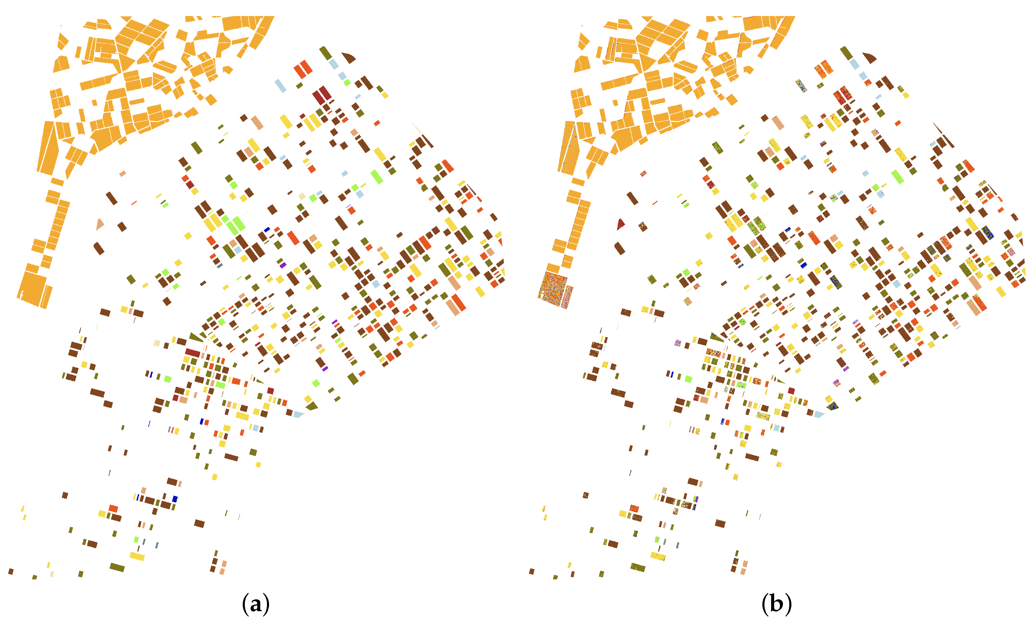
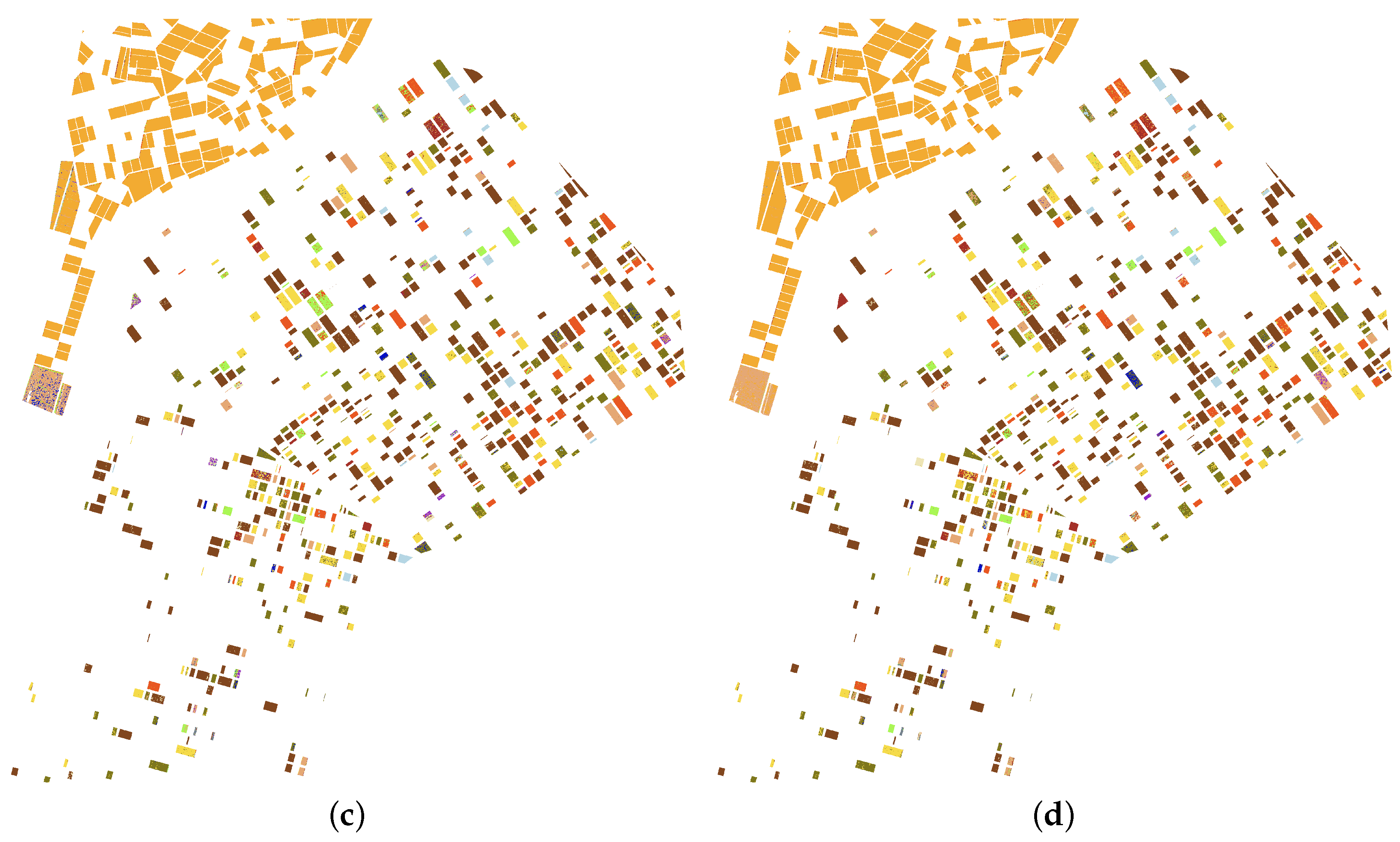
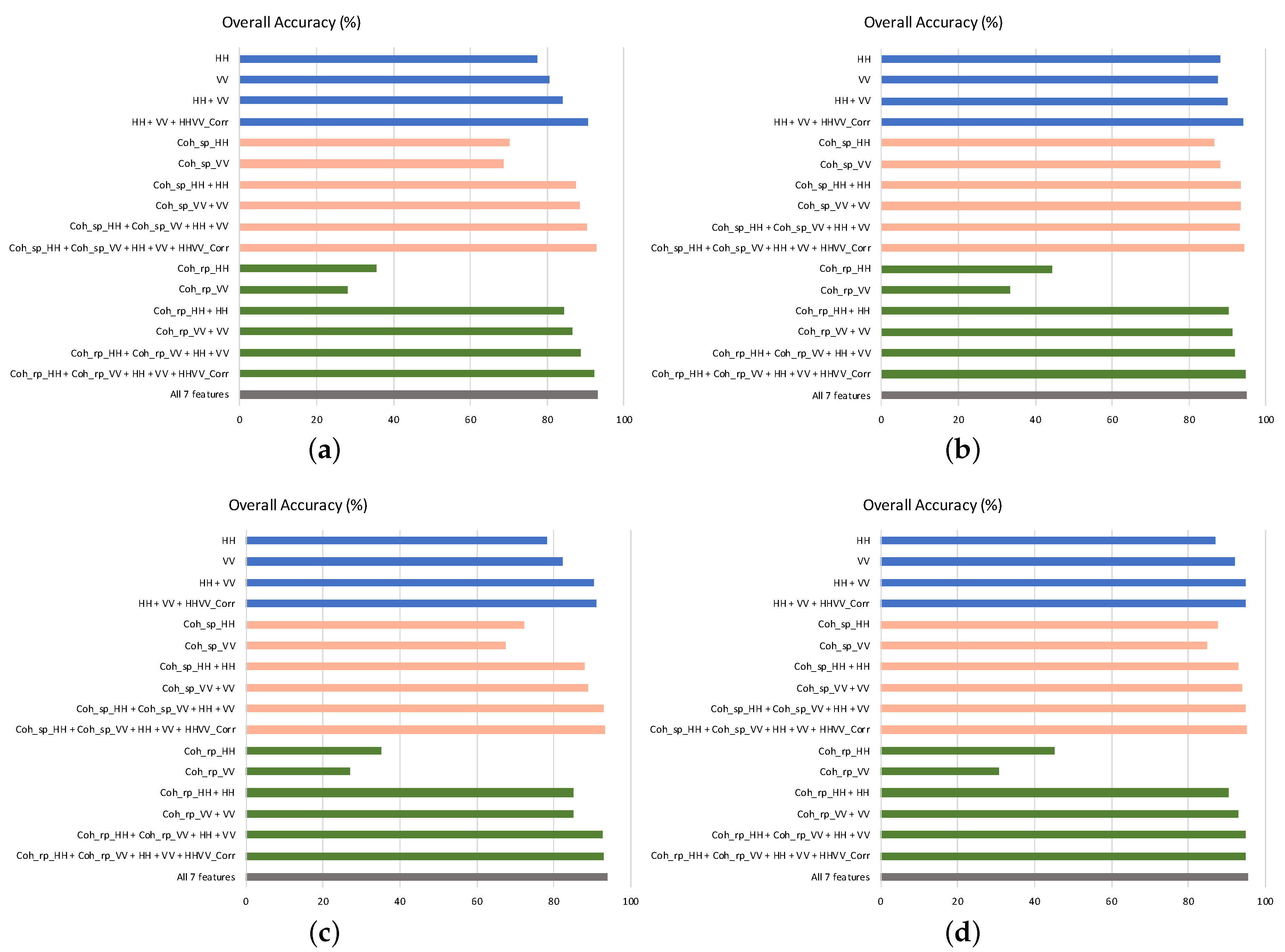
3.2. Classification Results

The analysis of the obtained results is divided into several subsections, which correspond to different sets of input features and to the evaluation at pixel or at field level. In order to simplify the text, the notation employed for all features is the following one:

CC Backscattering coefficient at the CC channel.

CCDD_CorrNormalised correlation between channels CC and DD.

Coh_sp_CCSingle-pass interferometric coherence at the CC channel.

Coh_rp_CCRepeat-pass interferometric coherence at the CC channel.

where CC and DD correspond to HH, VV, P1 or P2, which are defined in Section 2.2.1.

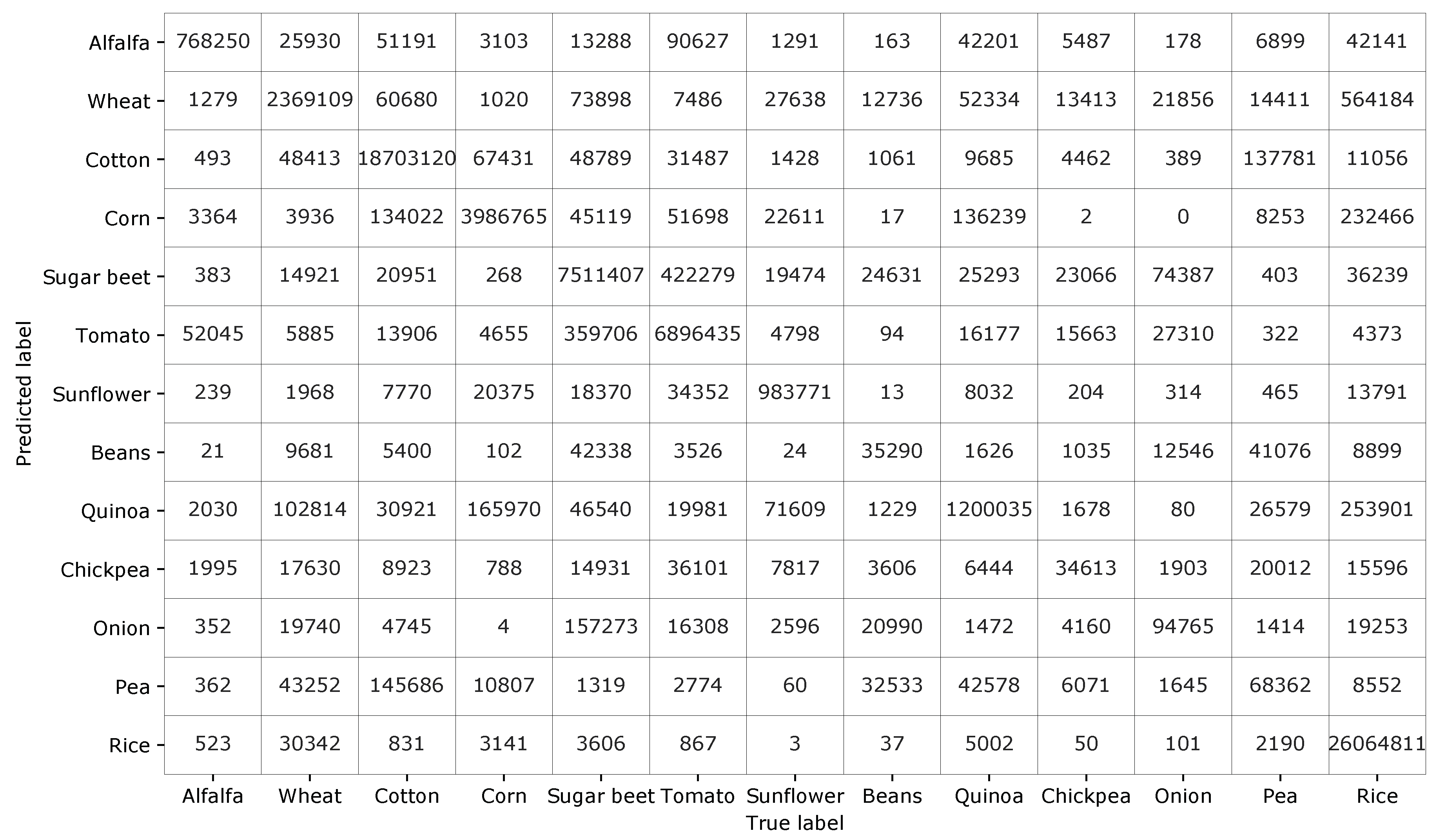
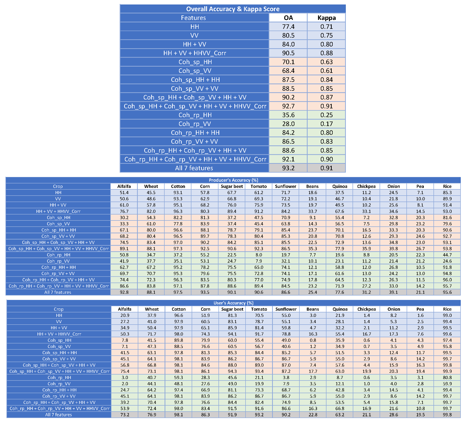
3.2.1. Results at Pixel Level with HH and VV Channels

To begin with, the classification results obtained at pixel level with HH and VV channels are illustrated in

Table 4. Classification scores at pixel level with HH and VV channels. Shading colour: blue for polarimetric features, pink for single-pass interferometric coherence features, green for repeat-pass interferometric coherence features, and grey for all features.

. As it will be done in the rest of the cases, we have divided all the results into 3 different sub-tables. The first sub-table shows the general assessment of the results, hence showing the OA and the Kappa score. Then, the second and third sub-tables show the PA and UA of each crop type, respectively, which provides detailed information about the performance of the classification for each crop type.

Each row in the tables corresponds to a different set of input features. To facilitate the reading of the tables, each one is subdivided in four groups of rows, each group shaded with a different colour. The cases with only polarimetric features (backscattering coefficient values and correlation between channels) are shaded in blue. The sets of features concerning the single-pass interferometric coherence are shaded in pink, whereas the ones including the repeat-pass interferometric coherence are shaded in green. It must be noted that we have carried out tests with sets formed by coherence and backscatter information gathered at the same channel (e.g., HH or VV) because this type of data is available in single-pol acquisitions, which are the most common in TanDEM-X. The last case, shaded in grey colour, gathers the classification results obtained when all the seven features are jointly used, i.e., backscattering coefficient values at both channels, correlation between channels, single-pass coherence at both channels, and repeat-pass coherence at both channels. The same colour coding is employed in the rest of tables. In addition, the OA values are represented with a bar chart in Figure 9a at the end of Section 3.

The results of the tests with HH, VV and HHVV_Corr, i.e., by only using radiometric and polarimetric information, show that the joint use of both backscattering coefficient features outperforms the individual ones (OA increases by 4–7%), and the addition of the correlation between both channels, available in this acquisition mode of TerraSAR-X and TanDEM-X, adds another 6% to OA, which reaches 90%. The contribution of the coherent acquisition of HH and VV is noticeable at all crops, since PA and UA of all crops are improved, in most cases more than 10%, when HHVV_Corr is included as an input feature.

Regarding the values of PA and UA obtained for each crop type with this feature set, the best classified ones are rice, cotton, sugar beet, tomato and sunflower, with values above 80%. However, very poor results are achieved for four specific crops: onion, pea, chickpea, and beans. This low performance was expected because the time interval observed by the TanDEM-X data is mostly out of their cultivation cycle. Figure 2 shows that onion, pea and chickpea are harvested in June, whereas beans start to grow in August. Therefore, the timing of the satellite dataset is not suitable for the classification of these crop types. However, keeping them in the analysis allowed us to identify the limits and potential of a narrow data time window, such as that of the TanDEM-X products during the science phase. Wheat constitutes a particular case in which, even though it is in the harvesting stage at the beginning of the acquisition period, its PA and UA increase by 25% and 21% when HHVV_Corr is added as a feature, reaching values above 80% and 70% respectively. We can observe in Figure 4 that the evolution of the normalised correlation between channels is very different for wheat with respect of the rest of crops. It seems that wheat was harvested between the first and the second TanDEM-X acquisition and, after harvest, the condition of all fields, covered by stubble, was extremely stable. Other crops show also stable values of this feature along time, such as cotton and beans, but wheat is the only one with a low value at the first date and then a high and stable value at the rest of dates.

The second set of input features includes the single-pass interferometric coherence and, consequently, constitutes an original contribution of this study. The first two rows shaded in pink in Table 4 show the classification scores when the single-pass coherence is employed separately as the only features. OA is around 70% for both channels, with PA slightly above 80% only for a few crops and low UA for all crops but for rice and cotton. It must be highlighted that for corn and quinoa the PA and UA provided separately by Coh_sp_HH and Coh_sp_VV are 15–30% greater than the accuracies provided by HH and VV. These are tall crops which show a large coherence excursion along the observed period (see Figure 5). On the other hand, the use of the backscatter information clearly outperforms the coherence in the accuracies obtained for sugar beet and tomato.

Next, in order to evaluate the contribution of single-pass coherence we compare classification scores before and after adding the coherence to the backscattering coefficient features. The third and fourth rows shaded in pink in Table 4 correspond to the combination of backscatter and single-pass coherence at the HH and VV channels, respectively. When compared with the first and second rows shaded in blue (i.e., HH and VV alone), the improvement is evident. OA increases by 10% for the HH channel and by 8% for the VV channel, reaching 87% and 88%, respectively. This overall improvement is produced by significant increases in PA and UA for many crop types: alfalfa, wheat, corn, sugar beet, tomato, sunflower, and quinoa. It is convenient to remind that these pairs of features, HH + Coh_sp_HH, and VV + Coh_sp_VV are available in all TanDEM-X data acquired in single-pol mode, which is the default mode of this mission. Unfortunately, the typical baselines are shorter than the ones provided during the science phase, so the single-pass coherence is not sensitive to the characteristics of short vegetation, i.e., crops.

As an additional comparison, when the two channels are jointly employed in the feature set, such as HH + VV + Coh_sp_HH + Coh_sp_VV, the OA is equal to the one provided by HH + VV + HHVV_Corr, just above 90%, and the PA and UA of the crops with good results are very similar, too. Therefore, single-pass interferometry provides similar amount of information as polarimetry for the data set investigated in this work. Finally, when the normalised correlation between channels is added to the single-pass observations, i.e., we exploit the five features, results improve even more. The final OA is 92.7%, Kappa reaches 0.91, and there are remarkable values of PA and UA for all crops except beans, chickpea, pea and onion, which are improved but remain under 40%. This set of five features provides the best results so far, so the contribution of TanDEM-X single-pass interferometry in crop-type mapping is demonstrated.

The third set of classification tests, whose scores are shown in the rows shaded in green colour in Table 4, corresponds to the introduction of repeat-pass coherence as input feature. In first place, the exploitation of the repeat-pass coherence alone does not provide good classification results (OA are 35% and 28% at HH and VV, respectively), in contrast with the good performance of the single-pass coherence analysed previously (OA were 70% and 68% at HH and VV, respectively). Clearly, the scene properties that drive repeat-pass coherence (temporal decorrelation at 11 days) are less suited for crop classification than those exploited in single-pass coherence (volume decorrelation). This result was expected from the inspection of the time series of these features (Figure 5 and Figure 6), since the repeat-pass coherence is noisier than the single-pass one.

Despite the poor performance of the repeat-pass coherence by itself, its addition to the backscattering coefficient contributes to a clear improvement of the overall classification result for both channels: OA goes from 77% to 84% at HH and from 80% to 86% at VV. Therefore, it provides complementary information with added value for the classifier in these two single-pol configurations.

In addition, the combination of the two channels available in dual-pol acquisitions, i.e., Coh_rp_HH + Coh_rp_VV + HH + VV produces also better crop-type maps than in the case of using only HH + VV. OA reaches 88%, instead of 84%, and PA and UA are above 70% for all classes except for the crops which are not full covered by the satellite observation period. Just to provide some detailed values, the following crops increase their PA by a value between 13% and 15%: alfalfa, wheat, corn, and quinoa.

The next comparison is by taking into account the normalised correlation between channels, i.e., we compare Coh_rp_HH + Coh_rp_VV + HH + VV + HHVV_Corr with HH + VV + HHVV_Corr. The inclusion of the repeat-pass coherences improves slightly the OA, which passes from 90.5% to 92.1%. This improvement is not consistent for all crop types, since the PA of seven of them is improved but the other ones degrade their scores. The best contribution is found for alfalfa and corn, with an upgrade of around 10% when the repeat-pass coherence is added.

The last test corresponds to the joint use of the seven features studied throughout this section, i.e., all observables derived from polarimetry, single-pass interferometry, and repeat-pass interferometry. The classification scores are shown in the grey shaded row in Table 4. The obtained OA is the best absolute value among all the sets, 93.2%, but the increment with respect to the cases using only one type of coherence (single-pass or repeat-pass) is very small (0.5% and 1.1%, respectively). The resulting value of Kappa is 0.91, so no improvement is found in this score. Regarding the performance for specific crop types, in terms of PA and UA, the only significant improvement in PA is for alfalfa (+3.7% with respect to the previous best cases), and the clear improvements in UA are for wheat (+3.8%) and sunflower (+3%).

Besides the overall scores and the class-level accuracy (PA and UA) shown in Table 4, it is worth to inspect which classes are misclassified with which other classes. To this aim, the confusion matrix obtained with the set of seven features is shown in Figure 7. The numbers that appear in this confusion matrix correspond to the values accumulated after the 10 repetitions of the whole classification procedure, which are carried out to avoid particularities in the initial split at field level, as it is mentioned in Section 2.3.

We notice that, obviously, a large amount of pixels of the classes with lowest scores are wrongly assigned to other classes. For instance, a significant amount of beans pixels are classified as pea, sugar beet, and onion. Notably, for pea, the number of pixels that are wrongly classified as cotton is twice the number of pixels correctly classified. Regarding chickpea, most of the misclassified pixels are assigned to sugar beet, tomato, and wheat. As for onion, most of its misclassified pixels go to sugar beet. As it was already commented, the interval of acquisition dates of the satellite images does not fit the calendar of these four crops, hence these poor classification results were expected. It is also interesting to see that some crop types form couples, i.e., their misclassification is mainly bidirectional. This is the case of corn and quinoa, for which, despite they are quite well classified, the second class in number of classified pixels is the other one.

Finally, in order to inspect visually the results obtained, Figure 8 shows the crop-type maps resulting from the classification with three of the input feature sets studied in this section. These maps correspond to the class prediction at pixel level provided by the classifier over the test area (i.e., half of the total fields per class) at one of the iterations carried out, as it is explained in Section 2.3. To ease the comparison, the map associated with the reference data is also shown for the same set of fields.

The three resulting maps are similar in general and resemble the map based on the reference data (Figure 8a). Careful observation of the maps allows us to distinguish some differences between the maps and some noisy areas, which are mostly concentrated in specific fields. The pixels of these specific fields with wrong results (compared to the reference data) are the ones producing a decrease in accuracy in their respective crop types, as it has been quantified and analysed all along this section.

3.2.2. Results at Field Level with HH and VV Channels

The evaluation at field level usually provides higher accuracies than at pixel level because in many cases the misclassified pixels are a minority within each field. The scores obtained at field level are shown in

Table 5. Classification scores at field level with HH and VV channels. Shading colour: blue for polarimetric features, pink for single-pass interferometric coherence features, green for repeat-pass interferometric coherence features, and grey for all features.

using the same sets of features and the same colour coding of Table 4. The resulting OA values are represented with a bar chart in Figure 9b. Compared with the pixel level assessment, there is a general improvement of the accuracy levels. Regardless of the feature set, the scores are always enhanced when evaluating at field level for the same analogous sets.

Regarding the contribution of specific features, there are some details which deserve our attention. The normalised correlation between HH and VV channels, denoted as HHVV_Corr, keeps a notable impact in the results obtained with polarimetric features (rows shaded in blue) and with repeat-pass coherences (rows shaded in green), adding 4% and 3% to OA, respectively. However, when the single-pass coherence is exploited jointly with the backscattering coefficient (rows shaded in pink) the improvement produced in OA by including HHVV_Corr in the feature set is just 1%. In addition, results in terms of OA are nominally equal (just above 93%), and Kappa improves only from 0.92 to 0.93, for both single-pol cases with single-pass interferometry (HH + Coh_sp_HH, and VV + Coh_sp_VV) and with the use of the four features (HH + Coh_sp_HH + VV + Coh_sp_VV). Consequently, single-pol single-pass interferometry is demonstrated as a powerful feature to improve crop-type mapping. Indeed, the OA provided by Coh_sp_HH and Coh_sp_VV when used as single features are the same as the corresponding backscattering coefficient (86–88%), which is a remarkable result for the objective of this work.

The use of an evaluation at field level entails some benefit also for particular crop types. Notably, PA and UA of the four crops with worst scores are clearly improved in some cases. For instance, for chickpea the UA passes from 21% to 77% and the PA from 31% to 46%, whereas for onions and beans their UA increase from 28% to 55% and from 22% to 40%, respectively. Anyway, these final values are still significantly lower than those obtained for the rest of crops.

3.2.3. Results at Pixel Level with Pauli Channels

Thanks to the coherent acquisition of the two co-polar channels, HH and VV, by the TerraSAR-X and TanDEM-X satellites, it is possible to change the polarimetric basis to the Pauli one. In the Pauli basis the covariance matrix in (1) is called coherency matrix, which is widely used in studies based on polarimetric data because of its easier interpretation in terms of scattering mechanisms present in the scene [23,33]. From the co-polar channels we obtain the first two channels of the Pauli basis: HH+VV and HH-VV, denoted as P1 and P2 hereafter. Consequently, we applied the same classification tests where all features included in the input set were derived from P1 and P2. The classification scores obtained are presented in

Table 6. Classification scores at pixel level with Pauli channels. Shading colour: blue for polarimetric features, pink for single-pass interferometric coherence features, green for repeat-pass interferometric coherence features, and grey for all features.

, using the same scheme as in previous results, and the OA values are represented with a bar chart in Figure 9c. The main differences with respect to the results based on HH and VV channels are described in this subsection.

The first noticeable difference with respect to Table 4 is the low contribution of P1P2_Corr to the classification performance. In all three groups of feature sets (polarimetric, single-pass interferometric and repeat-pass interferometric), the addition of this feature improves OA less than 0.5% and provides the same Kappa, whereas the contribution of HHVV_Corr increased the overall accuracy by 3–4% when HH and VV were used as input channels. For the tests based only on polarimetric data (rows shaded in blue colour), this effect was already observed in [20], but it is also evident for the interferometric data sets. As a result, the classification scores produced by the use of the two Pauli channels are the best ones and their normalised correlation is of no use in this application.

It is also interesting to see that P1 and P2, when exploited alone, are complimentary with their coherence features, both single-pass and repeat-pass. The results provided by the backscattering coefficient and the coherence of the same channel are much higher than the one of the backscattering coefficient alone and, notably, coincide for both channels. The resulting OA reach 88–89% for single-pass and 85% for repeat-pass, respectively.

In addition, the joint use of both channels (backscattering coefficient and coherence) improves the final OA by 4% in single-pass and by 7% in repeat-pass, reaching an OA equal to 93% in both cases.

As a final comment, the OA obtained with the whole set of features in the Pauli basis is 94%, which is the best result found and is approximately 1% better than the maximum OA produced by the HH and VV channels (see Table 4). Regarding the final PA and UA, every crop gets its best accuracy also in this case, so we can conclude that, at least for the available data set, the conversion from linear to the Pauli basis is convenient for crop-type mapping with this sort of polarimetric and interferometric data.

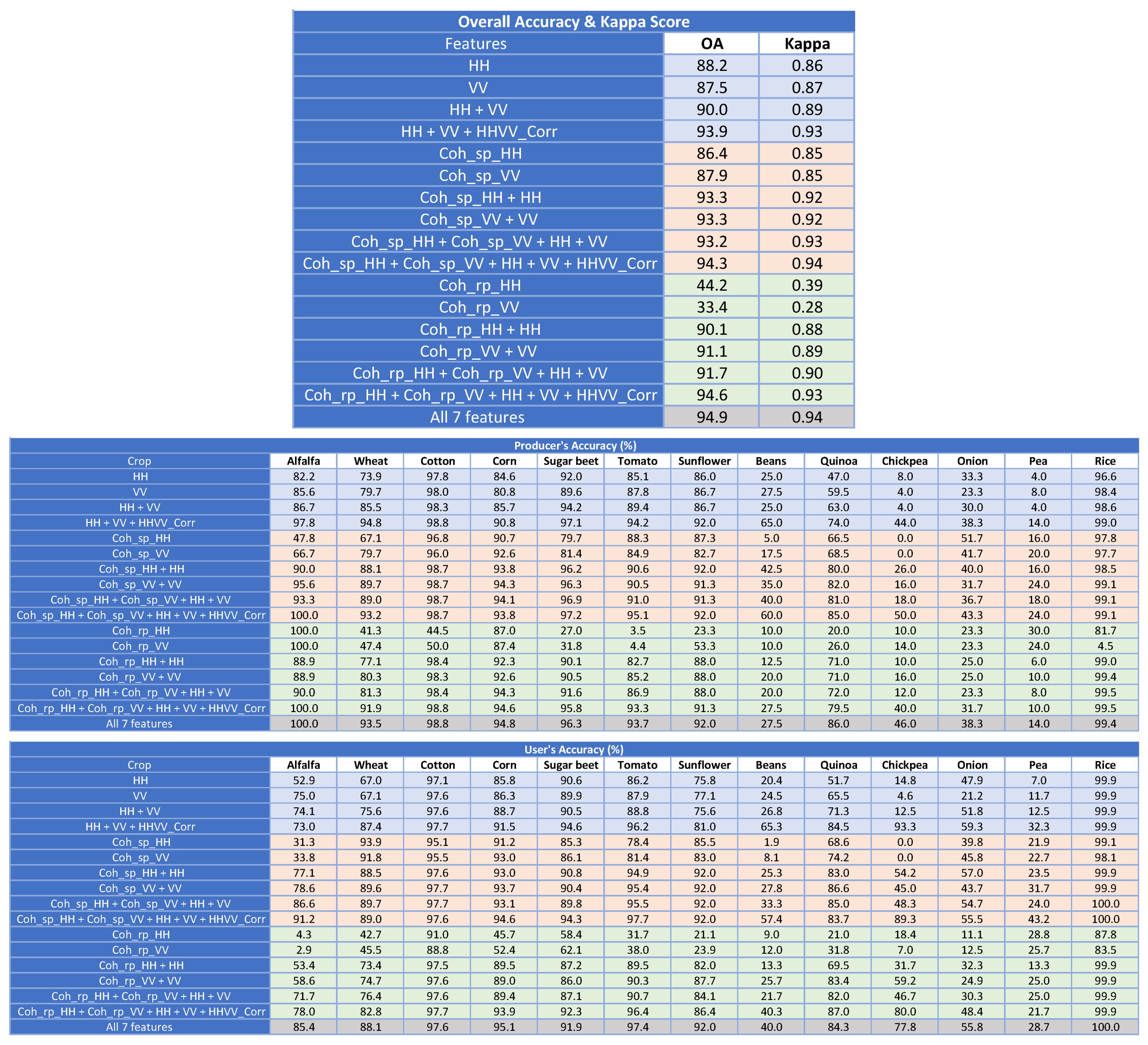
3.2.4. Results at Field Level with Pauli Channels

The scores of the evaluation at field level of the classification tests run with P1 and P2 channels are shown in

Table 7. Classification scores at field level with Pauli channels. Shading colour: blue for polarimetric features, pink for single-pass interferometric coherence features, green for repeat-pass interferometric coherence features, and grey for all features.

, and the OA values are also represented with a bar chart in Figure 9d. As in the case of HH and VV channels, the results exhibit an overall improvement with respect to the evaluation at pixel level, reaching OA values above 95% and Kappa equal to 0.95 for some feature sets in the Pauli basis.

The values of PA and UA for individual crops are also significantly improved in some cases with respect to HH and VV and with respect to the pixel-level evaluation. It is worth mentioning that chickpea, one of the crop type with low scores in all previous tests, reaches UA = 100% and PA = 62%, hence becoming much better classified, when the set of seven features is used. Moreover, in the best experiments with single-pass coherence (rows shaded in pink colour), the PA and UA values of the crop with worst results are not as extremely low as in other cases, since a sort of balance is achieved. For instance, with P1 + Coh_sp_P1 + P2 + Coh_sp_P2 + P1P2_Corr beans and chickpea exhibit UA and PA above 50%, and the values for onion and pea are also increased notably.

As a summary of the overall results, Figure 9 shows bar charts of the values of OA for all the sets of input features, from the HH and VV channels and the Pauli channels, and evaluated both at pixel and field level. The ordering and the colour coding employed for the bars is the same as in the previous tables. In these charts we can easily appreciate that the relative increment in OA provided by the interferometric coherence is larger when the evaluation is carried out at pixel level than when it is done at field level. In addition, it is evident that the highest improvements provided by coherence are reached when a single polarimetric channel is used.

4. Discussion

The classification results shown in this work can be compared with those obtained in previous experiments with time series of X-band SAR data, e.g., [14,18,19,20], but always taking into account that each study about crop classification has unique features, including the number and specificity of crop species present, and the SAR data available. This complicates comparison in absolute terms and has to be considered to draw right conclusions. For instance, the time span covered by the satellite images in this work is only 3 months and corresponds to summer, like in [19], whereas in other works there were images covering 5 to 7 months [14,18,20].

However, since the objective of this work is to assess the contribution of TanDEM-X interferometric products, it is important to quantify the added value of the sets of input features that include interferometric coherence with respect to those that do not consider them. To measure that added value, we defined as baseline cases the classification experiments based on polarimetric features, because they have demonstrated [19,20] to outperform the results based only on backscattering coefficient features [14]. For the particular dataset at hand, the OA obtained by the polarimetric features is 90–91% at pixel level and 93–95% at field level, depending on whether the linear channels (HH,VV) or the Pauli channels (P1,P2) are employed. These values are similar to the best results obtained in the literature with X-band data [19], despite they were obtained over different crop types and with different radar data. Moreover, results based on the exploitation of single polarimetric channels (HH or VV) are of interest because single-pol images exhibit better spatial resolution and double coverage with respect to the HHVV dual-pol mode. Therefore, single-pol results could offer a good crop mapping product wherever spatial resolution is important, e.g., in intensive farming areas with small parcels.

The overall classification score obtained by including the dual-pol single-pass coherence values as input features improves by 2% with respect to the dual-pol baseline case, reaching 92%. More notably, in single-pol mode the increase in OA is 10% for the HH channel and 8% for the VV channel, reaching 87% and 88%, respectively. The improvement is more significant over tall crops, like corn and quinoa in the studied site, because in these cases single-pass interferometry provides sensitivity to the vertical structure of the plants. The main drawback of single-pass interferometry for crop-type mapping is the requirement of a large baseline (spatial separation between the two satellites), which in TanDEM-X is normally much shorter than the one exploited in this experiment. As a result, for the moment this result is of limited applicability in other scenarios.

Regarding repeat-pass interferometry, the tests carried out at pixel level using consecutive TanDEM-X images, i.e., acquired with a separation of 11 days, provide OA values slightly below the ones provided by single-pass coherence (OA 1–3% lower). However, the repeat-pass coherence values at HH and VV channels are clearly complementary to the backscattering coefficient, since their addition improves the individual performances by 6–7%. Furthermore, in the tests evaluated at field level the dual-pol results provide the same score as with single-pass coherences (OA above 94%). Compared to a past study on the contribution of X-band repeat-pass coherence for crop-type mapping [18], in which it was unclear, here we have demonstrated its added value when compared to the backscattering coefficient in single-pol cases, and also providing classification scores very close to those achieved by using polarimetric features from dual-pol data. Contrarily to single-pass, repeat-pass interferometry can be applied with time series of images acquired by a single satellite, so it is not restricted to the TanDEM-X mission. Consequently, this technique may constitute a very good complement to all the efforts performed so far with time series of SAR images for crop classification.

5. Conclusions

The tests carried out in this work have demonstrated the suitability of interferometric data, acquired at X band by the TanDEM-X sensor, to classify crop types. Both single-pass coherence and repeat-pass coherence have shown their added value as input features for the classifier with respect to the backscattering coefficient and other polarimetric features.

In the case of single-pass interferometry, which has been tested for the first time in this work for crop classification, coherence contributes to improve the classification accuracy in both the dual-pol and the single-pol cases. This contribution, which is more notable over tall crops, requires that the interferometric baseline is large enough to guarantee sensitivity to short vegetation, as it was during the science phase of TanDEM-X in 2015.

Repeat-pass interferometry has been also tested in this work by combining consecutive TanDEM-X images. The overall classification scores are slightly below the ones provided by single-pass coherence, but repeat-pass coherence is clearly complementary to the backscattering coefficient at both HH and VV channels. In fact, when evaluated at field level, results are coincident for both single-pass and repeat-pass cases.

Finally, we have also observed that the representation of the dual-pol data in the Pauli basis improves slightly the performance of the classifier, producing the absolute best scores.

All these results are encouraging despite the present work is obviously partial (not all crop types are present) and, hence, can not be generalised to any dataset. In particular, the available satellite observation interval only lasted 3 months (June to August) and hence covered partially the calendar of some of the crops, for which indeed the classification performed worst. Therefore, a more complete experiment covering the whole calendar of the crops in the observed scene would be recommended to fully evaluate the contribution of the interferometric coherence, both single-pass and repeat-pass. In addition, attending to the observed seasonal variation of interferometric and polarimetric features, a future investigation on the impact of acquisition time on classification accuracy would be of interest, especially if conducted to optimise the acquisition schedule and to reduce the data requirements.

Regarding the use of other products, besides the coherence, derived from single-pass interferometry by TanDEM-X, the interferometric phase, once converted to DEM, could provide also a valuable information related to the plants type and height, so it could contribute to crop-type mapping. Examples of vegetation height estimates obtained over agricultural crops by TanDEM-X can be found in [50,51]. Therefore, future works should consider the application of TanDEM-X-derived vegetation height for crop-type mapping.

From the point of view of the sensor complexity, single-pass interferometry is the most demanding technique employed here, because it requires two synchronised satellites flying in close formation, whereas repeat-pass interferometry only needs a single satellite. In this sense, the use of repeat-pass coherence in single-pol data (i.e., only one polarimetric channel, HH or VV) improves the OA by 6–7% with respect to the individual backscattering coefficient, which constitutes a remarkable result and exhibits an important future potential because of the simple acquisition scheme that is required (time series of single-pol radar images) and the advantages of spatial resolution and coverage of single-pol images. In this context, the potential use of the cross-polarimetric channel (VH) and its associated coherence and backscatter, either alone or in conjunction with one co-polar channel, should be analysed in the future, since that channel is known to be dominated by the presence of volume scattering from vegetation and it usually outperforms other channels in crop-type mapping.

In the current Earth observation context, in which the Sentinel-1 constellation is providing wide-coverage C-band radar images every 6 days, the potential specific contribution of these X-band satellites, like TerraSAR-X, TanDEM-X and PAZ, would be their capability to classify crops with finer spatial resolution. This would help to solve, at least partially, the limitation found in recent crop-type mapping experiments with Sentinel-1 due to the small size of the fields [29,30].

References

1. Krieger, G.; Moreira, A.; Fiedler, H.; Hajnsek, I.; Werner, M.; Younis, M.; Zink, M. TanDEM-X: A satellite formation for high-resolution SAR interferometry. IEEE Trans. Geosci. Remote Sens. 2007, 45, 3317–3341. [Google Scholar] [CrossRef] [Green Version]
2. Rizzoli, P.; Martone, M.; Gonzalez, C.; Wecklich, C.; Borla Tridon, D.; Bräutigam, B.; Bachmann, M.; Schulze, D.; Fritz, T.; Huber, M.; et al. Generation and performance assessment of the global TanDEM-X digital elevation model. ISPRS J. Photogramm. Remote. Sens. 2017, 132, 119–139. [Google Scholar] [CrossRef] [Green Version]
3. Kugler, F.; Schulze, D.; Hajnsek, I.; Pretzsch, H.; Papathanassiou, K.P. TanDEM-X Pol-InSAR Performance for Forest Height Estimation. IEEE Trans. Geosci. Remote Sens. 2014, 52, 6404–6422. [Google Scholar] [CrossRef]
4. Abdullahi, S.; Kugler, F.; Pretzsch, H. Prediction of stem volume in complex temperate forest stands using TanDEM-X SAR data. Remote. Sens. Environ. 2016, 174, 197–211. [Google Scholar] [CrossRef]
5. Martone, M.; Rizzoli, P.; Wecklich, C.; Gonzalez, C.; Bueso-Bello, J.L.; Valdo, P.; Schulze, D.; Zink, M.; Krieger, G.; Moreira, A. The global forest/non-forest map from TanDEM-X interferometric SAR data. Remote. Sens. Environ. 2018, 205, 352–373. [Google Scholar] [CrossRef]
6. Rankl, M.; Braun, M. Glacier elevation and mass changes over the central Karakoram region estimated from TanDEM-X and SRTM/X-SAR digital elevation models. Ann. Glaciol. 2016, 57, 273–281. [Google Scholar] [CrossRef] [Green Version]
7. Poland, M.P. Time-averaged discharge rate of subaerial lava at Kilauea Volcano, Hawaii, measured from TanDEM-X interferometry: Implications for magma supply and storage during 2011–2013. J. Geophys. Res. Solid Earth 2014, 119, 5464–5481. [Google Scholar] [CrossRef]
8. McNairn, H.; Brisco, B. The application of C-band polarimetric SAR for agriculture: A review. Can. J. Remote Sens. 2004, 30, 525–542. [Google Scholar] [CrossRef]
9. Steele-Dunne, S.C.; McNairn, H.; Monsivais-Huertero, A.; Judge, J.; Liu, P.; Papathanassiou, K. Radar Remote Sensing of Agricultural Canopies: A Review. IEEE J. Sel. Top. Appl. Earth Obs. Remote Sens. 2017, 10, 2249–2273. [Google Scholar] [CrossRef] [Green Version]
10. Blaes, X.; Vanhalle, L.; Defourny, P. Efficiency of crop identification based on optical and SAR image time series. Remote. Sens. Environ. 2005, 96, 352–365. [Google Scholar] [CrossRef]
11. Skriver, H. Crop Classification by Multitemporal C-and L-Band Single-and Dual-Polarization and Fully Polarimetric SAR. IEEE Trans. Geosci. Remote. Sens. 2012, 50, 2138–2149. [Google Scholar] [CrossRef]
12. Bargiel, D. A new method for crop classification combining time series of radar images and crop phenology information. Remote. Sens. Environ. 2017, 198, 369–383. [Google Scholar] [CrossRef]
13. Foody, G.M.; Curran, P.J.; Groom, G.B.; Munro, D.C. Crop Classification With Multi-temporal X-band SAR Data. In Proceedings of the International Geoscience and Remote Sensing Symposium, ’Remote Sensing: Moving Toward the 21st Century’, Edinburgh, UK, 12–16 September 1988; Volume 1, pp. 217–220. [Google Scholar]
14. Bargiel, D.; Herrmann, S. Multi-temporal land-cover classification of agricultural areas in two European regions with high resolution spotlight TerraSAR-X data. Remote Sens. 2011, 3, 859–877. [Google Scholar] [CrossRef] [Green Version]
15. Sonobe, R.; Tani, H.; Wang, X.; Kobayashi, N.; Shimamura, H. Random forest classification of crop type using multi-temporal TerraSAR-X dual-polarimetric data. Remote Sens. Lett. 2014, 5, 157–164. [Google Scholar] [CrossRef] [Green Version]
16. Hütt, C.; Waldhoff, G. Multi-data approach for crop classification using multitemporal, dual-polarimetric TerraSAR-X data, and official geodata. Eur. J. Remote. Sens. 2018, 51, 62–74. [Google Scholar] [CrossRef]
17. Mirzaee, S.; Motagh, M.; Arefi, H.; Nooryazdan, M. Classification of agricultural fields using time series of dual polarimetry TerraSAR-X images. In International Archives of the Photogrammetry, Remote Sensing and Spatial Information Sciences; International Society of Photogrammetry and Remote Sensing (ISPRS): Heipke, Germany, 2014; Volume XL-2/W3, pp. 191–196. [Google Scholar] [CrossRef] [Green Version]
18. Sonobe, R.; Tani, H.; Wang, X.; Kobayashi, N.; Shimamura, H. Discrimination of crop types with TerraSAR-X-derived information. Phys. Chem. Earth Parts A/B/C 2015, 83–84, 2–13. [Google Scholar] [CrossRef] [Green Version]
19. Sonobe, R. Parcel-Based Crop Classification Using Multi-Temporal TerraSAR-X Dual Polarimetric Data. Remote Sens. 2019, 11, 1148. [Google Scholar] [CrossRef] [Green Version]
20. Busquier, M.; Lopez-Sanchez, J.M.; Bargiel, D. Added Value of Coherent Copolar Polarimetry at X-Band for Crop-Type Mapping. IEEE Geosci. Remote. Sens. Lett. 2020, 17, 819–823. [Google Scholar] [CrossRef]
21. Lee, J.S.; Papathanassiou, K.P.; Hajnsek, I.; Mette, T.; Grunes, M.R.; Ainsworth, T.; Ferro-Famil, L. Applying polarimetric SAR interferometric data for forest classification. In Proceedings of the IEEE International Geoscience and Remote Sensing Symposium, Seoul, Korea, 29 July 2005; Volume 7, pp. 4848–4851. [Google Scholar]
22. Ferro-Famil, L.; Kugler, F.; Pottier, E.; Lee, J.S. Forest Mapping and Classification at L band using POL-inSAR Optimal Coherence Set Statistics. In Proceedings of the EUSAR, Dresden, Germany, 16–18 May 2006. [Google Scholar]
23. Lee, J.S.; Pottier, E. Polarimetric Radar Imaging: From Basics to Applications; CRC Press: Boca Raton, FL, USA, 2009. [Google Scholar]
24. Li, X.; Pottier, E.; Guo, H.; Ferro-Famil, L. Urban land cover classification using polarimetric SAR interferometry. In Proceedings of the Sixth International Symposium on Digital Earth: Data Processing and Applications, Beijing, China, 9–12 September 2010; Society of Photo-Optical Instrumentation Engineers (SPIE) Conference Series: Bellingham, WA, USA; Volume 7841. [Google Scholar] [CrossRef]
25. Strozzi, T.; Dammert, P.B.G.; Wegmuller, U.; Martinez, J.; Askne, J.I.H.; Beaudoin, A.; Hallikainen, N.T. Landuse mapping with ERS SAR interferometry. IEEE Trans. Geosci. Remote Sens. 2000, 38, 766–775. [Google Scholar] [CrossRef]
26. Engdahl, M.E.; Hyyppa, J.M. Land-cover classification using multitemporal ERS-1/2 InSAR data. IEEE Trans. Geosci. Remote Sens. 2003, 41, 1620–1628. [Google Scholar] [CrossRef]
27. Sica, F.; Pulella, A.; Nannini, M.; Pinheiro, M.; Rizzoli, P. Repeat-pass SAR interferometry for land cover classification: A methodology using Sentinel-1 Short-Time-Series. Remote Sens. Environ. 2019, 232, 111277. [Google Scholar] [CrossRef]
28. Jacob, A.W.; Vicente-Guijalba, F.; Lopez-Martinez, C.; Lopez-Sanchez, J.M.; Litzinger, M.; Kristen, H.; Mestre-Quereda, A.; Ziółkowski, D.; Lavalle, M.; Notarnicola, C.; et al. Sentinel-1 InSAR Coherence for Land Cover Mapping: A Comparison of Multiple Feature-Based Classifiers. IEEE J. Sel. Top. Appl. Earth Observ. Remote Sens. 2020, 13, 535–552. [Google Scholar] [CrossRef] [Green Version]
29. Tomppo, E.; Antropov, O.; Praks, J. Cropland Classification Using Sentinel-1 Time Series: Methodological Performance and Prediction Uncertainty Assessment. Remote Sens. 2019, 11, 2480. [Google Scholar] [CrossRef] [Green Version]
30. Arias, M.; Campo-Bescós, M.A.; Álvarez Mozos, J. Crop Classification Based on Temporal Signatures of Sentinel-1 Observations over Navarre Province, Spain. Remote Sens. 2020, 12, 278. [Google Scholar] [CrossRef] [Green Version]
31. Morishita, Y.; Hanssen, R.F. Temporal Decorrelation in L-, C-, and X-band Satellite Radar Interferometry for Pasture on Drained Peat Soils. IEEE Trans. Geosci. Remote Sens. 2015, 53, 1096–1104. [Google Scholar] [CrossRef]
32. Parizzi, A.; Cong, X.Y.; Eineder, M. First Results from Multifrequency Interferometry. A Comparison of Different Decorrelation Time Constants at L, C and X Band. In Proceedings of the ESA FRINGE, Frascati, Italy, 30 November–4 December 2009. [Google Scholar]
33. Cloude, S.R. Polarisation: Applications in Remote Sensing; Oxford University Press: Oxford, UK, 2009. [Google Scholar]
34. Chen, H.; Cloude, S.R.; Goodenough, D.G. Forest Canopy Height Estimation Using TanDEM-X Coherence Data. IEEE J. Sel. Top. Appl. Earth Observ. Remote Sens. 2016, 9, 3177–3188. [Google Scholar] [CrossRef]
35. Lopez-Sanchez, J.M.; Vicente-Guijalba, F.; Erten, E.; Campos-Taberner, M.; Garcia-Haro, F.J. Retrieval of vegetation height in rice fields using polarimetric SAR interferometry with TanDEM-X data. Remote Sens. Environ. 2017, 192, 30–44. [Google Scholar] [CrossRef] [Green Version]
36. Zebker, H.A.; Villasenor, J. Decorrelation in interferometric radar echoes. IEEE Trans. Geosci. Remote Sens. 1992, 30, 950–959. [Google Scholar] [CrossRef] [Green Version]
37. Rosen, P.A.; Hensley, S.; Joughin, I.R.; Li, F.K.; Madsen, S.N.; Rodriguez, E.; Goldstein, R.M. Synthetic aperture radar interferometry. Proc. IEEE 2000, 88, 333–382. [Google Scholar] [CrossRef]
38. Gatelli, F.; Monti Guamieri, A.; Parizzi, F.; Pasquali, P.; Prati, C.; Rocca, F. The wavenumber shift in SAR interferometry. IEEE Trans. Geosci. Remote Sens. 1994, 32, 855–865. [Google Scholar] [CrossRef] [Green Version]
39. Martone, M.; Bräutigam, B.; Krieger, G. Quantization Effects in TanDEM-X Data. IEEE Trans. Geosci. Remote Sens. 2015, 53, 583–597. [Google Scholar] [CrossRef] [Green Version]
40. Breiman, L. Random Forests. Mach. Learn. 2001, 45, 5–32. [Google Scholar] [CrossRef] [Green Version]
41. Pedregosa, F.; Varoquaux, G.; Gramfort, A.; Michel, V.; Thirion, B.; Grisel, O.; Blondel, M.; Prettenhofer, P.; Weiss, R.; Dubourg, V.; et al. Scikit-learn: Machine Learning in Python. J. Mach. Learn. Res. 2011, 12, 2825–2830. [Google Scholar]
42. Available online: https://scikit-learn.org/ (accessed on 25 April 2020).
43. Stehman, S.V. Selecting and interpreting measures of thematic classification accuracy. Remote Sens. Environ. 1997, 62, 77–89. [Google Scholar] [CrossRef]
44. Lopez-Sanchez, J.M.; Cloude, S.R.; Ballester-Berman, J.D. Rice Phenology Monitoring by Means of SAR Polarimetry at X-Band. IEEE Trans. Geosci. Remote Sens. 2012, 50, 2695–2709. [Google Scholar] [CrossRef]
45. Martone, M.; Rizzoli, P.; Krieger, G. Volume Decorrelation Effects in TanDEM-X Interferometric SAR Data. IEEE Geosci. Remote Sens. Lett. 2016, 13, 1812–1816. [Google Scholar] [CrossRef]
46. Olesk, A.; Praks, J.; Antropov, O.; Zalite, K.; Arumäe, T.; Voormansik, K. Interferometric SAR Coherence Models for Characterization of Hemiboreal Forests Using TanDEM-X Data. Remote Sens. 2016, 8, 700. [Google Scholar] [CrossRef] [Green Version]
47. Schlund, M.; Magdon, P.; Eaton, B.; Aumann, C.; Erasmi, S. Canopy height estimation with TanDEM-X in temperate and boreal forests. Int. J. Appl. Earth Obs. Geoinf. 2019, 82, 101904. [Google Scholar] [CrossRef]
48. Lee, S.K.; Yoon, S.Y.; Won, J.S. Vegetation Height Estimate in Rice Fields Using Single Polarization TanDEM-X Science Phase Data. Remote Sens. 2018, 10, 1702. [Google Scholar] [CrossRef] [Green Version]
49. Touzi, R.; Lopes, A.; Bruniquel, J.; Vachon, P.W. Coherence estimation for SAR imagery. IEEE Trans. Geosci. Remote Sens. 1999, 37, 135–149. [Google Scholar] [CrossRef] [Green Version]
50. Rossi, C.; Erten, E. Paddy-Rice Monitoring Using TanDEM-X. IEEE Trans. Geosci. Remote Sens. 2015, 53, 900–910. [Google Scholar] [CrossRef] [Green Version]
51. Erten, E.; Lopez-Sanchez, J.M.; Yuzugullu, O.; Hajnsek, I. Retrieval of agricultural crop height from space: A comparison of SAR techniques. Remote Sens. Environ. 2016, 187, 130–144. [Google Scholar] [CrossRef] [Green Version]
Figure 1. Crop-type map with all fields available in the reference data.
Remotesensing 12 01774 g001
Figure 2. Crop calendar in 2015. The two red vertical lines denote the starting and final dates of the available TanDEM-X acquisitions.
Remotesensing 12 01774 g002
Figure 3. Images of some observables that are used for classification: (a) RGB polarimetric composite (Red = P1, Green = VV, Blue = P2) on 7 July 2015, (b) Single-pass coherence at HH channel on 7 July 2015, (c) Repeat-pass coherence at HH channel between 7 July 2015 and 18 July 2015.
Remotesensing 12 01774 g003
Figure 4. Temporal evolution of the backscattering coefficient at HH (blue) and VV (red) channels and their correlation (black) for all crop types. Dots represent the average values and the error bars denote the standard deviation of the estimates.
Remotesensing 12 01774 g004
Figure 5. Temporal evolution of the single-pass interferometric coherence at HH (blue) and VV (red) channels for all crop types. Dots represent the average values and the error bars denote the standard deviation of the estimates.
Remotesensing 12 01774 g005
Figure 6. Temporal evolution of the repeat-pass interferometric coherence at HH (blue) and VV (red) channels for all crop types. Dots represent the average values and the error bars denote the standard deviation of the estimates.
Remotesensing 12 01774 g006
Figure 7. Confusion matrix for the set of 7 features at HH and VV channels at pixel level.
Remotesensing 12 01774 g007
Figure 8. Maps with results of classification over the test areas. (a) Ground-truth data. (b) Crop-type map using only the polarimetric features: HH + VV + HHVV_Corr. (c) Crop-type map using the polarimetric features and the single-pass coherence: Coh_sp_HH + Coh_sp_VV + HH + VV + HHVV_Corr. (d) Crop-type map using the polarimetric features and the repeat-pass coherence: Coh_rp_HH + Coh_rp_VV + HH + VV + HHVV_Corr.
Remotesensing 12 01774 g008aRemotesensing 12 01774 g008b
Figure 9. Graphical representation of the OA values obtained by all sets of input features. Bar colour: blue for polarimetric features, pink for single-pass interferometric coherence features, green for repeat-pass interferometric coherence features, and grey for all features. (a) Pixel level. HH and VV channels. (b) Field level. HH and VV channels. (c) Pixel level. Pauli channels. (d) Field level. Pauli channels.
Remotesensing 12 01774 g009