Abstract
We analyzed the impacts of islands on suspended sediment concentration (SSC) in Zhoushan Coastal waters based on data from HY-1C, which was launched in September 2018 in China, carrying Coastal Zone Imager (CZI) and Chinese Ocean Color and Temperature Scanner (COCTS) on it for offshore observation. A new SSC retrieved model was established based on the relationship between in situ SSC and the reflectance in red and near infrared bands of CZI image. Fifteen CZI images obtained from October to December 2019 were applied to retrieve SSC in Zhoushan coastal waters. The results show that SSC in study area is 100–1600 mg·L−1. The SSC near islands changes obviously. Upstream of the islands, SSC is lower than downstream. During the flood and ebb, when the current passes through the islands, circumfluence will appear, under certain geophysical factors, generating Karman vortex streets downstream of the islands. The sediments were stirred by the fast speed current at the outer side of vortex street to the sea surface inducing higher SSC at the outer side of the vortex street, while the central sediments of the vortex street were lower. In the direction of ocean currents, the SSC of the vortex street downstream of islands is changing regularly, i.e., increasing, then decreasing and increasing again and then decreasing in a snaking vortex street whose length downstream is between 1000 and 8000 m long.
1. Introduction
Dynamic processes, such as the ocean waves, currents, tides and eddies, are complex and influential [1]. These dynamic environmental factors should be considered for offshore marine management. The interaction between the coastal seabed topography, islands and ocean currents is significant [2,3,4].
Eddies, as one important ocean dynamic factor, can induce the changes of many other ocean factors, such as the exchange of heat, nutrients and suspended matters [5]. Ocean eddies, mainly produced by baroclinic instability and density fronts, can induce ocean water upwelling and downwelling. Upwelling carries cold seawater and nutrients to the surface of the ocean, while the downwelling brings warm and nutrient-poor seawater back to the seabed [6,7]. As early as 1958, the British oceanographer Slobby applied acoustic technology to detect the presence of eddy in the ocean. Since an eddy is a marine water mass whose special features can be observed by satellite, many methods of eddy observation have been developed based on satellite technology [8,9]. In recent years, radar satellites can speculate the existence of eddy efficiently by detecting the velocity of sea surface currents [10]. Meanwhile, ocean color is another key factor in detecting the existence of eddies based on their impact on the concentration of suspended sediments, chlorophyll and organic matters as well as temperature in the ocean [11].
Waves and currents play an important role in transporting suspended matters in ocean, especially in coastal areas [12,13]. Remote sensing technology was first applied for the distribution of marine suspended matters observation in 1970 [14]. In the past 50 years, many researchers have devoted their studies to combining satellite data to analyze the changes in marine suspended matters [15,16,17] and the retrieving techniques of suspended sediment concentration have tended to be more mature [18,19,20]. Many water quality parameters, including suspended sediment concentrations [21], can be obtained from satellite remote sensing data [22,23]. Meanwhile, the Coastal Zone Imager (CZI) and Chinese Ocean Color and Temperature Scanner (COCTS), boarded on HY-1A and B, have greatly helped us in Chinese marine coastal zone management [24,25].
The Karman vortex street, a repeating pattern of swirling vortices, is caused by a process of vortex shedding, due to the unsteady separation of flow of fluids around obstacle bodies [26]. Being a special type of eddy, the Karman vortex street was first discovered by German scientist Theodore von Karman [27]. With the advent of later meteorological satellites, researchers began to pay attention to this interesting natural phenomenon in atmospheric [28,29]. Based on the analysis mentioned above, can the Karman vortex street be detected from the satellite by the change in suspended sediment concentration (SSC)?
In this paper, we analyzed the impacts of coastal islands on distribution of suspended sediment concentration based on satellite data obtained from a new launched satellite HY-1C, which has an advanced resolution in time and space.
2. Data and Method
2.1. Study Area
The Zhoushan Islands (121°30′~123°25′E, 29°32′~31°04’N) are located at the outside of Hangzhou Bay and south side of the Yangtze River estuary, in the East China Sea (Figure 1). The Zhoushan Islands area, including 1390 islands of different shapes and sizes, is China’s largest archipelago [30,31]. The territory is 182 km in length from east to west, 169 km in width from north to south, with the sea area of 20,800 km2 [31].
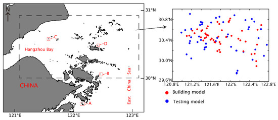
Figure 1.
Location of Hangzhou Bay and Zhoushan Islands (The black dotted box: the Zhoushan Islands; the small red boxes A, B, C, D; the places where the vortex streets appear).
The depth of the sea in the vortex streets area is mainly in the range of 7-16 m [32]. The northern part of Zhoushan coastal waters is close to the Yangtze River, the longest river in China [33]. The water flowing through the Qiantang River in Zhejiang Province flows into Hangzhou Bay from the west. Zhoushan coastal waters are in Hangzhou Bay, which is a strong tidal estuary and is dominated by the semidiurnal tide [34]. The direction and speed of the current in Hangzhou Bay is regularly changeable with time [35]. The bottom terrain of the Hangzhou Bay is undulating, and the tidal range increases from west to east, with the tidal peaks of the Qiantang River estuary, the water flowing southward of the Yangtze River estuary, and the East China Sea tide [36,37]. The mouth of Zhoushan coastal waters faces the East China Sea, and its SSC is significantly reduced [38]. In flood periods, low SSC seawater flows from the open sea into the Zhoushan [39].
Zhoushan sea area is characterized by a strong semidiurnal tidal current, which interacts with the islands, inducing the change in the direction and speed of the current [34]. This change is regular every day in Zhoushan coastal waters [40]. The Zhoushan Islands are located in the mouth Hangzhou Bay, whose average depth is around 9 m at a low tide and 13 m in flood periods. Hangzhou Bay includes shallow shoals in the northeast and a large sandbar in the south [41]. Runoff inflow of the Yangtze River and Qiantang River induces high SSC, low salinity and chloride ion concentration in Zhoushan coastal waters [32]. The smallest salinity value appears near the coast and it increases with the distance from the shore [42]. The climate of Zhoushan sea is dominated by the north subtropical monsoon. The sea surface temperature changes with the season, mainly affected by the local geographical and hydrological cycle, such as Kuroshio [43,44]. The detail information of study area and sampling points was show in Figure 1.
2.2. Satellite Data
Chinese HY-1C satellite, was launched in 2018. It was equipped with five payloads, including Chinese Ocean Color and Temperature Scanner (COCTS), Coastal Zone Imager (CZI), Ultraviolet Imagery (UV), Satellite Calibration Spectrometer (SCS), and Automatic Identification System (AIS). CZI can be applied not only for land observation, but also for effective ocean observation, especially for offshore, islands and coastal observations. CZI has red, green, blue and near infrared bands, with the spatial resolution of better than 50 m and the width of more than 950 km. In this study, fifteen CZI images from HY-C were applied to analyze suspended sediment distribution in Zhoushan Coastal waters. These images were obtained around 10:50 local time under clear sky conditions. The detailed information about the CZI images including the bands, resolution, applications of the CZI sensor is shown in the Table 1.

Table 1.
Details of HY-1C Coastal Zone Imager (CZI) sensor and date of data acquisition.
2.3. In Situ Data
Two field data collection campaigns were conducted from October to December 2019 (denoted by the small black square in Figure 1. One important survey was carried out to collect water samples from 100 stations at around 10:50 on 11 December 2019 using 15 fishing boats at different positions in the sampling area; their locations were changed and water samples were collected between 10:20 and 11:20, giving a total of 100 water samples used in this study. The SSC values of the water samples were measured in the laboratory: 50 were used to construct an SSC inverse model based on satellite data obtained synchronously, with the remaining 50 used to validate the model.
To study the changes in spectral characteristics induced by SSC and determine the wave bands sensitive to changes in SSC, the other survey was conducted on 27 October 2019, from 8:00 to 16:00. The remote-sensing reflectance (Rrs) and SSC were synchronously measured.
The Rrs value was detected using an ISI921VF visible, near-infrared (NIR) spectral radiometer with a spectral range of 380–1080 nm. The measured Rrs is calculated from Equation (1):
where is the radiance received by the ISI921VF above the sea–water surface; is the radiance of the sky; is the reflectance of the plate; is the radiance received by the ISI921VF above the plate; and ρ is the dimensionless air–water reflectance and is always in the range 0.022–0.050. ρ is calculated assuming a black ocean at wavelengths from 1000 to 1020 nm [45] and wavelength independence [46].
The depth of sampling area is mainly in the range of 4–20 m. Three samples were taken 1 m below the sea in every point using GCC2 plexiglass water bottle (3 L) and each sample was weighed, dried and measured, then averaged to get the sampled point value.
SSC, the per unit volume of particulate matter, was collected from underwater samples.
The depth of sampling area is mainly in the range of 4–20 m. Three samples were taken 1 m below the sea surface in every point using GCC2 plexiglass water bottle (3 L) and each sample was weighed, dried and measured, then averaged to get the sampled point value. Prior studies provided methods of suspended solid concentration measurements in river [47] and in sea water [48]. These water samples were first filtered, then dried for 24 hours at 40 ºC and reweighed for obtaining the SSC value [48]. Low salt content in Hangzhou Bay water, there is negligible effect on SSC measurement [47].
The tidal current of study area from March 10th to 11th, 2012 was measured by a direct reading ammeter SCL9-2 to qualitatively analyze the changing regularity of tidal current and flow direction. SCL9-2 can be used to measure the speed and direction of water at different depth in oceans, harbors, rivers, lakes, estuaries and it is especially suitable for shallow waters.
2.4. Satellite Data Processing
The primary products, including pixel brightness value of images in each band, called digital number, are needed when calculating the reflectance of atmospheric top from the digital number [49]. The process of calculating ground reflectance from the reflectance of the top of the atmosphere is called atmospheric correction [50].
Before the process of radiation calibration and atmospheric correction, we need to eliminate geometric distortion in satellite images—this step is called geometric correction. A polynomial geometric correction model was widely used in this step [51]. Generally, the positional accuracy was less than 0.5 pixels of the root mean square error (RMSE) in satellite images. Radiation calibration and atmospheric correction were performed on HY-1C data before SSC retrieving. Radiation calibration is the process of converting the digital number of the satellite images into a physical quantity such as radiance, reflectance or surface temperature [49]. This is done by reading the value of the gain and bias in the downloaded header file, and then calculating the reflectance with the formula of radiation calibration. The process of atmospheric correction mainly eliminates the influence of Rayleigh scattering and aerosol scattering [25]. The process was based on the 6SV radiative transfer mode [52], and calculating the Rayleigh scattering reflectance of atmospheric molecules by CZI Rayleigh lookup tables (LUT). The correction of aerosol scattering was based on the MODIS aerosol data [25]. The next step, after calculating the scattering reflectance of CZI, is to do the land mask based on the Normalized Difference Water Index (NDWX). Finally, we applied the atmospheric correction algorithm for HY-1C CZI in turbid waters to get the remote sensing reflectance which we can use in establishing the SSC model [53].
We collected the SSC data downstream of the island from the place of the vortex streets based on the SSC distribution images, plotting the obtained values to observe the changes in SSC along the vortex.
All calculations were performed in the software Python 3.7.
3. Result
3.1. Currents in Study Area
Dominated by semidiurnal tidal current in study area, the direction and speed of the current in study area change with time regularly (Figure 2). Taking a tidal cycle during 10–11 March 2012 as an example, the seawater in the East China Sea began to flow into the Zhoushan waters at 7:00 in the morning, flooding. Within two or three hours, the flow rate increased to the peak value, then the rising tide velocity began to decrease, and the flow direction continued to the west, but the westward angle became smaller and smaller. At 3 p.m., the flow began to move eastward, and the seawater flowed to the East China Sea. The eastward angle increased and the flow velocity decreased gradually. This continued until 10 p.m., and then the tide process began again. From 7 a.m. to 3 p.m. is the flood period, from 3 p.m. to 10 p.m. is the ebb, and then the flood is from 10 p.m. to 2 a.m. the next day. The ebb is from 2 a.m. to 7 a.m. The tide in study area presents the characteristics of irregular semidiurnal tide, there are two floods and ebbs in a day (Figure 2).
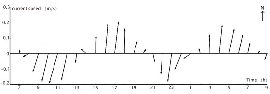
Figure 2.
Tidal velocity and direction during a tidal cycle during on10–11 March 2012 (The length of the arrow refers to the velocity of the currents and the direction measured counterclockwise from the east, the north is 90°).
The Zhoushan sea area is characterized by a strong semidiurnal tidal current and the tidal type is stable. Similar patterns and tidal features are repeated every day [40]. The tidal current, with its direction and speed changing with time regularly in a day, interacts with islands and induces different wake downstream of the islands.
3.2. A New SSC Estimation Model for HY-1C
The red and near-infrared bands are sensitive to suspended sediments in seawater [36,54]. A regression model was established based on the reflectance values averaged from of the nine-pixel values adjacent to the sampling point in the satellite data were collected, and with the in situ SSC values. The model is as follows:
where SSC is the suspended sediment concentration (mg·L−1), RRED and RNIR are respectively, the calibrated reflectance (The remote-sensing reflectance Rrs in units of 1/steradian.) in the third (red) and fourth (near-infrared red) bands after the atmospheric correction.
The other 50 different in situ SSC data were applied to evaluate the newly built model (Table 2 and Figure 3).
Table 2.
In situ data and model data of suspended sediment concentration (SSC).
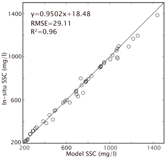
Figure 3.
Scatter plot for model SSC and in situ SSC verification.
Compared to the in situ SSC data, the result of the model-estimated result shows high consistency (RMSE is 29.11 mg·L−1, and the R-square is 0.96). Therefore, the new model is suitable for HY-1C to retrieve SSC in Zhoushan coastal waters. The information of scatter plot for model SSC and in situ SSC verification is shown in Figure 3.
3.3. Model-Retrieved SSC
3.3.1. SSC Distribution in Study Area
The samplings data were used to build the SSC inverse model and we applied this newly built model to retrieve the suspended sediment concentration from satellite images at different time. Using the new model, we obtained the distribution of SSC in study area from October to December 2019 (Figure 4). More than fifteen CZI images were obtained from the National Satellite Ocean Application Service (https://osdds.nsoas.org.cn) in China and six CZI images were taken as an example and analyzed in Figure 4. The SSC in study area is between 100 mg·L−1 and 1600 mg·L−1, showing high turbid water character. The SSC in the middle part of Hangzhou Bay, where the water depth is relatively shallow with the depth 5–9 m, is relatively higher, with SSC being in range of 1100–1500 mg·L−1. During the beginning and ending of ebb and flood periods, shown in Figure 4b,f, SSC is relatively lower in the study area, with the value being around 100–500 mg·L−1. Meanwhile, in the middle-flood and ebb periods, shown in Figure 4a,d,e, a higher SSC appears in the study area, with its value being around 900–1200 mg·L−1. The SSC distribution in the ebb period is obviously different from that in the flood period with high SSC area moving eastward in the ebb period. Meanwhile, the lower the current velocity is, the lower the SSC will be (Figure 4b,c,f). When the tidal current passes the islands in Zhoushan, in both ebb and flood, the tidal current will interact with islands, inducing the resuspension of the sediment near the islands. The sediment concentration downstream of the islands becomes higher.
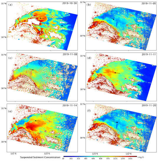
Figure 4.
The distribution of SSC retrieved from 6 CZI images (Figure 4 (a–f)) in the study area. (a–f) refers to satellite images of different date.
3.3.2. SSC around Islands
Dynamically, the islands will induce the Karman vortex street, whose outer speed is relatively fast, under a certain condition when the currents pass the islands. The depth of the sea in the vortex streets area is mainly in the range of 7-16 m [32]. The currents, because of the interaction with the islands, scour the bottom around islands, causing resuspension of suspended sediments. More than 45 Karman vortexes were founded and analyzed around the islands from HY-1C images, taking three vortex streets (the places are shown in Figure 1) as examples (Figure 5).
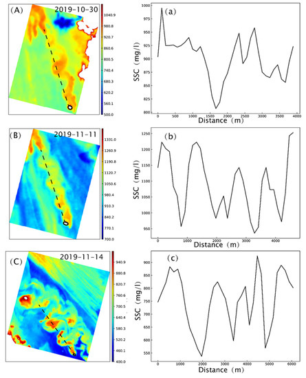
Figure 5.
The changes in SSC in the Karman vortex street observed in HY-1C CZI images ((A–C): The distribution of SSC in the vortex street; (a–c): the change in SSC sampled downstream of the vortex street; the dotted line in (A–C): sampling trajectory).
The external SSC is higher than that in center of the small vortex, and the SSC in the outside of the small vortex is higher than that of the surrounding waters. Therefore, we can clearly identify the vortex from the SSC images. They are more obvious in the study area at mid-flood period, and SSC changes as the length increases. Along the vortex street downstream from the islands, as shown in Figure 5a–c, the SSC increases first, then decreases, increases, and decreases, repeating until the vortex disappears. Generally, the length of the vortex streets in the study area is about 1000 to 8000 m.
4. Discussion
4.1. Applicability of New Model
HY-1C, a new Chinese satellite, is used for costal ocean environment observation [25]. Zhoushan is a coastal area with a high concentration of suspended sediments. The prior inversion models are not suitable for HY-1C to inverse SSC in this area [31]. The suspended sediment distribution obtained using the newly established model in Zhoushan coastal waters has a high consistency with in situ SSC as well as retrieved from other satellite data such as MODIS [19,55]. It is indicated that this new model is suitable for SSC retrieval in Zhoushan coastal waters.
4.2. The Factors Affecting Distribution of Suspended Sediment Concentration
Many natural factors, including fresh water injection, tidal currents, the bottom terrain, affect the distribution of SSC. The strong tide scouring the sediments at the bottom of the Hangzhou Bay and the sediments from the Changjiang River estuary flow into the bay with the tide are also important factors. These factors provide Hangzhou Bay with a strong tide and high concentration of suspended sediments [19,56]. Furthermore, when the current passes through the islands, it will wash the island and carry the sediment. The carried sediments move with the current and form a belt of hundreds of meters or kilometers behind the island.
4.3. Islands Induced Karman Vortex Streets Influenced SSC Distribution
The tidal current is affected by the islands during this movement. When passing through the island, the water flow is blocked and diverted to both the left and right sides of the island [57], forming vortex streets downstream of the island. The increased velocity around both sides of the island intensify the agitation of the water outside the vortex street and induce sediment resuspension. Meanwhile, in the center of the vortex, the convergency of water promotes the settlement of suspended sediments, resulting in low SSC there [58]. Therefore, the concentration of sediment outside the vortex is higher than in the center of the vortex [1,59].
5. Conclusions
Highlight findings of this paper include: (1) a new launched satellite HY-1C was applied for offshore observation; (2) a new SSC retrieved model was established based on CZI image from HY-1C; (3) the SSC near islands changes obviously, forming a snaking “SSC tape” with its length between 1000 and 8000 m downstream of the islands.
HY-1C, a Chinese new ocean satellite, has a great potential for offshore monitoring. The new SSC inverse model was built based on the relationship between the red and near-infrared band of CZI image and in situ SSC. The SSC retrieved from HY-1C CZI images using the new model shows a good consistency with in situ measurements. CZI images from HY-1C can be applied for offshore ocean color and dynamic environment monitoring.
The SSC in Zhoushan coastal waters is in the range of 100–1600 mg·L−1. The SSC in the study area is mainly influenced by tidal currents, underwater terrain and islands. The SSC downstream of the islands is higher than other areas, and there exists a “SSC tape” downstream of the islands.
The tidal current is affected by the islands (Figure 6). When passing the island, the water flow is blocked and diverted to both the left and right sides of the island, leading the current speed and direction to change downstream of the island. As the current passes through the islands, circumfluence will appear. Under certain geophysical factors, a vortex street with its length in the range of 1000 to 8000 m appears downstream of the islands. SSC changes as the length increases. The external SSC is higher than that in center of the small vortex, and the SSC in the outside of the vortex is higher than that of the surrounding waters. Therefore, we can clearly identify the vortex from the SSC images. They are more obvious in the study area at the mid-flood period.
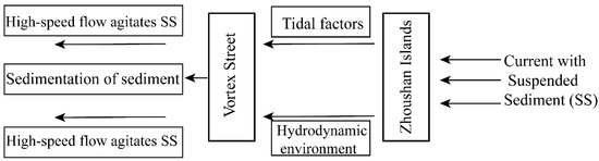
Figure 6.
Graphical abstract illustrates the impacts of Zhoushan Islands on suspended sediment distribution. When currents with suspended sediment pass through the Zhoushan Islands, forming the vortex street under the influence of tidal factors and hydrodynamic environment. The high-speed flow of the seawater agitates the suspended sediment to float outside the vortex while the central sediment is settled. Resulting the SSC increases, decreases, increases and repeating the change downstream the islands.
The mechanism of the impacts of the islands on SSC distribution lies in the islands affecting the hydrodynamic environment and inducing the formation of a Karman vortex street (Figure 6). The high-speed flow of the seawater outside the vortex agitates the SSC to float, inducing higher SSC outside the vortex street and lower SSC in the center. The SSC fluctuates in the vortex street of the islands, forming a snaking “SSC tape”, i.e., SSC increases, decreases, increases and reduces, repeating these changes until the vortex street disappears.
Author Contributions
L.C. and M.Z. jointly conducted the research, data collecting, processing, analysis, and manuscript writing. J.L. worked on the data collecting and advised the research project. D.T. designed and advised the research project and provided project support; J.Z. assisted paper editing. All authors have read and agreed to the published version of the manuscript.
Funding
This work is jointly supported by the following research projects: The Planning Program of Science and Technology of Zhoushan (2016C41018); Research Project of Zhejiang Department of Education (Y201840279); Guangdong Key Laboratory of Ocean Remote Sensing (South China Sea Institute of Oceanology Chinese Academy of Sciences) (2017B030301005-LORS2001, 2019BT2H594); The open Foundation from Marine Sciences in the First-Class Subjects of Zhejiang Province (11104060218); National Natural Science Foundation of China (41776183); National Key Project of Research and Development Plan of China “Research and Development of Ocean Big Data Analysis and Forecast Technology”, three-dimensional temperature and salinity prediction by big data analysis technology for marine dynamic environment (2016YFC1401904).
Acknowledgments
The data product of HY-1C satellite was provided by National Satellite Ocean Application Service, MNR of PRC.
Conflicts of Interest
The authors declare no conflict of interest.
References
- Aristegui, J.; Tett, P.; Hernández-Guerra, A.; Basterretxea, G.; Montero, M.F.; Wild, K.; Sangra, P.; Hernandez-Leon, S.; Canton-Garbin, M.; García-Braun, J.A.; et al. The influence of island-generated eddies on chlorophyll distribution: A study of mesoscale variation around Gran Canaria. Deep Sea Res. Part I Oceanogr. Res. Pap. 1997, 44, 71–96. [Google Scholar] [CrossRef]
- Davies, P.A.; Dakin, J.M.; Falconer, R.A. Eddy formation behind a coastal headland. J. Coast. Res. 1995, 11, 154–167. [Google Scholar]
- Chavanne, C.; Flament, P.; Lumpkin, R.; Dousset, B.; Bentamy, A. Scatterometer observations of wind variations induced by oceanic islands: Implications for wind-driven ocean circulation. Can. J. Remote Sens. 2002, 28, 466–474. [Google Scholar] [CrossRef]
- Roughan, M.; Terrill, E.J.; Largier, J.L.; Otero, M.P. Observations of divergence and upwelling around Point Loma, California. J. Geophys. Res. Ocean. 2005, 110, C04011. [Google Scholar] [CrossRef]
- Munk, W.; Armi, L.; Fischer, K.; Zachariasen, F. Spirals on the sea. Proc. R. Soc. A Math. 2000, 456, 1217–1280. [Google Scholar] [CrossRef]
- Williams, R.; Follows, M. Oceanography: Eddies make ocean deserts bloom. Nature 1998, 394, 228–229. [Google Scholar] [CrossRef]
- Williams, R.; Follows, M. Physical transport of nutrients and the maintenance of biological production. In Ocean Biogeochemistry: The Role of the Ocean Carbon Cycle in Global Change; Springer: Berlin/Heidelberg, Germany, 2003. [Google Scholar]
- Cardellach, E.; Treuhaft, R.N.; Chao, Y.; Lowe, S.T.; Young, L.E.; Zuffada, C. Coastal GPS Altimetry for Eddy Monitoring; EGS—AGU—EUG Joint Assembly: Nice, France, 2003. [Google Scholar]
- Garreau, P.; Dumas, F.; Louazel, S.; Stegner, A.; Vu, L.B. High-Resolution Observations and Tracking of a Dual-Core Anticyclonic Eddy in the Algerian Basin. J. Geophys. Res. Ocean 2018, 23, 9320–9339. [Google Scholar] [CrossRef]
- Kim, S.Y. Observations of submesoscale eddies using high-frequency radar-derived kinematic and dynamic quantities. Cont. Shelf Res. 2010, 30, 1639–1655. [Google Scholar] [CrossRef]
- Karoui, I.; Chauris, H.; Garreau, P.; Craneguy, P. Multi-resolution eddy detection from ocean color and Sea Surface Temperature images. In Proceedings of the OCEANS 2010 IEEE—Sydney, Sydney, Australia, 24–27 May 2010. [Google Scholar]
- Lopes, J.F.; Ferreira, J.A.; Cardoso, A.C.; Rocha, A.C. Variability of temperature and chlorophyll of the Iberian Peninsula near costal ecosystem during an upwelling event for the present climate and a future climate scenario. J. Mar. Syst. 2014, 129, 271–288. [Google Scholar] [CrossRef]
- Park, K.A.; Lee, M.S.; Park, J.E.; Ullman, D.; Cornillon, P.C.; Park, Y.J. Surface currents from hourly variations of suspended particulate matter from Geostationary Ocean Color Imager data. Int. J. Remote Sens. 2018, 39, 1929–1949. [Google Scholar] [CrossRef]
- Clarke, G.L.; Ewing, G.C.; Lorenzen, C.J. Spectra of Backscattered Light from the Sea Obtained from Aircraft as a Measure of Chlorophyll Concentration. Science 1970, 167, 1119–1121. [Google Scholar] [CrossRef] [PubMed]
- Spyrakos, E.; Vilas, L.; Torres, J.; Barton, E.D. Remote sensing chlorophyll a of optically complex waters: Application of a regionally specific chlorophyll-a algorithm for MERIS full resolution data during an upwelling cycle. Remote Sens. Environ. 2011, 115, 2471–2485. [Google Scholar] [CrossRef]
- Kopelevich, O.V.; Vazyulya, S.V.; Sheberstov, S.V. Suspended matter in the surface layer of the southeastern Baltic from satellite data. Oceanology 2016, 56, 46–54. [Google Scholar] [CrossRef]
- Burenkov, V.I.; Goldin, Y.A.; Kravchishina, M.D. The distribution of the suspended matter concentration in the Kara Sea in September 2007 based on ship and satellite data. Oceanology 2010, 50, 798–805. [Google Scholar] [CrossRef]
- Eurico, D.; Ko, D. Short-term Influences on Suspended Particulate Matter Distribution in the Northern Gulf of Mexico: Satellite and Model Observations. Sensors 2008, 8, 4249–4264. [Google Scholar] [CrossRef]
- Wang, F.; Zhou, B.; Xu, J.; Song, L.; Wang, X. Application of neural network and MODIS 250m imagery for estimating suspended sediments concentration in Hangzhou Bay, China. Environ. Geol. 2009, 56, 1093–1101. [Google Scholar] [CrossRef]
- Yang, X.; Sokoletsky, L.; Wei, X.; Fang, S. Suspended sediment concentration mapping based on the MODIS satellite imagery in the East China inland, estuarine, and coastal waters. Chin. J. Oceanol. Limnol. 2017, 35, 39–60. [Google Scholar] [CrossRef]
- Mobley, C.D. Radiative transfer in the ocean ☆. In Encyclopedia of Ocean Sciences; Elsevier: Bellevue, DC, USA, 2013; pp. 619–628. [Google Scholar]
- Volpe, V.; Silvestri, S.; Marani, M. Remote sensing retrieval of suspended sediment concentration in shallow waters. Remote Sens. Environ. 2011, 115, 44–54. [Google Scholar] [CrossRef]
- Kiyomoto, Y.; Iseki, K.; Okamura, K. Ocean Color Satellite Imagery and Shipboard Measurements of Chlorophyll a and Suspended Particulate Matter Distribution in the East China Sea. J. Oceanogr. 2001, 57, 37–45. [Google Scholar] [CrossRef]
- Li, S.J.; Mao, T.M.; Pan, D.L. A study quality and availability of COCTS images of HY-1 satellite by simulation. Acta Oceanol. Sin. 2002, 4, 495–540. [Google Scholar]
- Chen, X.; Zhang, J.; Tong, C.; Liu, R.; Mu, B.; Ding, J. Retrieval Algorithm of Chlorophyll-a Concentration in Turbid Waters from Satellite HY-1C Coastal Zone Imager Data. J. Coast. Res. 2019, 90, 146. [Google Scholar] [CrossRef]
- Thompson, M.C.; Radi, A.; Rao, A.; Sheridan, J.; Hourigan, K. Low-Reynolds-number wakes of elliptical cylinders: From the circular cylinder to the normal flat plate. J. Fluid Mech. 2014, 751, 570–600. [Google Scholar] [CrossRef]
- Karman, T.V. On the statistical theory of turbulence. Proc. Natl. Acad. Sci. USA 1937, 23, 98–105. [Google Scholar] [CrossRef] [PubMed]
- Chopra, K.P.; Hubert, L.F. Karman Vortex-Streets in Earth’s Atmosphere. Nature 1964, 203, 1341–1343. [Google Scholar] [CrossRef]
- Chopra, K.P.; Hubert, L.F. Karman vortex streets in wakes of islands. AIAA J. 1965, 3, 1941–1943. [Google Scholar] [CrossRef]
- Zhang, S.Y.; Wang, L.; Wang, W.D. Algal communities at Gouqi island in the Zhoushan archipelago, China. J. Appl. Phycol. 2008, 20, 853–861. [Google Scholar] [CrossRef]
- Zhu, W.; Liu, X.; Hu, X.; Zhou, S.; Zhang, Y. Investigation on the iodine nutritional status and the prevalence of thyroid carcinoma in Zhoushan archipelago residents. J. Hyg. Res. 2012, 41, 79–82. [Google Scholar]
- Cai, L.N.; Tang, L.D.; Li, X.F.; Zheng, H.; Shao, W. Remote Sensing of Spatial-Temporal Distribution of Suspended Sediment and Analysis of Related Environmental Factors in Hangzhou Bay, China. Remote Sens. Lett. 2015, 6, 597–603. [Google Scholar] [CrossRef]
- Chen, S.L.; Zhang, G.A.; Yang, S.L.; Shi, J.Z. Temporal variations of fine suspended sediment concentration in the Changjiang River estuary and adjacent coastal waters, China. J. Hydrol. 2006, 331, 137–145. [Google Scholar] [CrossRef]
- Walker, H.J. Geomorphological development and sedimentation in Qiantang estuary and Hangzhou Bay. J. Coast. Res. 1990, 6, 559–572. [Google Scholar]
- Zhang, F.; Dai, C.; Xu, X.; Wang, C.; Ye, Q. Resource assessment of tidal current energy in Hangzhou Bay based on long term measurement. IOP Conf. Ser. Earth Envion. Sci. 2017, 68, 012017. [Google Scholar] [CrossRef]
- Pope, R.; Fry, E. Absorption spectrum (380–700 nm) of pure water.2. Integrating cavity measurements. Appl. Opt. 1997, 36, 8710–8723. [Google Scholar] [CrossRef] [PubMed]
- Gao, S.; Yu, G.; Wang, Y. Distributional features and fluxes of dissolved nitrogen, phosphorus and silicon in the Hangzhou Bay. Mar. Chem. 1993, 43, 65–81. [Google Scholar]
- Liu, J.; Liu, J.; He, X.; Chen, T.; Zhu, F.; Wang, Y.; Hao, Z.; Chen, P. Retrieval of total suspended particulate matter in highly turbid Hangzhou Bay waters based on geostationary ocean color imager. In Proceedings of the Remote Sensing of the Ocean, Sea Ice, Coastal Waters, and Large Water Regions 2017, SPIE, Bellinham, DC, USA, 13 October 2017. [Google Scholar]
- Zhu, Y.T.; Biao, Z.J.; Yong, S.W. The characteristics of tidal current distribution in Zhapu section of the Hangzhou Bay. Donghai Mar. Sci. 2002. [Google Scholar]
- Cao, Y.; Lin, B. Tidal characteristics of Hangzhou Bay. Zhejiang Wat. Cons Hydr. Coll. 2000, 12, 14–16. [Google Scholar]
- Liu, S.; Liu, Y.; Yang, G.; Qiao, S.; Li, C.; Zhu, Z.; Shi, X. Distribution of Major and Trace Elements in Surface Sediments of Hangzhou Bay in China. Acta Oceanol. Sin. 2012, 31, 89–100. [Google Scholar] [CrossRef]
- Fu, J.; Chen, C.; Chu, Y. Spatial–temporal variations of oceanographic parameters in the Zhoushan sea area of the East China Sea based on remote sensing datasets. Reg. Stud. Mar. Sci. 2019, 28. [Google Scholar] [CrossRef]
- Venkata, S.M.; Zhang, Q.; Pushpanjali, B. Sea Surface Temperature Climatology over Zhoushan Sea. Am. J. Earth Sci. 2016, 3, 1–5. [Google Scholar]
- Huang, Q.; Wu, J.; Jiang, Y.; Li, J. Variability of terrigenous dissolved organic matter as a response to coastal plume in Zhoushan area of the East China Sea. Acta Oceanol. Sin. 2011, 33, 66–73. [Google Scholar]
- Hale, G.M.; Querry, M.R. Optical Constant of Water in the 200-Nm to 200-Mm Wavelength Region. Appl. Opt. 1973, 12, 555–563. [Google Scholar] [CrossRef]
- Doxaran, D.; Froidefond, J.M.; Lavender, S.J.; Castaing, P. Spectral Signature of Highly Turbid Water Application with SPOT Data to Quantify Suspended Particulate Matter Concentration. Remote Sens. Environ. 2002, 81, 149–161. [Google Scholar]
- Dramais, G.; Camenen, B.; Coz, J.; Thollet, F.; Bescond, C.; Lagouy, M.; Buffet, A.; Lacroix, F. Comparison of standardized methods for suspended solid concentration measurements in river samples. In Proceedings of the E3S Web of Conferences, Berlin, Germany, 21–24 September 2018. [Google Scholar]
- Qiu, Z.F. A Simple Optical Model to Estimate Suspended Particulate Matter in Yellow River Estuary. Opt. Express 2013, 21, 27891–27904. [Google Scholar] [PubMed]
- Vermote, E.F.; El Saleous, N.; Justice, C.O.; Kaufman, Y.J.; Privette, J.L.; Remer, L. Atmospheric correction of visible to middle-infrared EOS-MODIS data over land surfaces: Background, operational algorithm and validation. J. Geophys. Res. 1997, 102, 17131. [Google Scholar] [CrossRef]
- Harriet, H.; Natsuyama, S.U.; Alan, P.W. Atmospheric Correction. Terr. Radiat. Transf. 1998. [Google Scholar] [CrossRef]
- Hadjimitsis, D.G.; Hadjimitsis, M.G.; Clayton, C.; Clarke, B.A. Determination of Turbidity in Kourris Dam in Cyprus Utilizing Landsat TM Remotely Sensed Data. Water Resour. Manag. 2006, 20, 449–465. [Google Scholar] [CrossRef]
- Lenoble, J.; Herman, M. Radiative transfer in the Earth’s atmosphere. Aerosol Remote Sens. 2013, 53–86. [Google Scholar]
- Tong, C.; Mu, B.; Liu, R.; Ding, J.; Zhang, M.; Xiao, Y.; Liang, X.; Chen, X. Atmospheric Correction Algorithm for HY-1C CZI over Turbid Waters. J. Coast. Res. 2019, 90, 156–163. [Google Scholar]
- Hou, P.; Wang, L.; Cao, G.; Yang, F. Analysis and research of remote sensing for suspended sediment in water. Proc. SPIE Int. Soc. Opt. Eng. 2004, 5239, 89–97. [Google Scholar] [CrossRef]
- Liu, W.; Yu, Z.; Zhou, B.; Jiang, J.; Ling, Z. Assessment of suspended sediment concentration at the Hangzhou Bay using HJ CCD imagery. J. Remote Sens. 2013, 17, 905–918. [Google Scholar]
- Su, J.; Wang, K. Changjiang River plume and suspended sediment transport in Hangzhou Bay. Cont. Shelf Res. 1989, 9, 93–111. [Google Scholar]
- Xie, D.; Wang, Z.; Gao, S.; Vriend, H.J.D. Modeling the tidal channel morphodynamics in a macro-tidal embayment, Hangzhou Bay, China. Cont. Shelf Res. 2009, 29, 1757–1767. [Google Scholar]
- Chung, Y.S.; Kim, H.S. Mountain-generated vortex streets over the Korea south sea. Int. J. Remote Sens. 2008, 29, 867–877. [Google Scholar]
- Davies, A.G.; Thorne, P.D. Modeling and measurement of sediment transport by waves in the vortex ripple regime. J. Geophys. Res. Ocean. 2005, 110. [Google Scholar] [CrossRef]
© 2020 by the authors. Licensee MDPI, Basel, Switzerland. This article is an open access article distributed under the terms and conditions of the Creative Commons Attribution (CC BY) license (http://creativecommons.org/licenses/by/4.0/).