Fast Split Bregman Based Deconvolution Algorithm for Airborne Radar Imaging


 ,
, 
Abstract

1. Introduction
2. Problem Formulation
2.1. Signal Model
2.2. Regularization Problem
3. Solution of the Optimization Problem
3.1. Solution with SBA
3.2. Solution with the Proposed FSBA
3.3. Regularization Parameter
4. Experiments
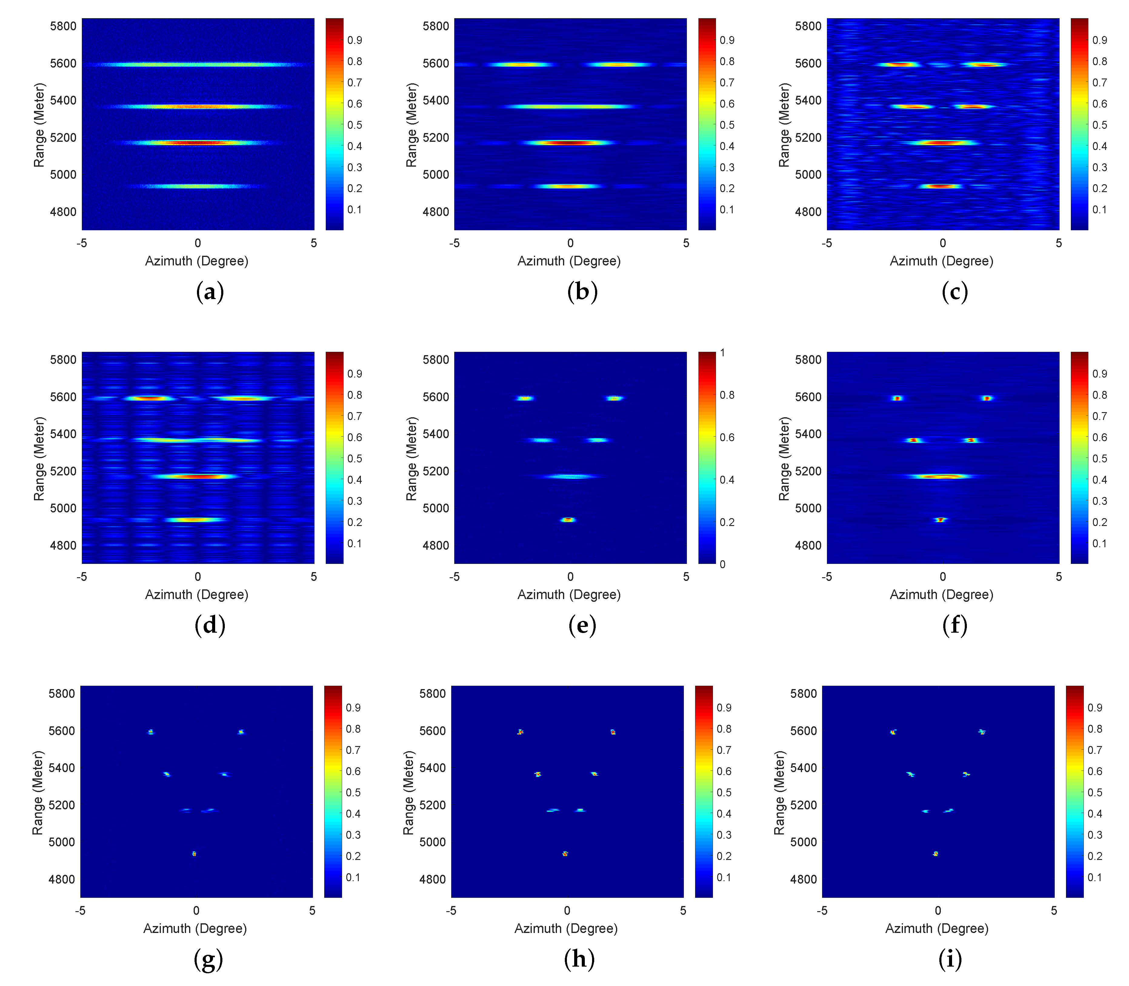
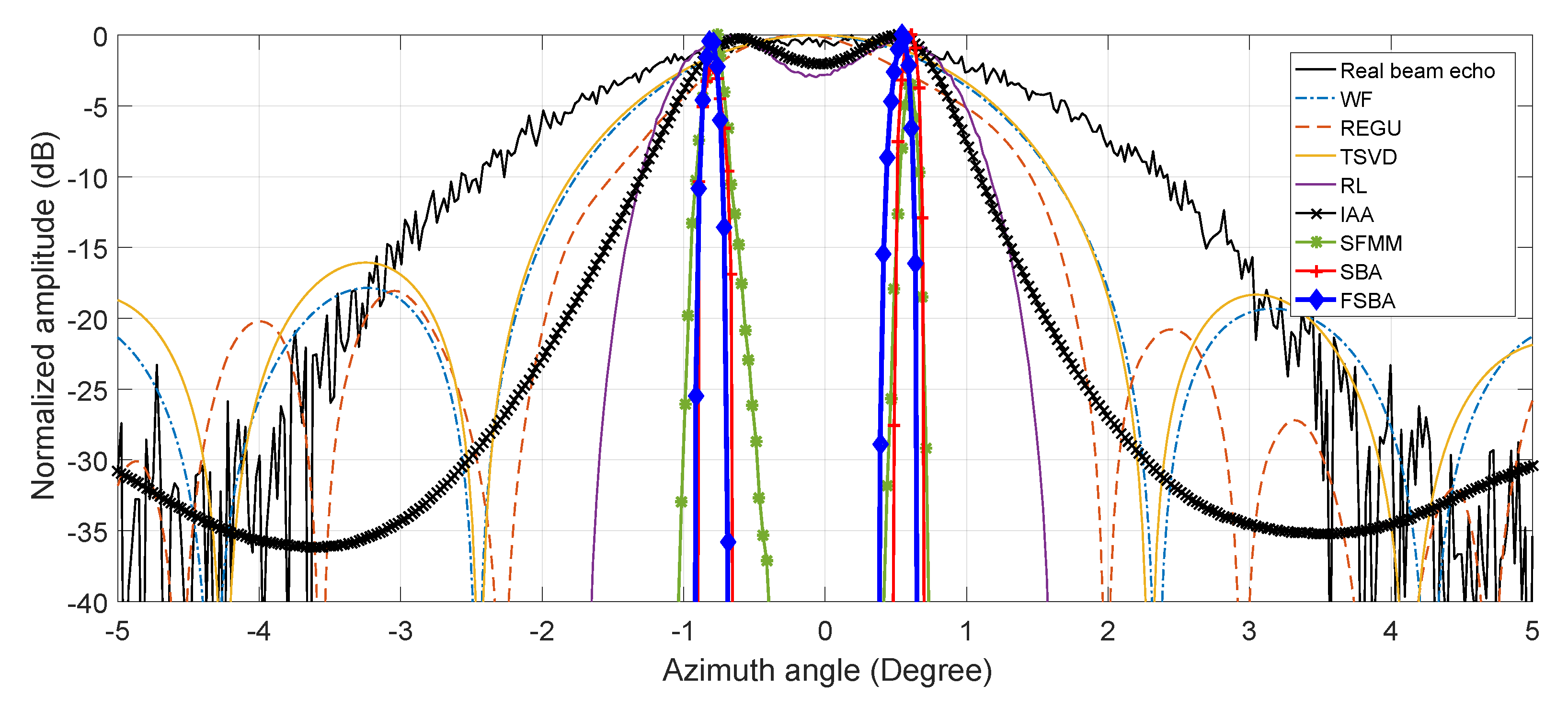
4.1. Simulation
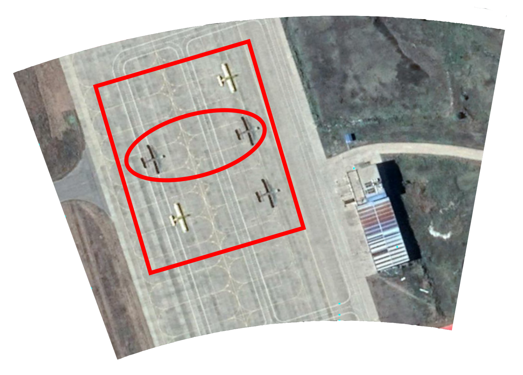
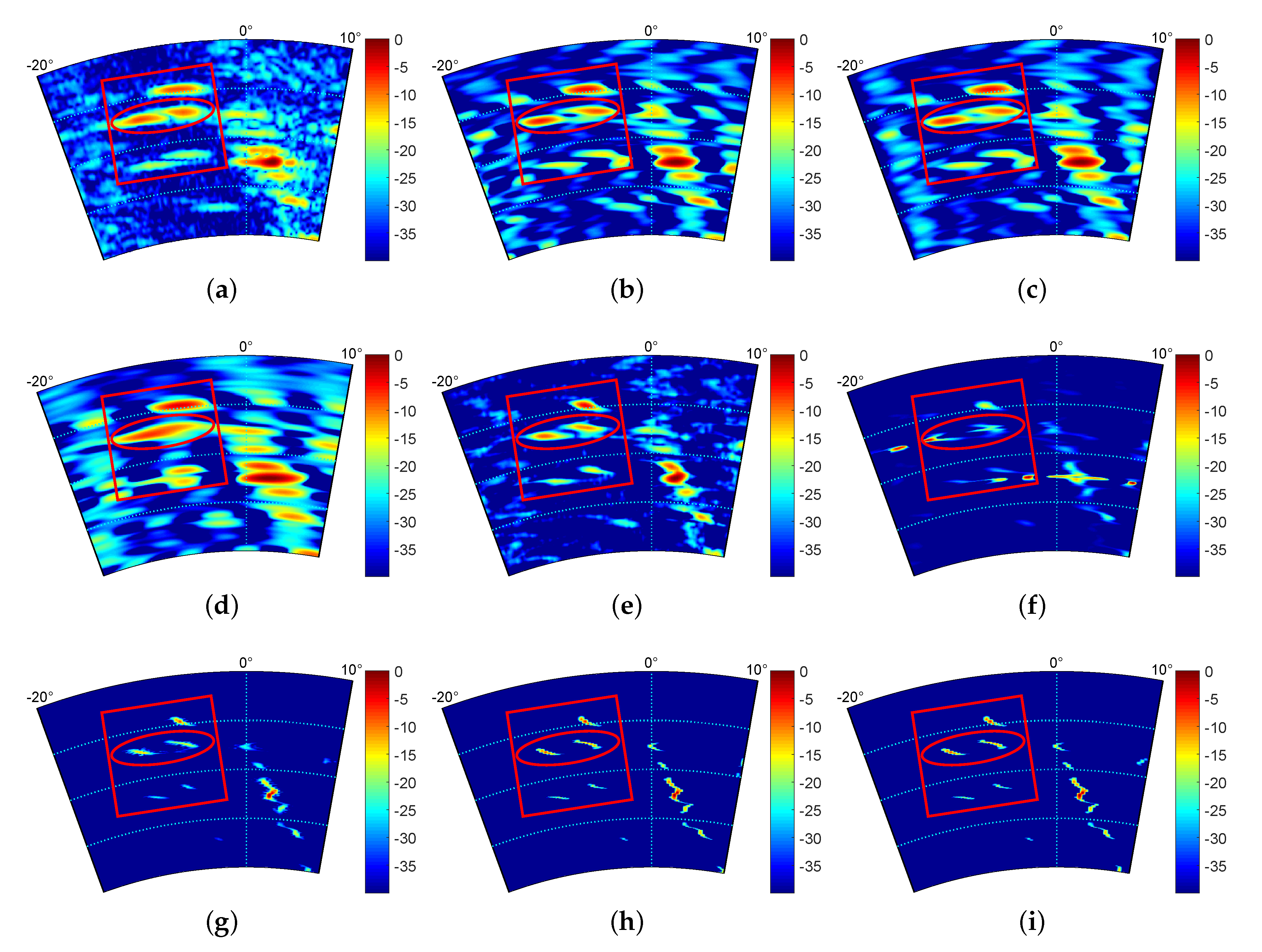
4.2. Real Data Processing
4.3. Assessment of Computing Time
5. Conclusions
Author Contributions
Funding
Conflicts of Interest
References
- Uttam, S.; Goodman, N.A. Superresolution of coherent sources in real-beam data. IEEE Trans. Aerosp. Electron. Syst. 2010, 46, 1557–1566. [Google Scholar] [CrossRef]
- Zhang, Y.; Mao, D.; Zhang, Q. Airborne forward-looking radar superresolution imaging using iterative adaptive approach. IEEE J. Sel. Top. Appl. Earth Obs. Remote. Sens. 2019, 12, 2044–2054. [Google Scholar] [CrossRef]
- Li, Z.; Li, S.; Liu, Z. Bistatic Forward-Looking SAR MP-DPCA Method for Space–Time Extension Clutter Suppression. IEEE Trans. Geosci. Remote. Sens. 2020. [Google Scholar] [CrossRef]
- Dropkin, H.; Ly, C. Superresolution for scanning antenna. In Proceedings of the 1997 IEEE National Radar Conference, Ann Arbor, MI, USA, 13 May 1997; pp. 306–308. [Google Scholar]
- Liu, G.; Yang, K.; Sykora, B. Range and azimuth resolution enhancement for 94 GHz real-beam radar. In Proceedings of the XII International Society for Optics and Photonics, Radar, Sensor Technology, Orlando, FL, USA, 15 April 2008; SPIE: Bellingham, WA, USA, 2008; Volume 6947, pp. 1–6. [Google Scholar]
- Zhang, Y.; Jakobsson, A.; Yin, Z.; Huang, Y.; Yang, J. Wideband sparse reconstruction for scanning radar. IEEE Trans. Geosci. Remote. Sens. 2018, 99, 1–14. [Google Scholar] [CrossRef]
- Cruz, C.; Mehta, R.; Katkovnik, V. Single image super-resolution based on Wiener filter in similarity domain. IEEE Trans. Image Process. 2017, 27, 1376–1389. [Google Scholar] [CrossRef]
- Doğu, S.; Akıncı, M.N.; Çayören, M.; Akduman, I. Truncated singular value decomposition for through-the-wall microwave imaging application. IET Microwaves Antennas Propag. 2019, 14, 260–267. [Google Scholar] [CrossRef]
- Kang, M.S.; Kim, K.T. Compressive sensing based SAR imaging and autofocus using improved Tikhonov regularization. IEEE Sensors J. 2019, 19, 5529–5540. [Google Scholar] [CrossRef]
- Campbell, J.F.; Lin, B.; Nehrir, A.R. Super-resolution technique for CW lidar using Fourier transform reordering and Richardson–Lucy deconvolution. Opt. Lett. 2014, 39, 6981–6984. [Google Scholar] [CrossRef]
- Raju, C.; Reddy, T.S. MST radar signal processing using iterative adaptive approach. Geosci. Lett. 2018, 5, 1–10. [Google Scholar]
- Zheng, Y.; Wu, F.; Shim, H.J. Sparse Unmixing for Hyperspectral Image with Nonlocal Low-Rank Prior. Remote Sens. 2019, 11, 2897. [Google Scholar]
- Ghasrodashti, E.; Karami, A.; Heylen, R. Spatial resolution enhancement of hyperspectral images using spectral unmixing and bayesian sparse representation. Remote Sens. 2017, 9, 541. [Google Scholar] [CrossRef]
- Zhang, Y.; Zhang, Q.; Li, C. Sea-Surface Target Angular Superresolution in Forward-Looking Radar Imaging Based on Maximum A Posteriori Algorithm. IEEE J. Sel. Top. Appl. Earth Obs. Remote. Sens. 2019, 12, 2822–2834. [Google Scholar] [CrossRef]
- Candes, E.J.; Wakin, M.B.; Boyd, S.P. Enhancing sparsity by reweighted L1 minimization. J. Fourier Anal. Appl. 2007, 14, 877–905. [Google Scholar] [CrossRef]
- Zhang, Q.; Zhang, Y.; Huang, Y.; Zhang, Y. Azimuth superresolution of forward-looking radar imaging which relies on linearized bregman. IEEE J. Sel. Top. Appl. Earth Obs. Remote. Sens. 2019, 12, 2032–2043. [Google Scholar]
- Osher, S.; Goldstein, T. The split bregman method for L1 regularized problems. SIAM J. Imaging Sci. 2009, 2, 323–343. [Google Scholar]
- Cai, J.F.; Osher, S.; Shen, Z. Split bregman methods and frame based image restoration. Siam J. Multiscale Model. Simul. 2009, 8, 337–369. [Google Scholar] [CrossRef]
- Zhang, Q.; Zhang, Y.; Mao, D. A bayesian superresolution method for forward-looking scanning radar imaging based on split bregman. In Proceedings of the IGARSS 2018-2018 IEEE International Geoscience and Remote Sensing Symposium, Valencia, Spain, 27 July 2018; pp. 5135–5138. [Google Scholar]
- Jazayeri, S.; Kazemi, N.; Kruse, S. Sparse blind deconvolution of ground penetrating radar data. IEEE Trans. Geosci. Remote. Sens. 2019, 57, 3703–3712. [Google Scholar] [CrossRef]
- Smith, D.S.; Gore, J.C.; Yankeelov, T.E.; Welch, E.B. Real-time compressive sensing MRI reconstruction using GPU computing and split bregman methods. Int. J. Biomed. Imaging 2012, 2012, 864827. [Google Scholar]
- Plonka, G.; Ma, J. Curvelet-wavelet regularized split Bregman iteration for compressed sensing. Int. J. Wavelets Multiresolution Inf. Process. 2011, 9, 79–110. [Google Scholar] [CrossRef]
- Ramani, S.; Fessler, J.A. A splitting-based iterative algorithm for accelerated statistical X-ray CT reconstruction. IEEE Trans. Med Imaging 2011, 31, 677–688. [Google Scholar] [CrossRef]
- Chen, D.; Zhu, S.; Cao, X. X-ray luminescence computed tomography imaging based on X-ray distribution model and adaptively split Bregman method. Biomed. Opt. Express. 2015, 6, 2649–2663. [Google Scholar] [CrossRef] [PubMed]
- Aggarwal, P.; Gupta, A. Accelerated fMRI reconstruction using matrix completion with sparse recovery via split bregman. Neurocomputing 2016, 216, 319–330. [Google Scholar] [CrossRef]
- Beck, A.; Teboulle, M. A fast iterative shrinkage thresholding algorithm for linear inverse problems. Siam J. Imaging Sci. 2009, 2, 183–202. [Google Scholar]
- Zhang, Q.; Zhang, Y.; Huang, Y. Sparse with Fast MM Superresolution Algorithm for Radar Forward-Looking Imaging. IEEE Access 2019, 7, 105247–105257. [Google Scholar]
- Osher, S.; Mao, Y.; Dong, B.; Yin, W. Fast linearized Bregman iteration for compressive sensing and sparse denoising. arXiv 2011, arXiv:1104.0262. [Google Scholar]
- Freund, R.W.; Zha, H. A look-ahead algorithm for the solution of general hankel systems. Numer. Math. 1993, 64, 295–321. [Google Scholar] [CrossRef]
- Zhang, Y.; Yin, Z.; Li, W.; Huang, Y.; Yang, J. Superresolution surface mapping for scanning radar: Inverse filtering based on the fast iterative adaptive approach. IEEE Trans. Geosci. Remote. Sens. 2018, 99, 1–18. [Google Scholar] [CrossRef]
- Glentis, G.O.; Jakobsson, A. Time-recursive IAA spectral estimation. IEEE Signal Process. Lett. 2010, 18, 111–114. [Google Scholar] [CrossRef]
- Kailath, T. Some new algorithms for recursive estimation in constant linear systems. Inf. Theory IEEE Trans. 1974, 19, 750–760. [Google Scholar]
- Bitmead, R.R.; Anderson, B.D.O. Asymptotically fast solution of toeplitz and related systems of linear equations. Linear Algebra Appl. 1980, 34, 103–116. [Google Scholar] [CrossRef]
- Glentis, G.O.; Jakobsson, A. Efficient implementation of iterative adaptive approach spectral estimation techniques. IEEE Trans. Signal Process. 2011, 59, 4154–4167. [Google Scholar] [CrossRef]
- Karlsson, J.; Rowe, W.; Xu, L.; Glentis, G.O.; Jian, L. Fast missing-data IAA with application to notched spectrum SAR. IEEE Trans. Aerosp. Electron. Syst. 2014, 50, 959–971. [Google Scholar] [CrossRef]
- Sidky, E.; Pan, X. Image reconstruction in circular cone-beam computed tomography by constrained, total variation minimization. Phys. Med. Biol. 2008, 53, 4777. [Google Scholar] [PubMed]
- Guangcan, L.; Zhouchen, L.; Shuicheng, Y.; Ju, S.; Yong, Y.; Yi, M. Robust recovery of subspace structures by low-rank representation. IEEE Trans. Pattern Anal. Mach. Intell. 2013, 35, 171–184. [Google Scholar]
- Getreuer, P.; Fatemi, R. Rudin-osher-fatemi total variation denoising using split bregman. Image Process. Line 2012, 2, 74–95. [Google Scholar] [CrossRef]
- Lee, U. Spectral Analysis of Signals; Prentice-Hall: Upper Saddle River, NJ, USA, 2005. [Google Scholar]
- Glentis, G.O.; Jakobsson, A. Superfast approximative implementation of the iaa spectral estimate. IEEE Trans. Signal Process. 2011, 60, 472–478. [Google Scholar] [CrossRef]
- Jensen, J.R.; Glentis, G.O.; Christensen, M.G. Fast LCMV-based methods for fundamental frequency estimation. IEEE Trans. Signal Process. 2013, 61, 3159–3172. [Google Scholar] [CrossRef]
- Azadbakht, M.; Fraser, C.; Khoshelham, K. A sparsity-based regularization approach for deconvolution of full-waveform airborne lidar data. Remote. Sens. 2016, 8, 648. [Google Scholar] [CrossRef]
- Zhang, Q.; Zhang, Y. TV-Sparse Super-Resolution Method for Radar Forward-Looking Imaging. IEEE Trans. Geosci. Remote. Sens. 2020. [Google Scholar] [CrossRef]
- Long, T.; Lu, Z.; Ding, Z.; Liu, L. A DBS Doppler centroid estimation algorithm based on entropy minimization. IEEE Trans. Geosci. Remote. Sens. 2011, 49, 3703–3712. [Google Scholar] [CrossRef]


| Method | MSE | BSR | Entropy |
|---|---|---|---|
| WF | 62.12 × 10 | 1.64 | 3.81 |
| REGU | 74.33 × 10 | 2.41 | 4.73 |
| TSVD | 58.86 × 10 | 2.98 | 5.14 |
| RL | 4.71e × 10 | 10.76 | 1.83 |
| IAA | 6.11 × 10 | 14 | 3.13 |
| SFMM | 4.09 × 10 | 25 | 0.81 |
| SBA | 4.08 × 10 | 25 | 0.81 |
| FSBA | 4.09 × 10 | 25 | 0.82 |
| Method | MSE | BSR | Entropy |
|---|---|---|---|
| WF | 65.60 × 10 | 1.67 | 4.18 |
| REGU | 75.76 × 10 | 2.12 | 5.57 |
| TSVD | 89.94 × 10 | 1.92 | 5.48 |
| RL | 15.78 × 10 | 7.36 | 3.55 |
| IAA | 20.55 × 10 | 12.72 | 2.34 |
| SFMM | 5.48 × 10 | 24 | 1.13 |
| SBA | 5.12 × 10 | 24 | 1.14 |
| FSBA | 5.98 × 10 | 24 | 1.16 |
| Algorithm | BSR | Entropy | PSLR (dB) |
|---|---|---|---|
| WF | 1.63 | 4.76 | 5.51 |
| REGU | 1.56 | 4.67 | 12.76 |
| TSVD | 1.22 | 5.19 | 11.37 |
| RL | 4.07 | 3.42 | 17.08 |
| IAA | 4.57 | 2.16 | 14.89 |
| SFMM | 13.98 | 1.13 | 29.96 |
| SBA | 14.16 | 1.12 | 31.37 |
| FSBA | 14.16 | 1.14 | 31.36 |
| Algorithms | WF | REGU | TSVD | RL |
| Dimension | ||||
| Algorithms | IAA | SFMM | SBA | FSBA |
| Dimension |
| Algorithms | WF | REGU | TSVD | RL | IAA | SFMM | SBA | FSBA |
|---|---|---|---|---|---|---|---|---|
| Computing time (s) | 0.08 | 14.02 | 5.12 | 0.12 | 4.11 | 2.19 | 11.24 | 0.22 |
| Algorithms | WF | REGU | TSVD | RL | IAA | SFMM | SBA | FSBA |
|---|---|---|---|---|---|---|---|---|
| Computing time (s) | 0.15 | 25.607 | 9.35 | 0.22 | 7.51 | 6.12 | 31.53 | 0.41 |
© 2020 by the authors. Licensee MDPI, Basel, Switzerland. This article is an open access article distributed under the terms and conditions of the Creative Commons Attribution (CC BY) license (http://creativecommons.org/licenses/by/4.0/).
Share and Cite
Zhang, Y.; Zhang, Q.; Zhang, Y.; Pei, J.; Huang, Y.; Yang, J. Fast Split Bregman Based Deconvolution Algorithm for Airborne Radar Imaging. Remote Sens. 2020, 12, 1747. https://doi.org/10.3390/rs12111747
Zhang Y, Zhang Q, Zhang Y, Pei J, Huang Y, Yang J. Fast Split Bregman Based Deconvolution Algorithm for Airborne Radar Imaging. Remote Sensing. 2020; 12(11):1747. https://doi.org/10.3390/rs12111747
Chicago/Turabian StyleZhang, Yin, Qiping Zhang, Yongchao Zhang, Jifang Pei, Yulin Huang, and Jianyu Yang. 2020. "Fast Split Bregman Based Deconvolution Algorithm for Airborne Radar Imaging" Remote Sensing 12, no. 11: 1747. https://doi.org/10.3390/rs12111747
APA StyleZhang, Y., Zhang, Q., Zhang, Y., Pei, J., Huang, Y., & Yang, J. (2020). Fast Split Bregman Based Deconvolution Algorithm for Airborne Radar Imaging. Remote Sensing, 12(11), 1747. https://doi.org/10.3390/rs12111747