1. Introduction
In commercial fruit orchards, heterogeneous environmental conditions should be considered in management decisions when aiming for an optimal and sustainable yield. Over the lifespan of a tree, numerous long-term factors will influence its tree growth and fruit ripening, such as soil conditions, topography, and microclimate, as well as short-term influences, such as insect pests and orchard management measures [
1,
2,
3,
4]. Accordingly, eco-physiological and morphological traits differ from tree to tree, such as canopy structure [
5], water status [
6] and yield amount and quality [
5,
7,
8,
9].
Therefore, information about the spatio-temporal heterogeneity of the influencing factors in an orchard would be highly beneficial for sustainable orchard management, where site-specific approaches could potentially achieve more precise plant protection, pruning, watering, or application of fertilizers. While the benefits of site-specific strategies have been studied [
10,
11,
12] and have been reviewed for decades in arable crop production [
13,
14,
15], this trend becomes more important for precision fruticulture [
16,
17,
18,
19]. Compared to the crops examined in precision agriculture for arable farming, fruit plantations show more complex three-dimensional structures and leaf density. The focus here is on larger individual plants, which determine productivity and resource effort. Therefore, site-specific management decisions in horticulture require spatiotemporal data with highly resolved, georeferenced, three-dimensional information. To meet these demands, different sensors have been researched for horticultural needs [
20]. As manual data collection is too labor-intensive and expensive for sampling in reasonable amounts, ground-based approaches have been used for monitoring of tree growth in fruit orchards. For this purpose, imaging data and laser scanner data (light detection and ranging, LiDAR) were mainly recorded and analyzed from ground vehicles [
21].
Since unmanned aerial vehicles (UAVs) have been successfully introduced in horticulture, high-resolution sensor data from individual trees and fruit walls have been automatically recorded in a cost-effective and versatile way [
22,
23]. UAVs are sensor platforms that can be operated individually at low altitudes and bridge the gap between satellite and ground-based observation [
24,
25]. In contrast to satellite remote sensing, UAVs can collect data independently of cloud coverage and at user-defined points during the entire growth period of trees. Both UAV platforms and flight mission plans are highly customizable, allowing different sensor implementation, flight altitudes, and viewpoint angles, which can be changed ad hoc or systematically during the flight mission. UAV flight campaigns can be conducted with high flight frequency and narrow measurement grids.
Due to their flexibility, UAVs are suitable for many agronomic questions in precision farming and fruticulture. they have been used for individual tree detection in orchards [
26,
27] as well as tree detection and species recognition in forests [
28]. Many studies have described the potential of delineating structural growth parameters of trees, such as height, canopy volume, and leaf area index (LAI), with UAVs. Multispectral- [
29,
30,
31,
32,
33], hyperspectral- [
34,
35], and thermal infrared cameras [
36,
37,
38,
39], simple RGB photographs [
40], and combinations of sensors [
41] have been researched to delineate specific orchard information from the UAV platform, including the detection of diseases and stress, radiation interception, or energy flux concepts. LiDAR sensors have been also attached to UAVs for estimation of 3D structural information [
21].
For low-cost surveys, UAVs can be equipped with consumer-grade cameras turning the system into an image-based mapping system. Currently-available photogrammetry software has been adapted to the needs of UAV imagery and can handle thousands of images for processing orthophotos and 3D surface models. By using the structure-from-motion (SfM) approach, camera parameters and positions are approximated from overlapping images. To do so, key points will be determined in each image by applying, e.g., scale invariant feature transform (SIFT), and then matching points of corresponding images are found within the overlapping space. Based on the matching points, the camera position and parameters for each image can be found with a bundle adjustment algorithm, and a sparse 3D cloud can be inferred. A dense 3D cloud can then be reconstructed with multi-view stereo algorithms [
42]. SfM has been found to be a good low-cost alternative to LiDAR. In a study comparing both sensors from the same UAV platform, SfM proved to provide nearly the same accurate representation of tree height in forest stands with only slightly higher error [
43]. However, studies showed that SfM does not provide the same good gap penetration through tree canopies as LiDAR [
43,
44].
In studies delineating 3D structural tree information from UAV imagery in orchards, the SfM approach has been used most commonly. Many studies have focused on the spatially distributed information of growth parameters from olive trees, which form rather voluminous canopies in orchards [
22,
45,
46]. Studies have shown that this is possible with high flight altitudes of the UAV in case of large, single standing trees [
26,
47,
48]. Because of the large depicted ground area in each image, these studies benefit from high image overlap, but they suffer from low ground sampling distance (GSD), and thus fewer details, especially for the lower tree crowns.
In commercial apple orchards, trees are planted in rows with a short planting distance and are regularly pruned. In that way they constitute a wall-like structure. Furthermore, the individual plants are rather thin and small, so the formed tree walls are translucent. This is why the ground surface of the orchard shines through the trees, while it normally shows only little contrast to trees in images. Thus, small branches, such as fine shoots in the upper part of apple tree walls, can become problematic in correct calculation with SfM for UAV photogrammetry.
To address this issue, we suggest a new flight pattern for UAV photogrammetry in this study to get better delineation of apple tree walls in 3D reconstructions. This was achieved by collecting imagery from a UAV with a low flight altitude to enhance the GSD. Furthermore, the camera was adjusted to oblique perspective toward the tree wall crown area for an enhanced tree profile capture in the data. Additionally, a specially designed flight routing along the tree rows was used. This way, the focused crown area along the tree walls was maximized. This highly detailed, oblique flight setting is a novelty in apple orchards. The idea was that structure delineations would become more accurate, because fine structures such as small branches can be better resolved. Thus, the overall objective of this study was to estimate 3D point clouds from UAV photogrammetry for two years in an apple orchard using the suggested flight pattern, assess the accuracy of the derived tree wall profiles and show its potential for monitoring apple tree orchards.
2. Materials and Methods
2.1. Test Site
Measurement campaigns were conducted on 26 April 2018 and 24 April 2019 in Bavendorf at the Kompetenzzentrum Obstbau-Bodensee (KOB), Germany (47°46′9″N, 9°33′31″E). The test site was planted in 2011 in 6 rows, each with 56 trees of the apple variety Kanzi. Three rows were chosen for the measurement campaign, spanning an area of about 550 m2. From the initial 168 trees in the test area, approximately half had to be removed because of vulnerability of the variety to fruit tree canker (‘Neonectria ditissima’). Some trees were chopped at half their height. The orchard was chosen for its high heterogeneity of tree height. The gaps between the trees formed an environment in which site-specific management would make sense. The trees were regularly pruned to slender spindle trees. The row distance was 3.2 m and the distance between trees was 1 m, constituting continuous tree walls.
2.2. UAV Measurements
The flight campaigns were conducted shortly after full blossom of the trees. The flight missions were conducted with an octocopter (CiS GmbH, Rostock) carrying a consumer grade RGB camera (α-6000, Sony, Tokyo, Japan). The system had a takeoff weight of less than 2 kg and was capable of flight times up to 30 min. To reduce blurring and get the camera angle fixed, a two-axis gimbal was used. The camera had the following specifications: 24.7-megapixel APS-C chip with a sensor size of 23.6 mm × 15.8 mm, with a resulting pixel pitch of 3.9 µm. The focal length used in all campaigns was 16 mm and the aperture was set to 5.6. The light sensitivity was set to ISO 800 and 400 in 2018 and 2019, respectively. The shutter speed was set to “adaptive” due to changing light conditions.
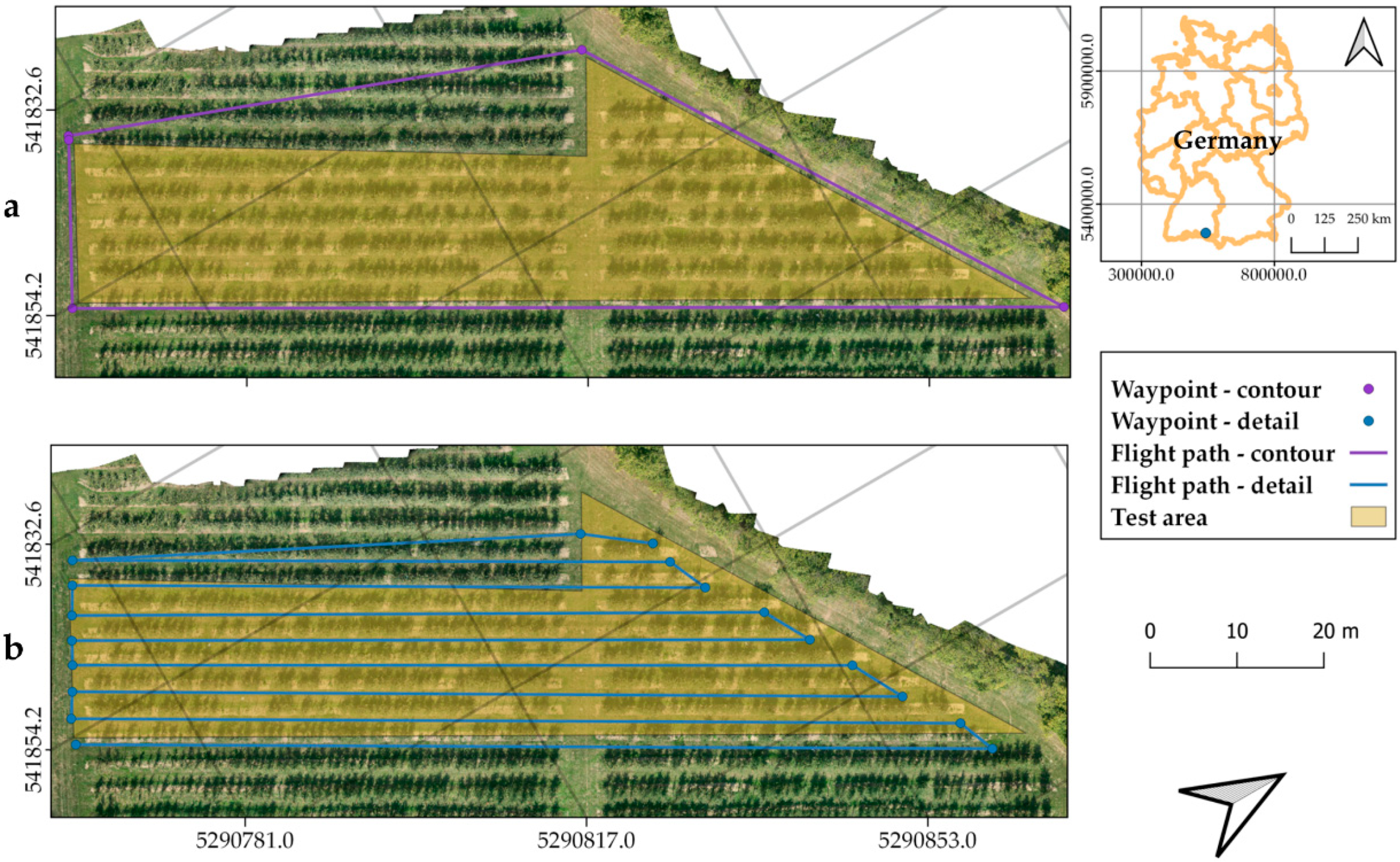
Two flight patterns were used for each date, as depicted in
Figure 1: an overview flight (
Figure 1a) and a detailed flight (
Figure 1b). During the overview flight, the orchard was captured from a larger perspective over its boundaries. The UAV circled along the contour of the orchard at an altitude of 20 m and images were taken with an angle of 9° against nadir. The resulting sampling distance (SD) on the tree wall surface was about 4.63 mm for the first captured tree row. SD is comparable to the ground sample distance but calculated for the vertical tree wall surface at a tree height of 1.5 m above ground level. The detailed flight was conducted directly afterwards, with a flight altitude of 10 m. The flight path followed the tree rows while the camera took oblique shots with an angle of 20° against nadir. In that way, a clear view of the neighboring tree row was achieved. The resulting SD of the depicted neighboring tree row was 2.25 mm. The flight speed was set to 1 m/s, which resulted in a forward image overlap of 92% and 85% on the first depicted tree wall for the contour and detailed flight, respectively.
For georeferencing and to combine several point clouds, marker plates were visibly placed within the orchard. The coordinates of each plate were recorded using a GNSS-RTK system (HIPer Pro, Topcon, Tokyo, Japan). The coordinates were stored in the WGS84 (EPSG: 4326) coordinate system and later transformed to the ETRS89 UTM zone 32N (EPSG: 25832) coordinate system.
2.3. Ground-Based Reference Measurements
LiDAR reference measurements were completed with an LD MRS 400001 (Sick, Germany) on the same date as the UAV flights. The monochromatic outdoor laser scanner had a size of 94 mm × 165 mm × 88 mm. It was set to an opening angle of 110° with an angle resolution of 0.25°, which allowed working from a minimal distance of 0.5 m. The LiDAR sensor was mounted vertically on a tractor 2 m above the ground with a preset angle of 0° and a measurement frequency of 25 Hz. The tree rows were scanned highly accurately at a slow driving speed of about 0.4 m/s. The resulting scan resolution alongside the tree row was 16 mm. Each tree row was scanned from both sides.
2.4. Data Analysis
The images of each flight campaign were photogrammetrically processed (Metashape, Agisoft LLC, Russia) to estimate the 3D point clouds. The software used SfM and multi-view stereo reconstruction. Parameters for calculating the image position as well as its orientation and matching with overlapping neighboring images were set to high quality. To improve the quality of dense cloud reconstruction, the sparse cloud was manually processed. The elimination of particular points was achieved by setting thresholds for reprojection error, reconstruction uncertainty, and projection accuracy to maximum values of 0.1, 50, and 10 pixels, respectively. Calculated image positions, orientations, and matches were updated based on the remaining tie points. The reconstruction of the dense 3D point cloud was set to “high” quality and “mild” depth filtering. The calculation time to compute the point clouds from the aligned 546 and 578 photographs took about 83 and 200 min for 2018 and 2019, respectively. Finally, the resulting 3D point clouds were georeferenced into the ETRS89 UTM zone 32N (EPSG: 25832) coordinate system and the tree rows were cut out.
The LiDAR data were recorded by self-written software that visualizes the actual scanner data on the vehicle for testing purposes and simultaneously saves the data in a self-written binary format (.sld) for further processing. This consists of an identification char-array of 14 bytes, followed by a binary header with information of the LiDAR scanner, number of scan points per rotation, and number of total scans. Attached to this header, all data of the scanned points are also saved in binary format.
To obtain the necessary point cloud reconstruction from the LiDAR data, a basic coordinate transformation for the given 2D-LiDAR was completed by an evaluation script (.m) programmed in MatLab (version 2018a or 2019a depending on the year of measurement; Mathworks, USA). The moving direction of the vehicle on which the LiDAR was mounted is represented on the x-axis. The y- and z-axes correspond to tree height and distance between sensor and tree row. The latter values are based on the time of flight of the laser impulse and the mirror angle. As the LiDAR instrument has a fixed position on the vehicle, a reference to new x, y, z coordinates was calculated from each echo position. The exact procedure is described in more detail in Dworak et al. [
49]. The calculated LiDAR point cloud is oriented in a local but metric coordinate system.
The two point clouds, one for each side of the tree row, were then merged to form a unique point cloud for a single row. The alignment was completed with the maximum cover ratio function using CloudCompare software [
50]. The prerequisite was manual selection of 10 arbitrary matching points in the two point clouds opposing each other. The automatic matching of the point clouds was completed with a root mean square difference of 0.00001 m to yield exact matched clouds. Furthermore, a targeted overlap of 90% was set because the viewpoint of the LiDAR sensor was different, so the point clouds did not entirely show the same objects. To diminish the influence of driving speed on the LiDAR point clouds, subparts along the tree row were aligned separately. In addition, obvious noise points were manually cleaned from the reference data. The combined point cloud was then scaled in the x and y axes to the extensions of the already georeferenced UAV point cloud. The height was not scaled. The LiDAR point cloud was then translated and rotated to align to the coordinate system and to the orientation of the UAV point clouds. After registration, points representing hail net poles or single plant growth rods in both the UAV and LiDAR point clouds were deleted so that only the trees and the orchard ground were part of the point clouds.
In the next step, the distances between tree points to the immediate ground were calculated using R-script [
51]. For this, the point clouds were first classified using the cloth simulation filter according to Zhang et al. [
52] with the lidR-package [
53] into tree and ground points. The parameter rigidity and cloth resolution were set to a value of 0.5 and the slope parameter to a value of 1. A constant threshold of 0.25 m was used as the distance to the simulated cloth to discriminate a point cloud into ground and non-ground classes. With these settings, adequate separation between tree and ground points except for small tree stumps was achieved. To remove the effect of the tree stumps and yield an even reference surface, a plane was estimated within the ground point cloud using a local linear regression model with the loess function [
50]. Only a small degree of smoothing of the model was used by setting the span parameter to 0.3. The predicted grid surface had a resolution of 0.01 m. This surface was used as the ground base surface. As a final step, the distances between the tree points and the nearest point on the ground base surface were calculated, constituting the height of the tree point over the surface. These distances were found by using a nearest neighbor approach based on a KD-tree search algorithm for 3D coordinates. The calculation was implemented in the R package “Rvcg” (modified from Schlager [
54]). Tree point distances were calculated for both UAV and LiDAR point clouds.
All tree point heights from the point clouds were then summarized along a 0.25 m georeferenced grid positioned along the tree rows by finding the maximum tree point distance in each grid cell using QGIS [
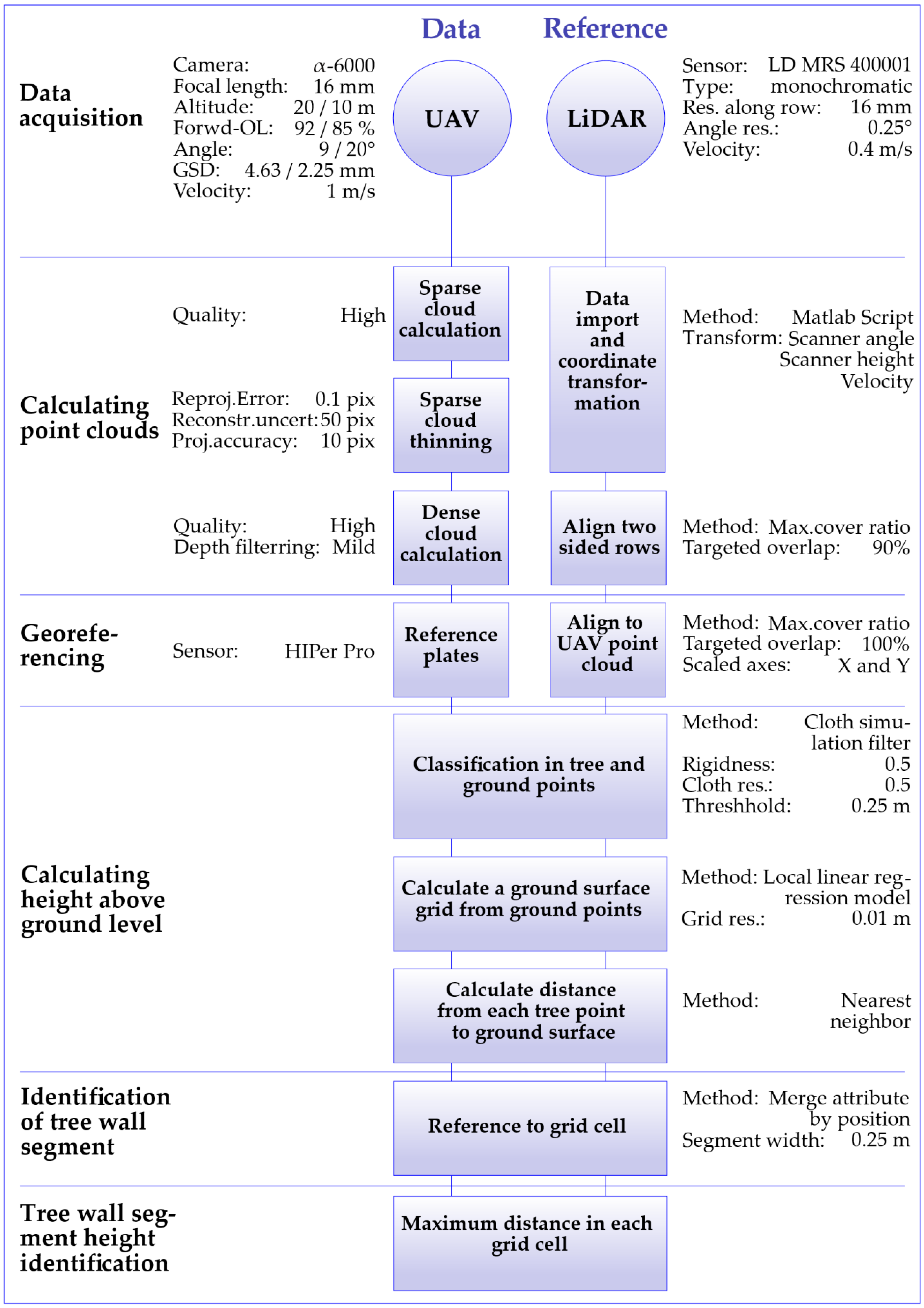
55]. For this, each tree point height was perpendicularly projected into the grid cell by the merge attributes by position function. All points of the same cell got an identifier (ID) for labelling. For estimation of tree wall height per cell, the maximum value of z-coordinates was retrieved and stored for each point cloud. This way the contour of the tree wall as calculated from the UAV and LiDAR point cloud could be retrieved in a spatial resolution of 0.25 m. An overview of the whole data processing is shown in
Figure 2.
To estimate UAV point cloud quality, different quality parameters were calculated for the separate tree points of each tree row using CloudCompare software [
50]. The point cloud density was determined volumetrically with a next-neighbor approach. For this purpose, the number of neighboring points within a sphere of 1 m
3 (r = 0.620 m) was counted and averaged for each point in the cloud. To determine the point cloud completeness, a two-dimensional grid with squared cells and a width of 0.1 m was created in nadir perspective with the same software. This was carried out individually for all rows. The result is shown as the relative proportion of filled cells in the UAV point clouds compared to the filled cells of the LiDAR reference.
The tree wall contours of the UAV point clouds were compared with the contours of the LiDAR reference measurements. To compare the maximum height of each grid cell between UAV and LiDAR data, mean error (
ME) for bias, mean absolute error (
MAE) for accuracy, and the correlation-based performance parameter coefficient of determination were calculated as follows:
where U and L denote the contour heights of the tree wall calculated from the UAV and LiDAR point clouds. The comparison was carried out for each tree row separately and for all data pooled together.
To analyze the UAV point clouds for missing branches, the function cloud-to-cloud distance in CloudCompare [
50] was used to calculate the point cloud distance. Here the distance from each point to the nearest point in a reference point cloud is calculated. For this analysis the LiDAR point cloud was compared to the UAV reference. In that way, points in the LiDAR cloud representing branches, which are missing in the UAV cloud, show further distance from their nearest neighbor. The result is a point cloud in which the distance to the reference point cloud of each point is displayed by a color scale. Thus, missing branches in the reference point cloud are highlighted. This analysis was completed for the years 2018 and 2019 individually. To keep the results comparable, the octree level setting, the level of subdivision of cubic volumes into which the cloud is divided, was kept stable at 10 for both calculations. To detect underestimated areas in the UAV point cloud, all points with a distance value of more than 0.2 m were extracted from these point clouds. The resulting sub point cloud was analyzed with the method Label Connected Components in the software CloudCompare [
50]. A minimum cluster size of 30 points and a maximum distance of 48.6 mm between the points were set to filter single points. The combined clusters were counted and evaluated for the years 2018 and 2019, respectively.
3. Results
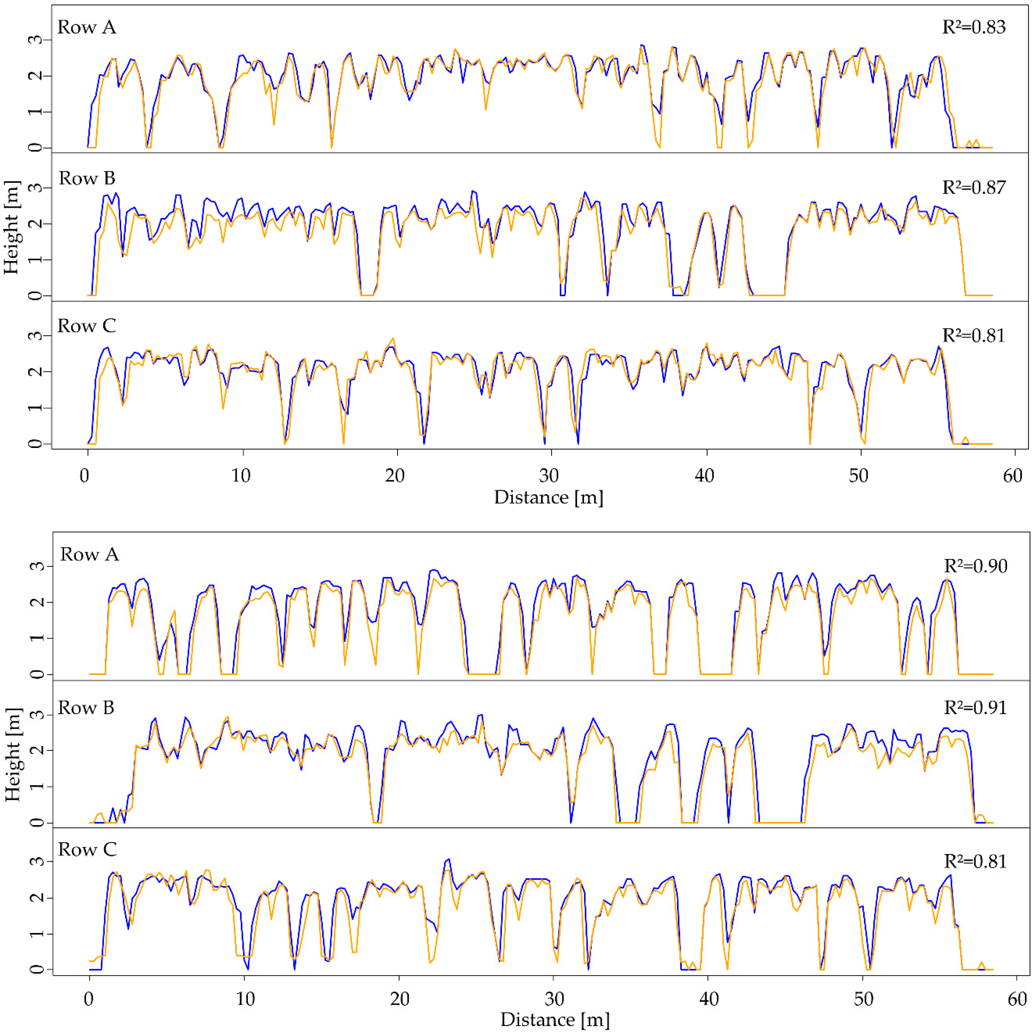
Figure 3 shows a comparison of UAV and LiDAR point clouds for the three apple tree rows A, B, and C for the years 2018 and 2019. The lines show the interpolated values of the maximum tree wall heights as found in each 0.25 m grid cell along the tree rows for both point clouds.
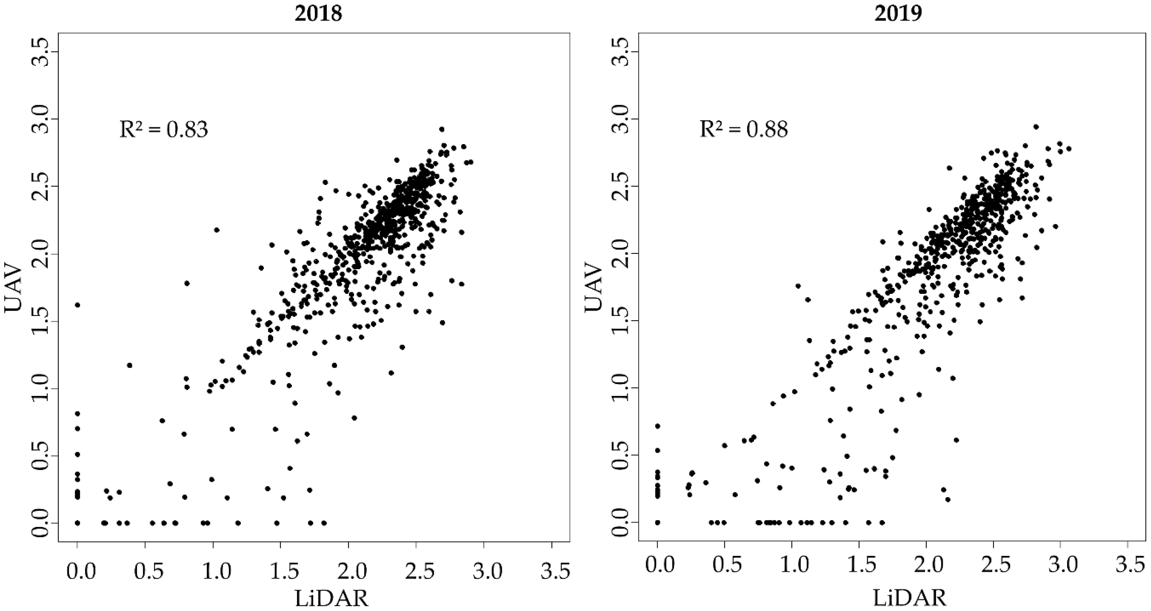
All contour curves for the tree rows showed high correlations for both tested years, as can also be seen from the scatter plots in
Figure 4. The highest coefficients of determination between tree wall heights from the UAV and LiDAR point clouds were R
2 = 0.87 in 2018 and R
2 = 0.91 in 2019. However, we found two types of deviations between the two types of point clouds. First, along the tree groups, a general weak underestimation of the contour curves from the UAV point clouds is recognized, especially for row B in 2018, and a nearly constant underestimation for row A and B in 2019. Second, there is a deviation in the transition from tree groups to tree gaps, where the tree height curves show steep slopes. Even though the tree gap detection works well, the width of the tree gaps tends to be overestimated by the UAV point cloud model (e.g., row B in 2019 at a distance of 34–35 m or 42–45 m).
Table 1 shows a list of quality parameters of the UAV point clouds. The volumetric density of 3D points for one row in both years ranged between 4.5 × 10
5 and 5.1 × 10
5 points/m
3 for 2018 and from 3.8 × 10
5 to 4.4 × 10
5 points/m
3 for 2019. The top-down point cloud completeness ranged from 76.6% to 86.6% and 73.1% to 86.2% compared to the LiDAR reference clouds for 2018 and 2019, respectively. For 2018, the fewest points per grid cell, around 16.000 points, were found in row B, whereas for 2019, row A had the fewest with around 9000 points per grid cell. This is accompanied by stronger underestimations of tree wall heights compared to the reference. All UAV point clouds are significantly correlated with the LiDAR reference point clouds (Pearson p < 0.0001). For 2018, R
2 values ranged between 0.81 and 0.87, with a mean absolute error (MAE) between 0.18 m and 0.23 m. For 2019, R
2 values ranged between 0.81 and 0.91, with a mean absolute error between 0.21 m and 0.24 m. The MAE of the tree height estimations ranged from 12.5% to 15.3% and from 9.2% to 13.2% for 2018 and 2019, respectively. As recognized from
Figure 3, the UAV point clouds underestimated to some extent relative to the LiDAR reference model, on average, for the three rows and two years.
In
Figure 4, all tree height estimations are pooled within a scatter plot showing the UAV data compared with the LiDAR data. With R
2 values of 0.83 and 0.88 for 2018 and 2019, respectively, the estimated tree heights from the UAV model fit the reference model quite well. However, a general underestimation of the UAV point cloud leads to more right-shifted points. This effect is intensified by zero values in the UAV point cloud (17 and 21 of 706 data points in 2018 and 2019, respectively), based on widened tree gaps. Additionally, there were some zero values in the reference cloud (14 and 18 of 706 data points), where noisy points in the UAV model led to tree height estimations.
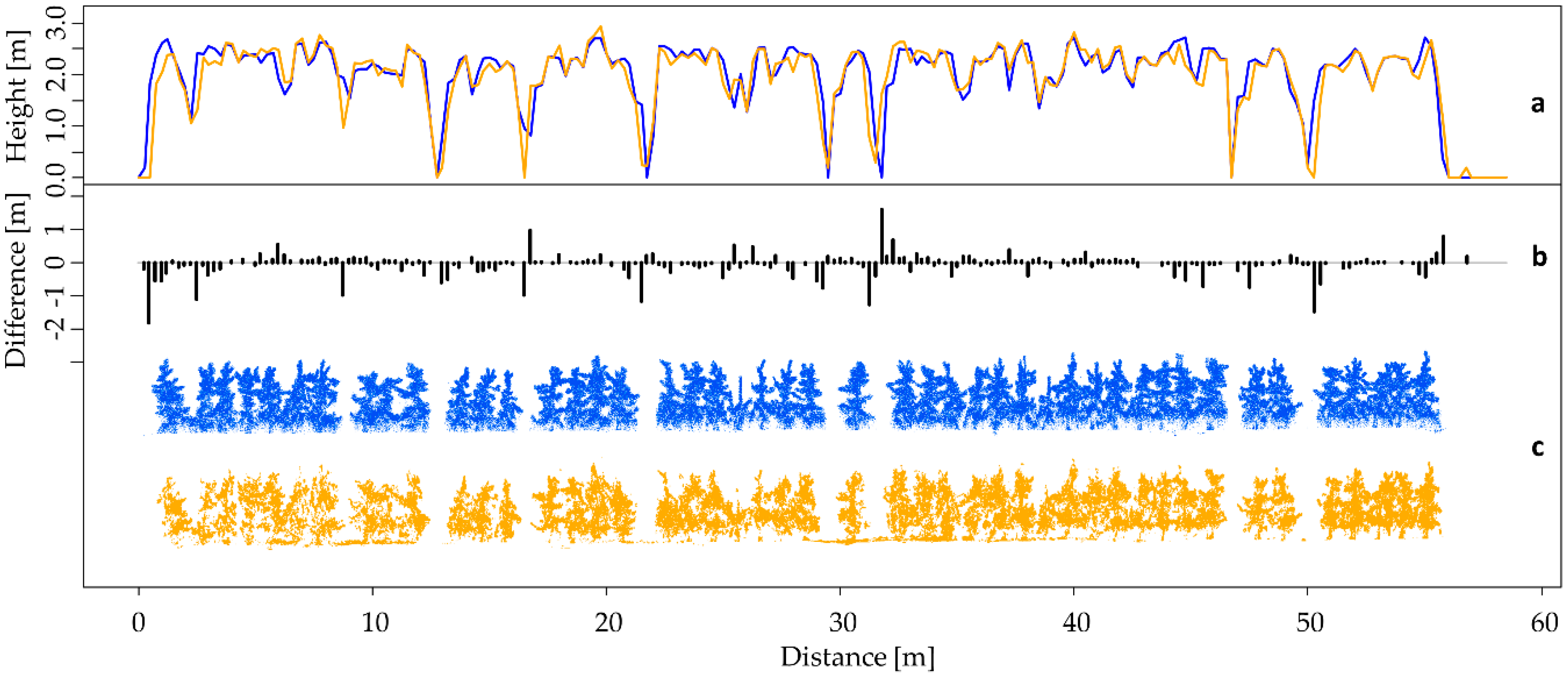
In
Figure 5, a more detailed comparison of the UAV and LiDAR point clouds for row C in 2018 is shown (
Figure 5c). As shown before, the general structures are mapped accurately from the UAV point cloud, e.g., tree profiles and gaps. However, the LiDAR data allows for more details and characteristics of the apple trees, although it has fewer points. The LiDAR point cloud even rendered fine shoots of the trees. For the UAV point cloud, it is noticeable that points are not as homogenously distributed over the row as reference points. In the example, the last tree group (distance > 50 m) shows structural quality that is visually about the same as in the reference cloud, whereas the first tree group (distance < 10 m) shows a more porous profile in the UAV point cloud. However, despite the heterogeneous point distribution in the UAV point cloud, the delineated tree heights were hardly affected (
Figure 5a). The bar plot in
Figure 5b shows the differences in maximum tree wall height estimations from both models. In general, the differences are rather small, with a tendency to underestimate the LiDAR tree wall height references to some extent. When comparing the two point clouds, this comes from the SfM approach missing fine structures of tree walls, such as small shoots in the upper part of the trees. Larger deviations occur mainly in the vicinity of tree gaps in areas of steep slopes of the tree height curves. Here, widened gaps in the UAV point cloud cause strong differences in height estimation. This happens because fine lateral shoots are estimated shorter and therefore a gap is detected instead of the tree height value. This increases the underestimation effect of tree height estimates by the UAV point cloud.
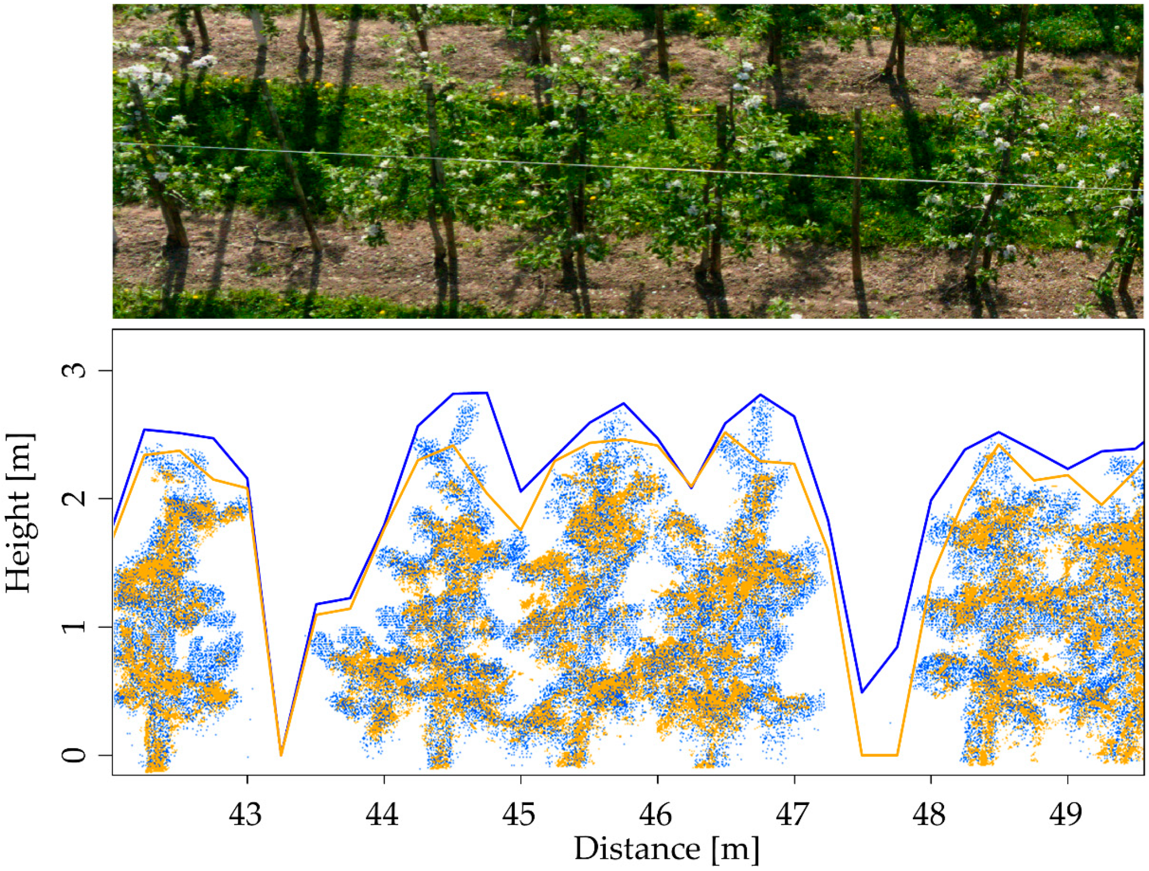
To visualize this effect in more detail,
Figure 6 shows RGB images shot from the UAV and the calculated UAV point cloud superimposed with the reference LiDAR point cloud for five trees as an example. We see that the orange UAV point cloud outlines a good tree crown profile but fewer details in the structures at the crown edges compared to the reference LiDAR point cloud, depicted here with blue points. Due to the lack of fine shoots in the UAV point cloud, the lateral and vertical expanses of the apple tree canopies were attenuated. In the detailed view for tree wall contour curves, this leads to an underestimation of all tree crown maxima, especially within the canopy gaps and at the beginning and end of tree groups.
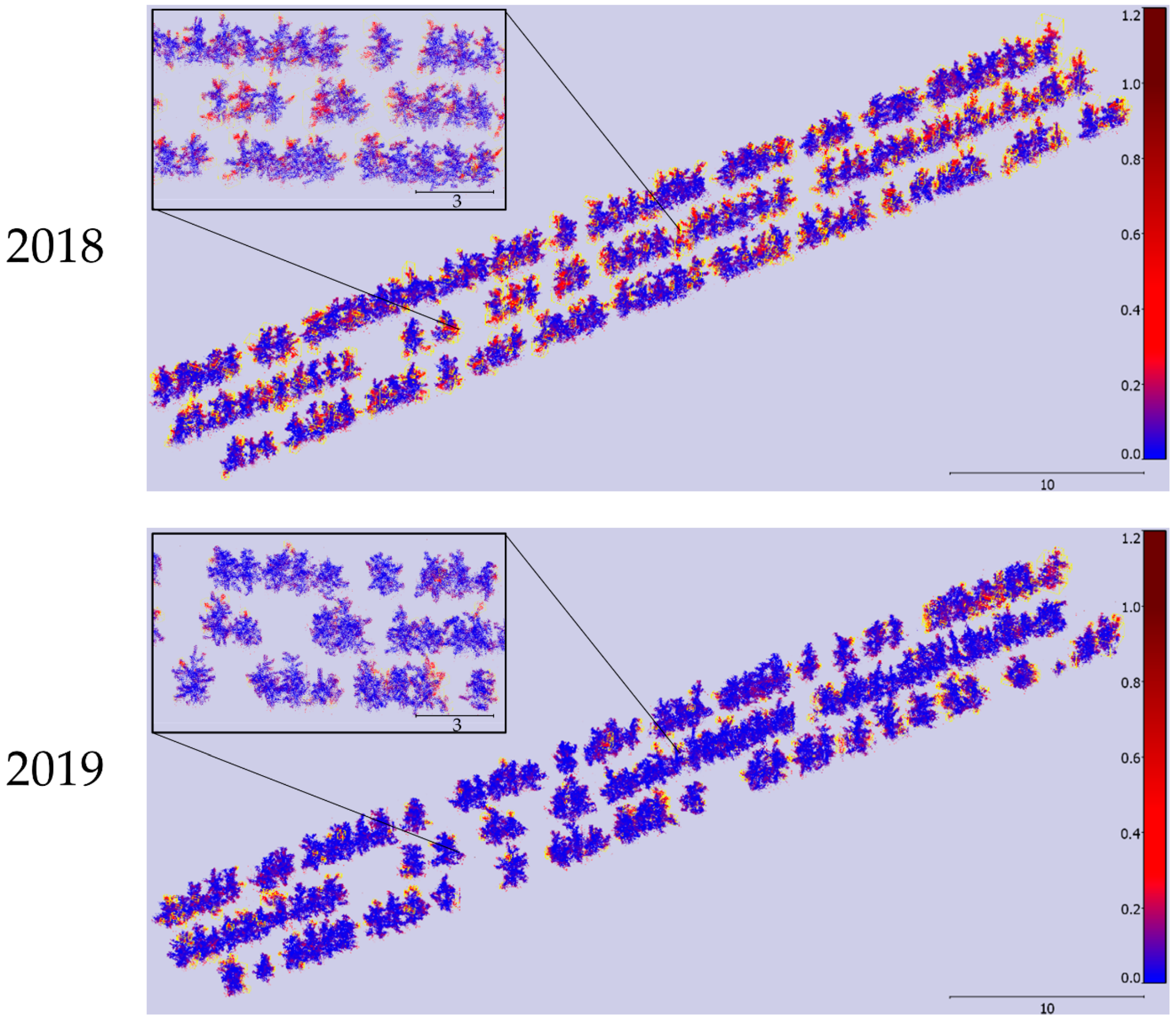
To show the effect of underestimated areas, which are often missing branches, over the whole orchard,
Figure 7 displays an overview of the distance of each point to its nearest neighbor in the compared cloud. Here, the LiDAR point cloud shows all small shoots. In that way, points representing branches that do not exist in the UAV point cloud are further away from their next neighbor and are therefore highlighted in red. The blue center of the trees can be seen over the whole orchard for both years. Therefore, tree structures in general are well represented in the UAV point clouds. However, red clusters at the top of the trees and in the transition from gap to tree group indicate problems with the UAV point cloud in depicting these finer structures. This becomes particularly clear in the magnified areas of the tree rows. Missing point cloud clusters, which are framed with yellow boxes, are located around the tree. Here, as already described, missed fine shoots lead to an underestimation of tree height and to a widening of tree gaps. Over the orchard 555 and 299 missing point cloud clusters were identified for 2018 and 2019, respectively. It is assumed that different recording conditions, such as different wind conditions, led to the variation in quality of point cloud delineation for small branches.
4. Discussion
To meet the requirement for more detailed information in modern precision horticulture, UAV-based measurements deliver interesting new data. The experiments carried out within the present framework used low-altitude flights. A consumer grade camera system together with modified photogrammetry methods were used to determine the height of apple fruit tree wall sections. The results are based on data from flight campaigns of two years in which three apple tree rows, consisting of 168 individuals, were mapped. The comparison of tree wall heights delineated from UAV and reference LiDAR point clouds shows that low-altitude UAV imagery is appropriate to systematically observe apple tree growth within the tree wall sections of orchards.
The correlations found in this study for tree height estimations from UAV point cloud and reference data were comparable with results obtained for olive tree plantations by Diaz-Varela [
47], where the root mean squared errors ranged between 6% and 20%. Slightly minor errors between 3.5% and 3.8% were stated by Torres-Sánchez et al. [
48] for large olive tree walls, corresponding to a difference of 0.17 m and 0.18 m. In comparison, we found slightly higher errors ranging from 0.18 m to 0.24 m in our study.
The studies mentioned above used high flight altitudes for nadir UAV measurement campaigns to delineate structural parameters from trees. This way, there can be high image overlap, from which the SfM photogrammetry benefits. This was the same in the case of Dandois et al. [
56], who found that a high forward overlap of UAV imagery from 60% to 96% is crucial for minimizing the canopy height error for forest point clouds. Torres-Sánchez et al. [
46] came to a similar conclusion. They found that a forward overlap of 95% was appropriate for 3D surface modelling of orchard trees with regard to processing time and flight time. All of these studies used higher flight altitudes than in our case, and therefore benefited from larger ground area covered by each image. Therefore, the trade-off between image overlap and flight time is not as crucial as it is for low-altitude UAV imagery. This way, however, they lose details due to greater ground surface distance.
However, with further advancement in battery technology, flight time limitations will become more negligible, so that a high percentage of image overlap can be combined with low-altitude flights. Seifert et al. [
57] found that this would give the best reconstruction quality for forest trees. As a reasonable amount of forward overlap for low flight altitudes, taking processing time as a practical limitation factor, the authors suggested 95% [
57].
For oblique image flight campaigns in orchards, the target area from which image data should be acquired with high overlap should be the tree wall area to receive maximum information. For this study, flight patterns were set in a way that the forward overlap in images along the tree wall was about 85% due to the low flight velocity of 1 m/s. For more stable point cloud calculation, the flight velocity might be decreased even further. In that way, areas with lower point density in the point clouds would be prevented from reducing the underestimation of crown height. This is reasonable, because regions in a point cloud that have fewer points compared to their surroundings might suffer from greater uncertainty in 3D point cloud reconstruction. Therefore, it will be even less probable that finer structures will be found in the UAV point cloud. Therefore, these areas are strongly underestimated. It is shown that even poorly resolved tree wall sections in a UAV point cloud can lead to stable but underestimated height information.
A major struggle for the UAV photogrammetry in our study was the estimation of fine shoots, which develop after the slender apple spindles in the tree walls are pruned each year. We found 555 and 299 missing point clusters, which are interpreted as missing shoots, over the orchard for 2018 and 2019, respectively. These small structures had very low color contrast against the background, which is a common problem for small apple orchards [
58], and spanned only a small area in the photographs. This makes the distinction between foreground and background challenging [
59]. In addition, small branches can easily move in the wind by multiples of their own diameter. These problems make the SfM approach struggle when estimating accurate point locations for fine structures in dense clouds. This is consistent with other research findings. Fritz et al. [
60] found that thinner branches in SfM based point clouds from non-nadir forest overflights remain likely to be undetected. They concluded that a systematic underestimation of tree row heights can hardly be prevented. For our study, this underestimation occurred mainly in two ways. On the one hand, lower crown heights were estimated where thin branches in the upper part of the trees were missing. This effect was generally observed for most of the tree tops along the apple tree rows. On the other hand, small twigs, hanging laterally in the tree wall gaps, often could not be found. This effect occurs around tree gaps, widening them in the UAV point cloud. Therefore, underestimations of the tree wall heights occur with the SfM approach at the beginning and the end of tree groups. To cope with this problem for crop protection, e.g., application maps for spraying measures, a buffer could be used over the tree contour line. Based on the findings of underestimation in our study, we would suggest a buffer size of about 20 cm.
When calculating three-dimensional point clouds from images, tree parts can be missed, for which no sufficient two-dimensional data are provided. Frey et al. [
61] compared the amount of three-dimensional grid cells, or voxels, containing points in the three-dimensional space in relation to their most filled model when working with a UAV based SfM approach in forests; they call it digital surface model completeness. They found a positive correlation between GSD and the completeness of surface models for two-dimensional ground surface, but this correlation disappeared for the three-dimensional voxel space. They concluded that fine GSD and high image overlap are both beneficial for sampling lower tree canopy parts. In our study, we used a small surface sampling distance, which resulted in good model completeness values ranging from 73.1% to 86.6%. However, image overlap has a stronger effect on 3D model completeness, as Frey added. Therefore, the problems in reconstructing small shoots in UAV point clouds should be addressed using slower flight speeds, with consequent higher image overlaps. In summary, it is a trade-off between the level of detail in the point clouds and the processing time. For coarse structure delineation, high flight altitude and a fast point cloud processing would be sufficient, while tasks such as site-specific plant protection and yield estimation would benefit from a higher level of detail. For these applications, a maximized crown wall area in photographs taken at a low flight altitude and an oblique view combined with high forward overlap of images is recommended.


