Article

Improving the Accuracy of Automatic Reconstruction of 3D Complex Buildings Models from Airborne Lidar Point Clouds

by
Marek Kulawiak
* and
Zbigniew Lubniewski
Department of Geoinformatics, Faculty of Electronics, Telecommunications and Informatics, Gdansk University of Technology, 80-233 Gdansk, Poland
*
Author to whom correspondence should be addressed.
Remote Sens. 2020, 12(10), 1643; https://doi.org/10.3390/rs12101643
Submission received: 8 April 2020 / Revised: 7 May 2020 / Accepted: 14 May 2020 / Published: 20 May 2020
(This article belongs to the Special Issue 3D Urban Modeling by Fusion of Lidar Point Clouds and Optical Imagery)

Abstract

:
Due to high requirements of variety of 3D spatial data applications with respect to data amount and quality, automatized, efficient and reliable data acquisition and preprocessing methods are needed. The use of photogrammetry techniques—as well as the light detection and ranging (LiDAR) automatic scanners—are among attractive solutions. However, measurement data are in the form of unorganized point clouds, usually requiring transformation to higher order 3D models based on polygons or polyhedral surfaces, which is not a trivial process. The study presents a newly developed algorithm for correcting 3D point cloud data from airborne LiDAR surveys of regular 3D buildings. The proposed approach assumes the application of a sequence of operations resulting in 3D rasterization, i.e., creation and processing of a 3D regular grid representation of an object, prior to applying a regular Poisson surface reconstruction method. In order to verify the accuracy and quality of reconstructed objects for quantitative comparison with the obtained 3D models, high-quality ground truth models were used in the form of the meshes constructed from photogrammetric measurements and manually made using buildings architectural plans. The presented results show that applying the proposed algorithm positively influences the quality of the results and can be used in combination with existing surface reconstruction methods in order to generate more detailed 3D models from LiDAR scanning.

1. Introduction

Acquisition of the detailed, three-dimensional spatial data describing accurately the terrain and topographic objects is an important problem due to a wide range of applications, including:
  • Creating detailed three-dimensional topographic maps;
  • Modeling of various processes and phenomena in relation to a given area [1,2];
  • Reproduction of detailed digital models depicting architectural monuments [3,4];
  • Numerous applications in geographic information systems (GIS) [5,6,7].
Due to the continuous increase of data amount used by applications such as those mentioned above and others, automatized, efficient and at the same time, reliable, spatial data acquisition methods are needed. A high level of accuracy and reliability characterizes manual measurements carried out by surveyors using traditional methods supported by very accurate differential GNSS receivers, but this approach to collecting data is very time-consuming and expensive. An alternative is the use of photogrammetry techniques, as well as mobile light detection and ranging (LiDAR) scanners as a source of information regarding terrain height and the shape of various objects [8]. The use of LiDAR technology, in particular, has become widespread, as it enables large-scale investigation of terrain and objects using a single device emitting a large number of beams [9,10,11].
Three-dimensional terrain data derived from a set of photogrammetric images or obtained by the process of laser scanning generally have the form of a set of discrete points, irregularly arranged in three-dimensional space, according to the shape of an investigated object. This form of data set is referred to as a point cloud [12] and it has known disadvantages as far as several applications and processing efficiency are concerned. In particular, some elements, such as small objects, may be difficult to distinguish in the data described by point clouds or pixels, as opposed to data represented by other geometrical structures, such as polygons or polyhedral surfaces, e.g., triangulated irregular networks (TIN [13]). In the case of data sets with low point density, their readability can only be ensured if they are observed from specific location and orientation of the acquisition device with respect to measured object. Moreover, point clouds obtained via photogrammetry and LiDAR surveys often are incomplete, which means that they do not cover the entire area of the scanned object in a uniform way. In the case of photogrammetry, this may be caused by occlusion of the scanned object by another entity or a lack of appropriate vantage point to capture the object in its entirety. As far as the airborne LiDAR is concerned as a data source, this is often caused by the particular angle at which the laser beam is directed towards the scanned object. An example of this issue is shown in Figure 1.
In the context of the above issues, spatial data obtained from these sources must be corrected and transformed into 3D object models represented by the appropriate format, e.g., TIN. This article presents an algorithm for correcting 3D point cloud data obtained from airborne LiDAR field surveys of regular 3D objects such as buildings. The proposed approach assumes the application of a sequence of operations resulting in 3D rasterization, i.e., creation of a 3D regular grid representation of an object, prior to applying the regular Poisson surface reconstruction method [14]. In order to verify the accuracy and quality of reconstructed objects, the reference models were used. For this purpose, the meshes constructed from the photogrammetric measurements, as well as made by hand on the basis of buildings architectural plans, were utilized.
Existing solutions for 3D reconstruction of objects shape from LiDAR data include approaches, such as assembling building blocks from a set of standard roof shapes stored in a database [15], roof plane segmentation performed by minimizing an energy function [16], merging LiDAR and hyperspectral image data and performing shape reconstruction using the implicit geometry method [10], decomposing building footprints and estimating roof models with the use of RANSAC technique [17], reconstructing building roofs from LiDAR data integrated with optical multi-view images [18], combining LiDAR point clouds with street view images by adopting rule-based parsing and boosted decision trees [19], preprocessing input data with the use of block partitioning and contour extraction [20], primitive clustering and boundary tracing of building rooftops [21], as well as applying building contouring algorithm to classified height maps [22]. An extensive review of the state-of-the-art in urban models’ construction from LiDAR point clouds—not only limited to buildings—is given in [23].
From a more detailed analysis of the state of the art, it may be concluded that the existing solutions are only partially satisfactory and still need extensive research. To date, a large number of algorithms dedicated to transforming point cloud data into more complex TIN models is known: Poisson surface reconstruction [14] including modifications, e.g., screened Poisson surface reconstruction [24], ball-pivoting algorithm [25], Delaunay triangulation [26] and power crust algorithm [27]. Unfortunately, due to the nature of data acquisition methods based on the use of technologies related to laser scanning, the results often are unsatisfactory when standard surface reconstruction techniques are applied [28]. Common problems encountered include significant amounts of noise (i.e., existence of large numbers of points in a dataset which should be excluded from further processing), frequent local lack of data, as well as strong variability of local point density and data accuracy throughout a single dataset. To some extent, the data in this form can be used in order to recreate the buildings models in some cases [29,30]. However, in the case of more complex and varied objects, obtaining satisfactory results is often much more difficult to achieve [31].
In this context, the new approach to reconstruction of 3D models of topographic objects proposed in this study seems to be promising in terms of potential to improve the overall accuracy of the results. The primary goal of the proposed method is to generate meshes which would represent the scanned objects as faithfully as possible in actual 3D, in contrast to approaches based on creating minimalistic meshes [22] or models limited to 2.5D [21]. It is also meant to be a robust method suitable for point clouds, such as airborne LiDAR data and is expected to create satisfactory results without the need of providing it with additional input data, unlike many other solutions [10,18,19]. The authors intent is to also make this method simple to implement and adapt to different scenarios, which means that it should not rely on complex solutions such as machine learning [29].

2. Spatial Data

The primary spatial data used in this investigation was the airborne LiDAR measurements data obtained from scanning the particular object, i.e., building. The data set has the form of unorganized 3D point clouds. As real measured data were not accessible for the authors in some investigated cases, a LiDAR data simulation procedure was applied. Other source data were used as reference models. The meshes created from photogrammetric measurements, as well as made by hand on the basis of buildings architectural plans, were used for this purpose. In the following subsections, the particular types of data utilized in this work are described.

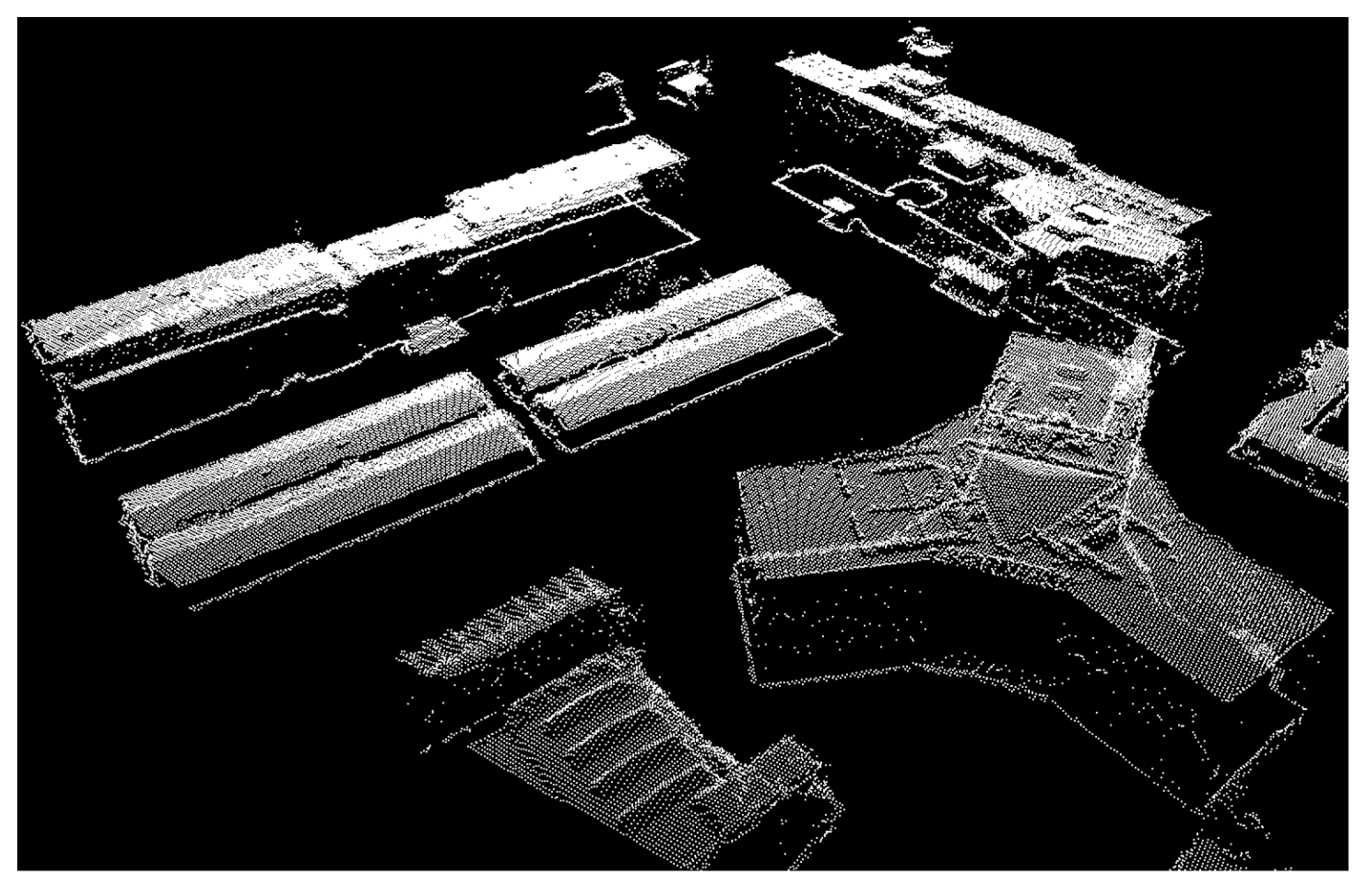
2.1. LiDAR Point Clouds

LiDAR data were obtained by laser scanning operation, which relies on emitting a laser beams in a large number of particular directions towards terrain or objects in order to determine the distance between the device and the terrain elements. Using the distance data along with the information on beams directions, the LiDAR software creates the 3D point cloud as the result.
In a mentioned case of airborne LiDAR scanning, the data were acquired using the vehicle flying above the scanned objects several times in different directions. It may be predicted that due to multiple measurements of the same object, the overall accuracy of data will be higher, but at the same time, disorder in data increases—a fact that must be taken into account in further processing.
LiDAR data were obtained from the Polish Center of Geodesic and Cartographic Documentation (GUGIK) [32]. The data set consists of airborne laser scans over several parts of Gdansk city area, Northern Poland and has the form of multiple LAS files (compliant with version 1.2 of the file format) with the average resolution of about 19 points/m2. The used LiDAR data set also contains additional information, such as the color value of every point, as well as classification information where each point in a cloud is assigned to a single class representing types such as buildings, ground, water and vegetation. This information was used supportively in extracting a particular subset, e.g., a given single building scan, from a scene.
The scans of particular buildings located in Gdansk area were selected for the tests of the proposed 3D shape reconstruction as described later in the study.

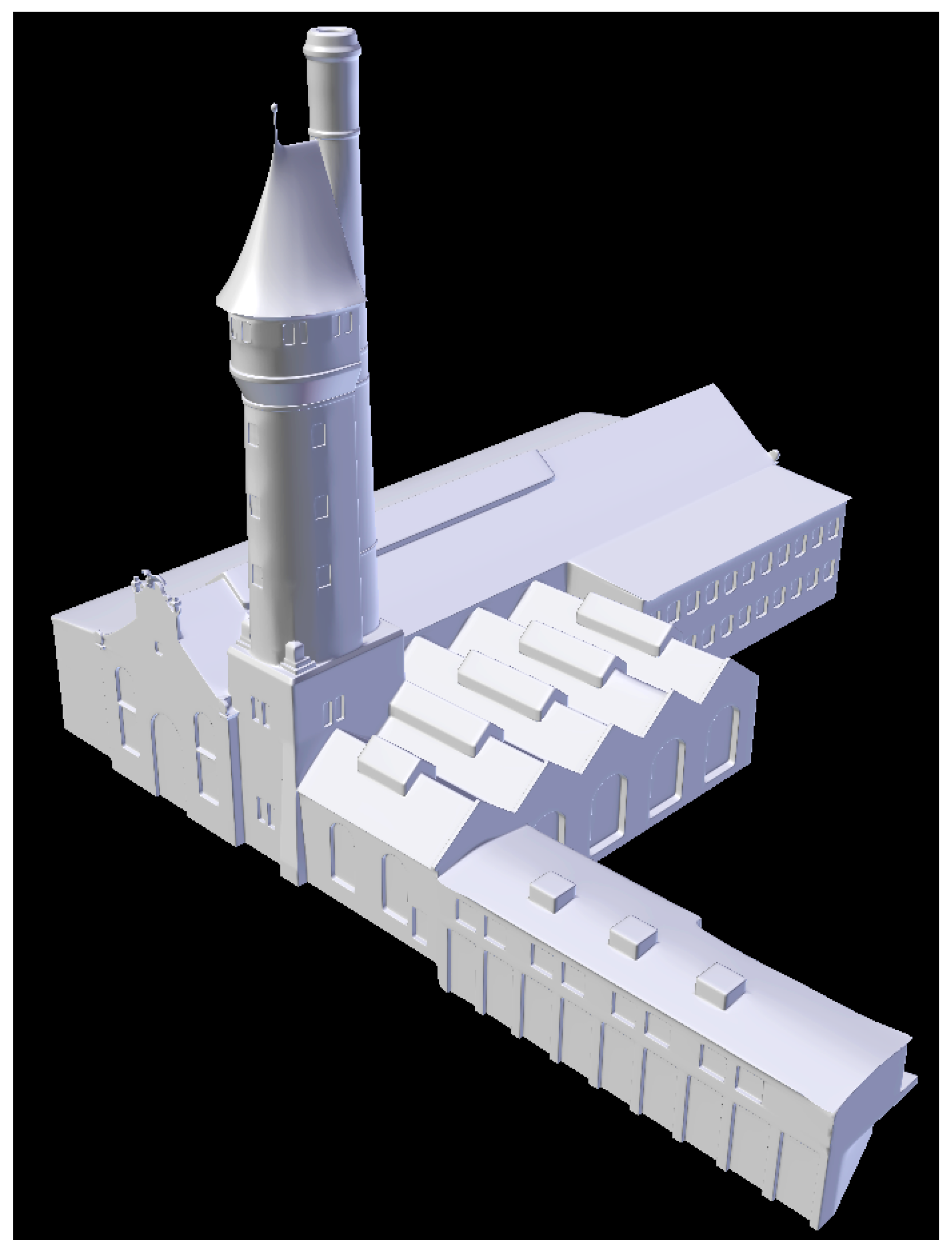
2.2. Reference Meshes
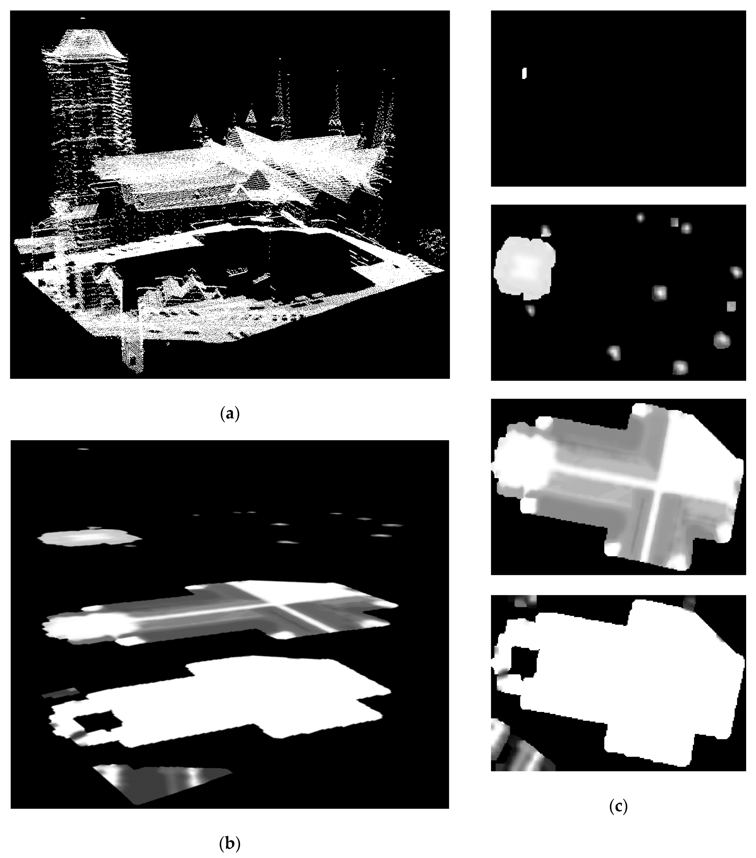
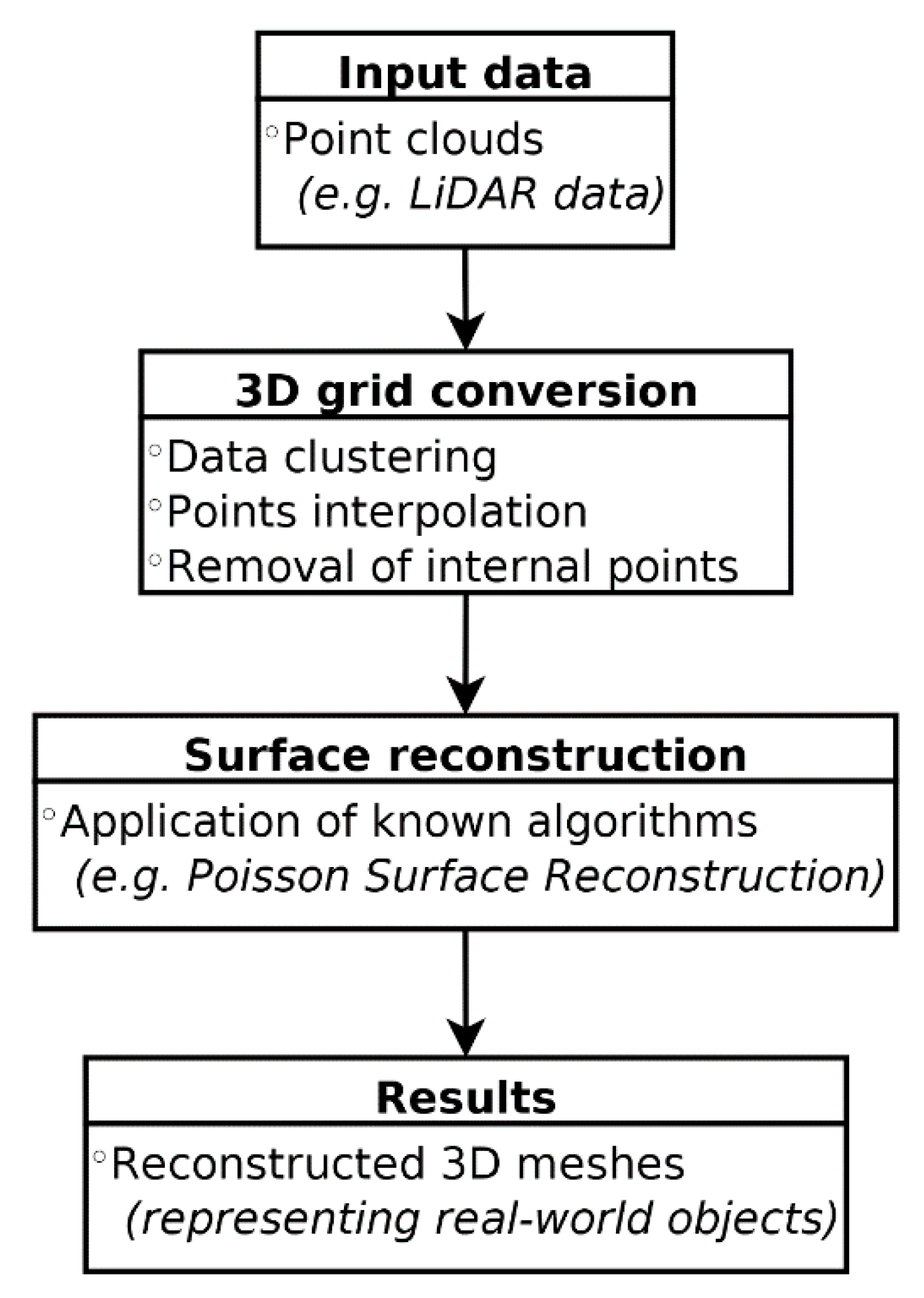
This section describes detailed three-dimensional meshes which are used as reference to verify the quality of output models obtained with the 3D grid reconstruction method.
The first reference mesh is a result of performing photogrammetric reconstruction based on a series of 323 photographs depicting the St. Mary’s Church in Gdansk. These photographs were taken at intervals of three to four meters in conditions of relatively uniform lighting. Then these photos were subjected to simple graphics processing performed in order to unify their level of brightness, contrast and sharpness, as well as rotating some of the photos. After processing, the photographs were provided as input of Agisoft PhotoScan 1.3.0, which was used to generate a complex point cloud and convert it into a textured mesh. Unfortunately, all the photos provided to the program were taken with the camera positioned at a height close to ground level, which resulted in inaccurate representation of the higher parts of the Church, which is over 80 m tall. Due to the above, the algorithms used by PhotoScan received too little information at the input, so the generated 3D mesh of the Basilica contained significant information deficiencies (“holes”) in the representation of the roof and numerous distortions on the surface of the towers. In addition, the resulting model also contained a large number of errors caused by obscuring the actual building by random objects, such as parked cars. In order for the obtained mesh to be successfully used for research, it was necessary to manually correct it in Blender 2.79b [33]. This correction included both removing the above-mentioned distortions and supplementing some elements of the model based on aerial photographs of the Church. The entire processing time took a total of over three weeks. The resulting model is presented in Figure 2.
The second reference mesh presents the Mechanical Laboratory building of the Faculty of Mechanics of Gdansk University of Technology. Initially, it was planned to use the same procedure for obtaining the mesh as in the case of St. Mary’s Church in Gdansk, however this approach was abandoned, as the building was obscured by too many elements of local topography of the area, which would undoubtedly disturb the process of photogrammetric reconstruction. Instead, the model was made by hand based on its architectural plans. This process took about three weeks, so it was similarly time-consuming, as the correction process of the generated model of St. Mary’s Church. The final version of the model is shown in Figure 3.
Since the processing methods for the first two reference meshes was very time-consuming, a different approach was used for other objects, somewhat inverse than above: instead of preparing reference meshes tailored to the needs of available materials regarding the results of LiDAR scanning, the existing building meshes were used, which were then provided as input to the process of simulated surface scanning. The simulation is designed to imitate the process of acquiring spatial data by a mobile LiDAR scanner located at a fixed height above the scanned object in three-dimensional space. The simulated scanner emits a set of rays in multiple directions, which are used for computing intersections with the object’s geometry. Finally, a point cloud is generated by inserting points at the places where the beam intersects with the given plane of the model [34]. The simulator application was created with the use of OGRE 2.0 [35], an open-source and cross-platform graphics rendering engine. A single surface scanning simulation is performed based on user-provided parameters, such as the number of rays emitted by the scanner, number of measurements (assuming a constant distance traveled between consecutive measurements), scanner initial position and heading, as well as maximum angle of ray deviation from the vertical plane. The application does not simulate LiDAR measurement noise, however its results were compared with LiDAR point clouds provided by GUGIK [32] for the area of Tricity in Northern Poland and the spatial characteristics of the generated point clouds were similar to actual scanning data. Since the simulation process allows obtaining reliable test materials in the form of point clouds from any three-dimensional meshes, this study is limited to describing only one test case: a simplified model of Castel Sant’Angelo in Rome, which was downloaded from the 3D Warehouse [36] and scaled to real-world dimensions. The building is 48 m tall and the simulation was used to imitate a multibeam laser scanner moving along two different tracks at a fixed altitude of 150 m above the ground level. In this case, a total of 200 simulated measurements were performed, with the distance between consecutive measurements equal to 125 cm, and the maximum angle of ray deviation was set to 100 degrees.

3. The Algorithm

The presented point cloud densification and reconstruction algorithm was created for correcting incomplete point cloud datasets obtained via field surveys of regular 3D objects. For the purpose of shape extraction and error correction, the algorithm uses a method of converting irregular point cloud data into a regular three-dimensional grid of points. The 3D grid can be interpreted as a set of overlaid 2D matrices forming a 3D shape, where each layer corresponds to a certain height, as shown in Figure 4. Each raster corresponds to a certain height range, where the pixel value represents its position on the vertical axis within this layer: small values (dark colors) represent the lower parts of a given interval, and large values (light shades) represent its upper ranges.
The pipeline of the proposed data processing method is shown in Figure 5. The 3D grid conversion algorithm involves several operations, including (but not limited to):
  • Clustering of input data by assigning every point to a single sector of a regular three-dimensional array. Each sector corresponds to an area in space represented by a cuboid;
  • Interpolating new points inside empty sectors if there are any other points nearby;
  • Removing any internal points of the object and leaving only those that represent the outer boundaries of the object.
The detailed behavior of the algorithm is strongly dependent on the processed data as well as operational environment parameters. During the first stage of operation, which involves data clustering, the most important parameter of the algorithm is spatial resolution of a single sector along the X, Y and Z axes (corresponding to width, length and height expressed in meters). Based on the given resolution, the input space of the point cloud is projected onto a set of three-dimensional sectors, the number of which along each axis is calculated according to the formulas presented in (1) and rounded to integers.
nx = Δx/rx
ny = Δy/ry
nz = Δz/rz
where:
nx, ny, nz—number of sectors in axis X, Y and Z,
Δx, Δy, Δz—width of the data ranges (distance between two the most extreme positions along a given axis),
rx, ry, rz—width, length and height of a single sector, expressed in meters.
In addition, the algorithm provides a set of optional parameters the proper use of which can positively affect the final processing result. The following parameters are available:
  • The hybrid mode option, which combines the generated set of points with the original input point cloud. Using this option reduces the regularity level of the resulting data set, but allows to more accurately reproduce the characteristic elements found in the original data;
  • Option to fill empty set elements within a single grid level. Enabling this option will fill in individual empty sectors based on data from its nearest neighbors;
  • The level of filling the empty elements between each level of the grid. This action is aimed at reducing the number of “holes” located in planes perpendicular to the ground. At each level of the grid, in order from lowest to highest, all empty points are searched and then for each of them the closest non-empty point directly above it (along the Z axis) is found. If the distance between these points does not exceed a certain value, then the value of the empty point is replaced by the value of the point directly above it. Passing this parameter to the input of the algorithm in many cases allows to supplement a significant part of the surface of the vertical walls, but in rare cases it can also generate new points in spaces that should remain empty, e.g., when the point cloud represents an object containing horizontal elements protruding above ground surface;
  • The intensity of the filtration used to mitigate the large differences in values between adjacent sectors at different levels of the grid. The value of this parameter is used to create a kernel for the simple low-pass filter, both dimensions of which are calculated according to (2). For each processed sector, its new height is set by this lowpass filtration to the value of the sum of its height and the height of its neighbors, divided by the number of sectors included in the calculation. This filtration is useful in situations where the data contains sets of irregularly distributed points representing oblique surfaces, such as roofs of buildings. Naturally, setting the blur_level parameter to 1 will result in using a 3×3 kernel, which is often considered as a minimum size in computer graphics.
dimension = 2 blur_level + 1
The next step of the algorithm involves interpolation of new points in the empty sectors of the 3D grid. This is realized by identifying the discontinuities in the outline of the 3D object and filling the appropriate sectors with new points whose values are extrapolated from the known values of the neighboring sectors in the 3D space.
While the processing resolution has the greatest impact on algorithm performance, other parameters can positively influence the quality of the processing results. These include:
  • Output hybridization, which merges the generated set of points with the original input point cloud. Using this parameter reduces the level of regularity of the resulting data set, but allows for a more accurate mapping of certain characteristic elements appearing in the original data;
  • Reconstructing empty elements in the set within a single grid level. Using this parameter populates individual empty sectors based on data from its nearest neighbors;
  • The level range at which empty elements of the point cloud are reconstructed between individual levels of the grid. This action is aimed at reducing the number of missing points of data in planes perpendicular to the ground. At each level of the grid, in the order from the lowest to the highest, all empty spaces are identified and then for each of them the nearest existing points in the vertical plane are found. If the distance between these points does not exceed a certain value, then the empty space is replaced by a value interpolated between those points;
  • Filtering intensity used to alleviate large differences in value between adjacent sectors at different levels of the grid. The value of this parameter is used to create a matrix for the needs of a simple low-pass filter. This filtration is useful when a processed set of points contains groups of irregularly distributed points representing oblique surfaces such as building roofs.
As the resulting dataset should consist only of points representing the external boundaries of a given object, such as walls or roofs of buildings, the final step of the algorithm involves the removal of any internal points the dataset may contain. For this reason, the following steps are performed as part of this conversion stage:
  • First, an auxiliary sector classification is created, dividing the set into two classes, describing the empty and filled sectors, respectively;
  • Then a new class is introduced, representing the edges of the outer surfaces containing filled sectors which are directly adjacent to empty sectors. As a result of this operation, the newly created class will represent the edge points of the object.
  • Finally, all points that are not classified as edge points are removed from the highest level in the set. In addition, points that have not been previously classified as edge points are removed from the remaining levels if other points exist directly above them (in an adjacent level).
When applied to incomplete point cloud data obtained from field surveys, the algorithm is capable of filtering out errors and recovering missing elements of the scanned 3D object. An example of the algorithm processing results is shown in Figure 6. The resulting regularized point cloud may be then used for the purpose of 3D shape reconstruction via algorithms such as the Poisson surface reconstruction [14].
In theory, the 3D grid conversion can be used with any shape reconstruction algorithm, although in overall the best results can be obtained using the traditional Poisson surface reconstruction method [14]. The extended version of this method, the screened Poisson surface reconstruction [24], can also be used, however it can cause excessive sharpening of mesh details even when using the minimum interpolation weight value. This can be seen in Figure 7, where the result of using the Screened method (Figure 7c) for the raw point cloud data (Figure 7a) gives slightly better results than the classic Poisson method (Figure 7b), but in the case of the data set processed by the 3D grid conversion algorithm (Figure 7d), the mesh obtained using the Screened version of the method (Figure 7f) contains a large number of local distortions when compared to the mesh obtained using the traditional Poisson surface reconstruction method (Figure 7e).

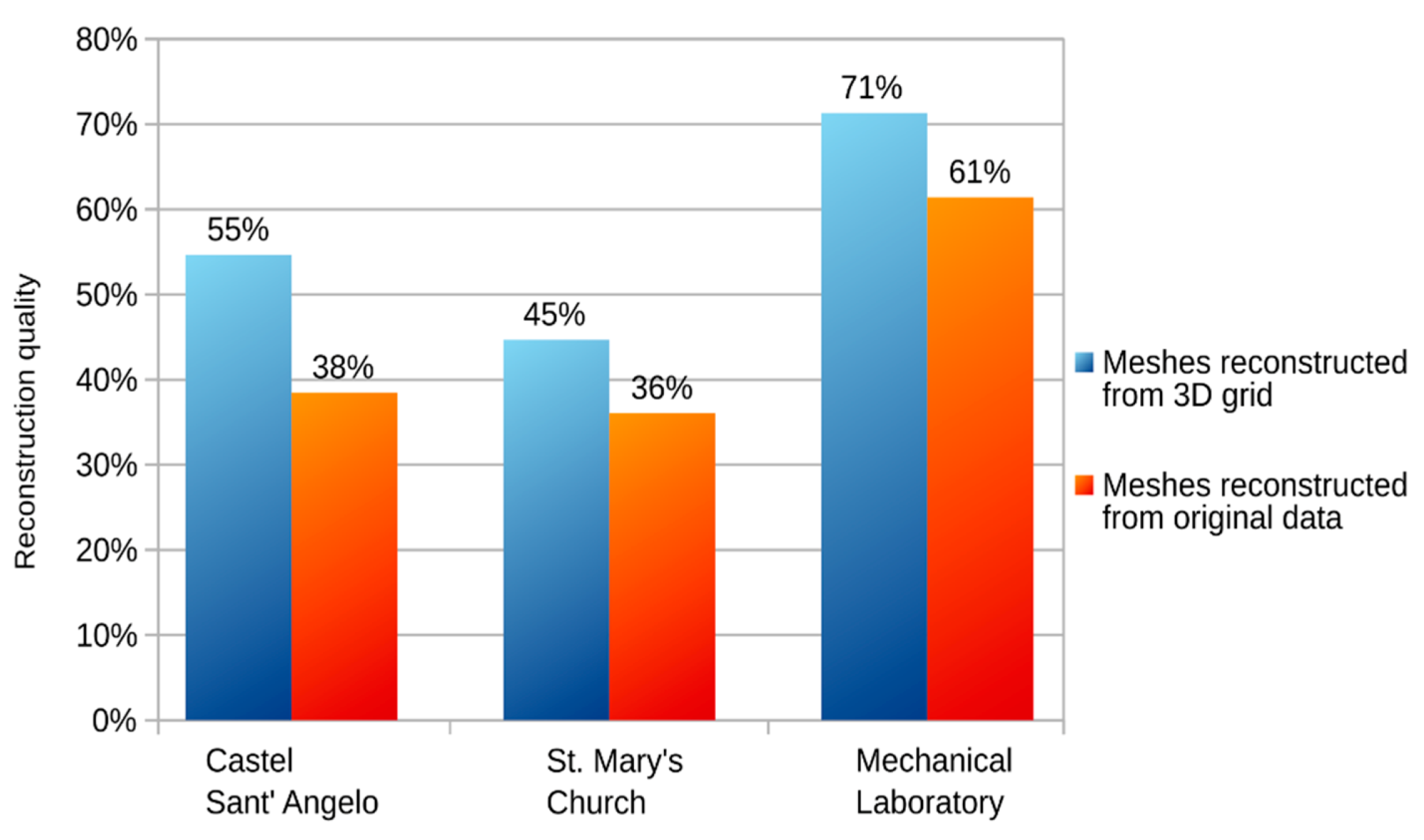
3.1. Determining Mesh Quality

For a primary, basic verification of a given object shape reconstruction method performance, visual evaluation by human is sufficient. However, for more objective and detailed verification, the ground truth models should be used along with the defined metrics. These metrics allow for automatic or semi-automatic comparison of a reconstructed model with a reference model and for the quantitative assessment of the degree of discrepancy between them.
Seitz et al. proposed the method for comparison of a 3D object model obtained by photogrammetry (the ground truth model—G) with a model derived from laser scanning data (the reconstructed model—R) [37]. The authors of the method introduce two quantities: accuracy and completeness. Based on calculating for each vertex in R the distance to the nearest vertex in G, the accuracy is defined as the percentage of vertices in R for which their distance to the nearest vertex in G is smaller than a given, defined threshold. The completeness evaluates quantitatively what part of G is actually contained in R.
The approach close to the mentioned above is used by the Metro tool [38] for evaluation of geometric differences between two 3D object models where one model is the simplification of another. This method does not operate only with vertices, but relies on random selecting the points on the R object surface for the distance calculation. This approach provides the user with additional information regarding the size of errors in tested areas, however, due to the random selection of test points, the results obtained with the use of Metro are non-deterministic.
Lavoué [39] proposed the method inspired by the approach used for 2D images quality comparison. In general, it relies on assessment of distortions around corresponding vertices in R and G, expressing the degree of the distortions by the specialized texture and then calculation of the overall degree of distortion.
It can be seen that many different approaches can be used for determining mesh quality. The qualitative metrics used in this work are primarily inspired by the previously described solution [37] based on comparing model pairs by calculating the distance between all of their individual vertices, which is a deterministic process that can be completed within a reasonably short amount of time and is guaranteed to always return identical results for the same object. The proposed metrics also extends the idea of comparing vertices by including vertex normals in the calculations. In detail, the proposed procedure for assessing the quality of a given reconstruction method is as follows: for each vertex of the ground truth model G, the corresponding nearest vertex in the reconstructed model R is searched (assuming that both models are placed in the same place in three-dimensional space), then the direct distance between these vertices and the value of the scalar product between their normal vectors are calculated. Then the following values are determined:
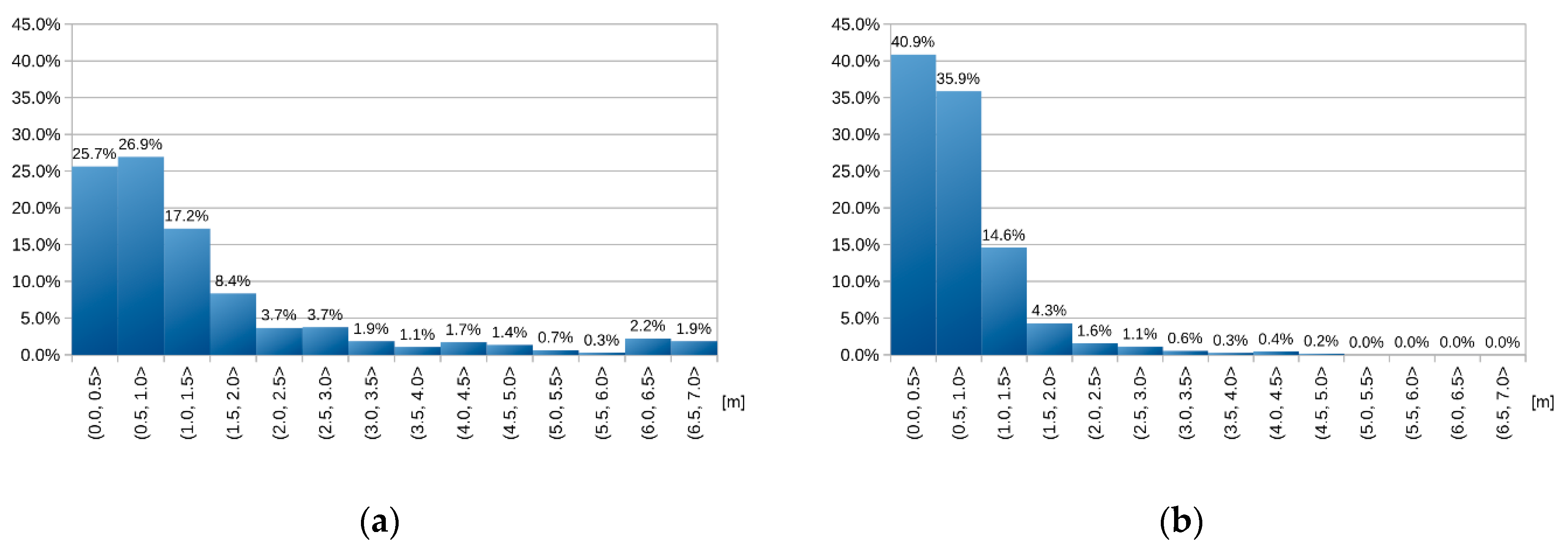
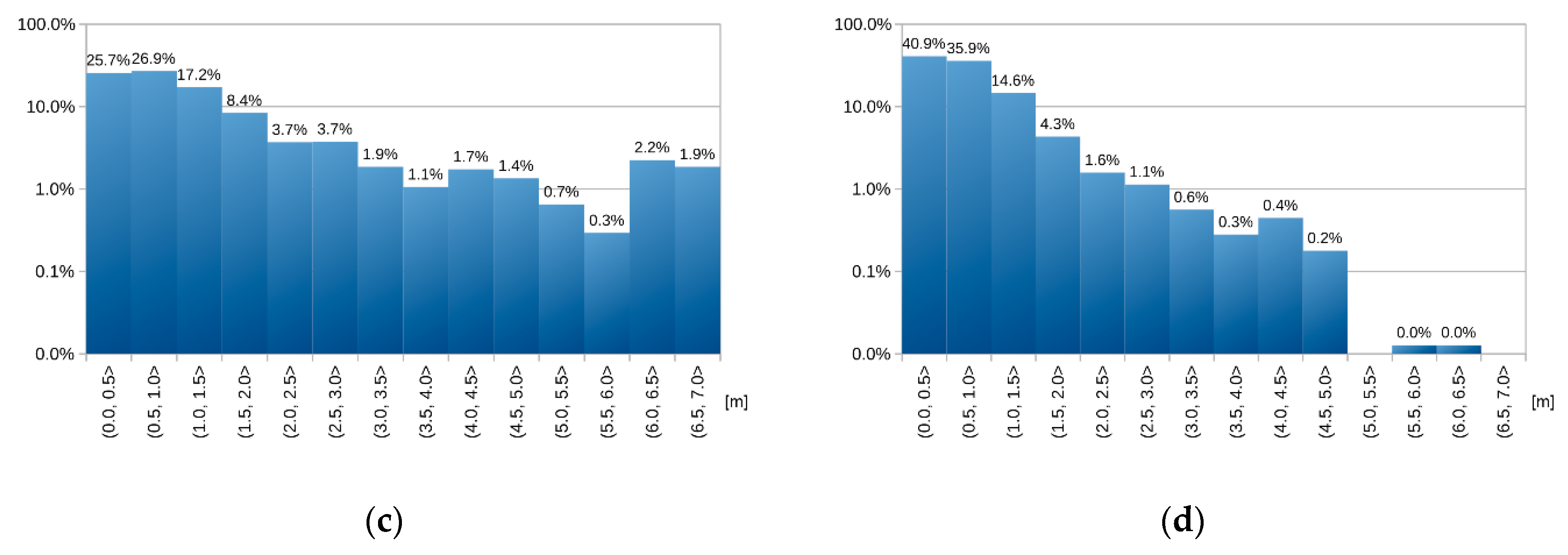
  • The smallest, average and largest distance between the vertices of model G and the nearest vertices of model R. Obviously, a perfectly reproduced model R should have the smallest possible values of these distances;
  • Vertex position accuracy (expressed as a percentage), being understood here as the number of vertices on G for which the distances to the corresponding vertices on R do not exceed a certain value (this value was experimentally established as one meter), divided by the number of all vertices on G. If R contains numerous distortions or “holes”, it should be expected that the calculated value will be low;
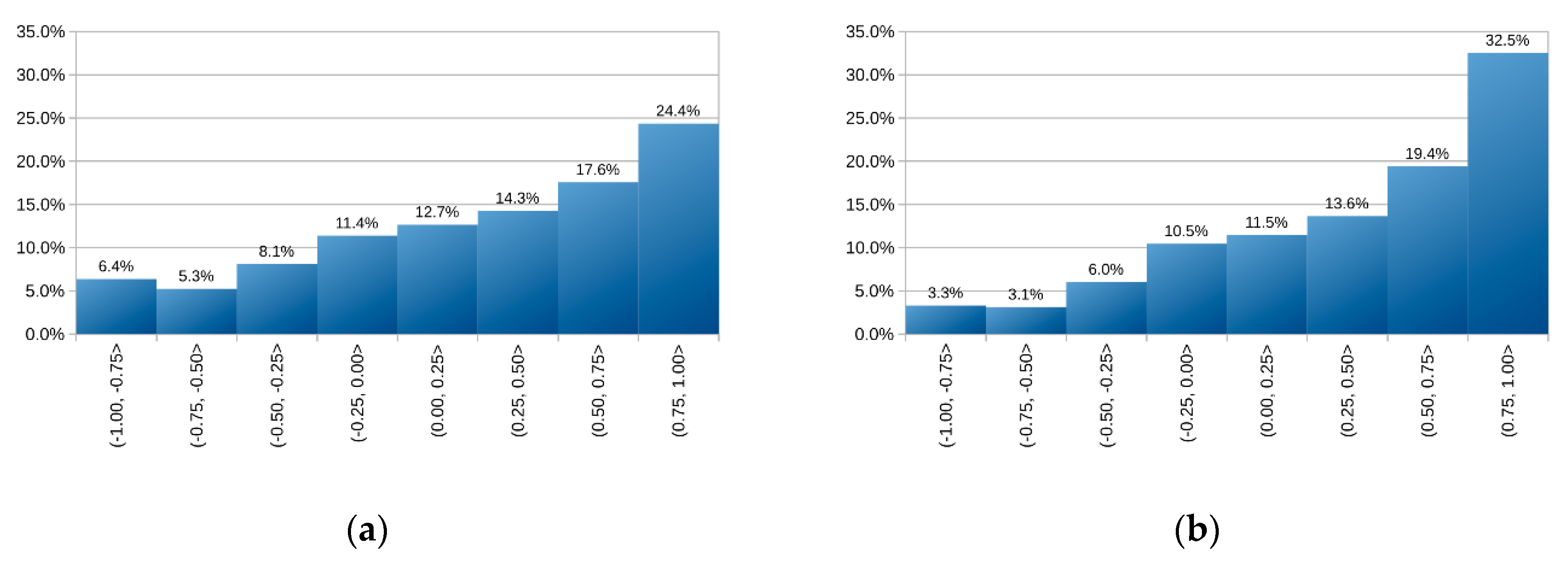
  • The smallest, average and largest differences between respective normal vectors of G and R, where this difference is defined as dot product of normal vectors of vertices. It is worth noting that dot product returns values in the range of <-1, 1> where -1 means that both vectors are parallel to each other, but they have opposite turns, 0 means that these vectors are perpendicular to each other and 1 means that both vectors have the same direction. Since the normal of a given vertex is by definition a unit vector, a dot product equal to 1 for normal vectors of two corresponding vertices would denote the perfect match;
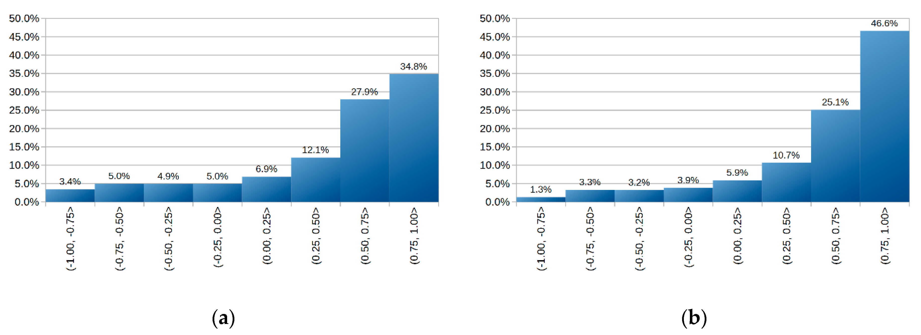
  • The accuracy of normal vectors (expressed as a percentage), understood here as the number of vertices in G for which the difference between respective normal vectors of G and R is not less than 0.75;
  • The number of resulting solids, i.e., how many independent meshes the reconstructed model consists of. In the tested cases, it was assumed that the ideal model of the tested object should consist of a single solid.
In addition, the calculated distances between individual vertices are divided into intervals, which are then visualized with histograms to better visualize the frequency of errors of specific range. The assumption of this action is that models generated by more accurate shape reconstruction methods could have a large number of small errors (distances close to zero) and a small number of large errors (distances in the range of several meters). The same approach was also used for the values of dot products between normal vectors in both models.

4. Results and Discussion

The following section presents the results of using data processing methods described in the previous chapter. Then both original and processed point cloud data were used as an input in the process of reconstructing three-dimensional meshes by using the Poisson surface reconstruction method implementation provided by MeshLab [40]. The output models are then compared in terms of their quality on the basis of the criteria discussed in Section 3.1 and the reference models presented in Section 2.2. As the Poisson surface reconstruction method has a tendency to randomly create a large amount of redundant surfaces around the base of the reconstructed objects, before comparing the results, all output meshes were properly preprocessed in order to remove any elements located below the lowest point of the original input data. This situation is illustrated in Figure 8 with the example of the results obtained for the Mechanical Laboratory building of the Faculty of Mechanics of the Gdansk University of Technology. Figure 8a,c present the direct results of performing surface reconstruction, while Figure 8b,d depict the trimmed versions of these meshes.
The following naming conventions were adopted: let us denote the ground truth model as G, the model reconstructed from the original data as R1 (Figure 8a,b) and the model reconstructed from 3D grid as R2 (Figure 8c,d). The presented results are the best ones obtained for each data set. The input parameters of the Poisson surface reconstruction method were identical for both processed and original data.
The first test case describes the shape of St. Mary’s Church in Gdansk, which is 104 m tall. Table 1 presents the input parameters of the 3D grid conversion algorithm, which were chosen empirically. The original point cloud consists of 69,142 points and was converted into a grid consisting of 41 height levels, thus creating a point set of 106,421 points. In particular, noteworthy here is the use of a high level of filling the empty elements between each level of the grid in order to complement the outer surfaces representing the side walls of the building and its main tower. In addition, thanks to the hybrid mode option, the processed point cloud contains all the details found in the original data, while thanks to the high level of the blur, the resulting model does not contain significant distortions on the roof surface.
Figure 9 presents: LiDAR scanning results limited to the area of St. Mary’s Church in Gdansk (a), the R1 mesh (c) generated on their basis, the same scanning results converted to 3D grid (b), the R2 mesh (d) created on their basis and the reference model G (e) with which the other meshes were compared. It can easily be seen that R1 has large gaps within the main tower, while R2 represents the entire object. A similar situation occurs in the case of the other turrets, which in R1 are represented by separate blocks placed loosely in space, while in R2 the same turrets are represented more accurately, although they are much lower than the actual towers visible both in G and the original point cloud.
Figure 10 shows the distance distributions between individual vertices of G and the corresponding vertices in reconstructed models. The values of these distances were grouped into ranges and the distributions were presented in the form of histograms to illustrate the frequency of different errors. Figure 10a shows the histogram of the distances between the vertices of G and R1, while Figure 10b shows the histogram of the distances between the vertices of G and R2. Additionally, Figure 10c,d depict the same results, but using a logarithmic scale on the distance axis. Each bar represents a certain range of distances, and its height indicates how much of the vertices of the entire model fall within their range in terms of their values. For example, in R1 20.8% of its vertices are located no more than half a meter from the position of the corresponding vertices in G, while in R2 the number of vertices not exceeding this distance is 22.2%. At the same time, in R2 you can see a smaller number of vertices whose distances from the vertices in G exceed five meters. Otherwise, the distance distributions of R1 and R2 are similar.
Figure 11 shows a comparison between reconstructed 3D models and the reference mesh in terms of the similarity between the normal vectors of their vertices. Figure 11a shows the distributions of the dot product of normal vectors for vertices of G and normal vectors of the corresponding vertices in R1, while Figure 11b shows identical comparison for meshes G and R2. It can be seen that the results for R2 are in this case much better than the results for R1: for R1, 34.8% of its normal vectors of vertices exceed the dot product value of 0.75, while in R2 this condition is fulfilled for 46.6% of its vertices. In the ideal case, the dot product of vector normals for corresponding vertices should be equal to 1.
Table 2 presents a summary of the most important criteria determining the quality of the R1 model (“reconstruction from original data”) and R2 model (“reconstruction from processed data”). Bold values mean better results in a given category. It can be seen that R2 obtained definitely better results than R1 in almost every category, especially in terms of the total number of resulting solids (ideally, the model should consist of a single mesh). The only category in which R2 is of inferior quality than R1 is the largest distance in the entire set that occurs between the vertices of G and the vertices of the reconstructed model. This case is illustrated in Figure 12, where in Figure 12a a single vertex of G is marked in red, for which the distance to the nearest vertex in R2 (Figure 12c) is the largest. For comparison, the corresponding vertex in R1 is shown in Figure 12b. It can be seen that these are the vertices corresponding to the towers of the Basilica, which in both cases were reproduced only to a small extent. In R1, a small body hovering over the rest of the model was treated as the top of the turret, while in R2 this turret is not present, therefore the closest part of the roof was considered its equivalent.
The second test case describes the surface scanning results for the Mechanical Laboratory building of the Faculty of Mechanics of the Gdansk University of Technology, 51 m tall, for which a detailed reference model was created based on its architectural plans. Table 3 presents the input parameters of the 3D grid conversion algorithm, which were chosen empirically. Since the original point cloud is characterized by high spatial resolution and consists of 89,485 points, small dimensions for a single sector were chosen and as a result the data were divided into 68 height levels. Similar to the previous test case, a high level of filling the empty elements between each level of the grid was used here, as well as a high level of the blur. In this case, however, the hybrid mode option was not used, because the original set of points was characterized by a large spatial irregularity, which would have a negative impact on the shape of the restored model. Since the generated point cloud was not merged with the original data set, the resulting point cloud consists of 84,882 points, which is less than the number of points contained in the original data.
Figure 13 presents: LiDAR scanning results limited to the area of the Mechanical Laboratory building (a) and the R1 model (c) generated on their basis, the same results converted to 3D grid (b) and the R2 (d) model created on their basis, as well as the reference model G (e). Figure 13 also includes close-ups of the tower roof, so it can be seen that in R1 the tower model contains distortions below its roof and within the chimney, which are not present in R2. At the same time, R1 contains a large number of redundant surfaces in the lower parts of the object which are not present in either R2 or the reference model G.
Figure 14 shows the distance distributions between individual vertices of G and the corresponding vertices in reconstructed models, grouped in the same way as before. Figure 14a shows the histogram of the distances between the vertices of G and R1, while Figure 14b shows the histogram of the distances between the vertices of G and R2 Additionally, Figure 14c,d depict the same results, but using a logarithmic scale on the distance axis. For both reconstructed models, it can be seen that about half of their vertices are in close proximity (max. 40 cm) to the corresponding vertices in G and the number of errors significantly decreases with the increase of interval values. It is worth noting that in R2 there is definitely a smaller number of vertices whose distance from the corresponding points in G exceeds 120 cm. This means that in this case, the use of the 3D grid conversion algorithm results in the creation of a model with a small number of large errors, at the expense of a minor increase in the number of small errors.
Figure 15 shows a comparison between reconstructed 3D models and the reference mesh in terms of the similarity between the normal vectors of their vertices. Figure 15a shows the distributions of the dot product of normal vectors for vertices of G and normal vectors of the corresponding vertices in R1, while Figure 15b shows the identical comparison for meshes G and R2. While in general both histograms are quite similar to each other, it is worth to note that R2 achieves in this case much better results than R1, since for R1 42.2% of all its vertices exceed the dot product value of 0.75, while in R2 the number of such vertices is at 51.2%. In addition, R2 contains smaller number of vertices for which the calculated dot product is negative.
Table 4 presents a summary of the most important criteria determining the quality of the R1 model (“reconstruction from original data”) and R2 model (“reconstruction from processed data”). It can be seen that R2 once again obtained better results than R1 in almost every category, however it does have a worse result for the minimum distance between its vertices and the corresponding vertices of G. Nevertheless, the result obtained for R2 is worse by only 4 mm.
The last test case consists of simulated surface scanning results obtained for a mesh of Castel Sant’Angelo, containing 11,105 points. Table 5 presents the input parameters of the 3D grid conversion algorithm, which are almost identical to those used for St. Mary’s Church in Gdansk, however, for this case, smaller sector dimensions were adopted due to the denser distribution of points on the Z axis. The input point cloud, which was obtained from a mesh of a 37 m tall object, was divided into 38 levels, creating a data set of 72,669 points.
Figure 16 shows the results of the simulated scanning (a) and the R1 model (b) generated on their basis, the same results converted to 3D grid (c) and the R2 model (d) created on their basis, as well as the reference model G (e), which in this case also serves as the input model for the scanning simulation process. It can be seen that the R2 model more accurately reflects the shape of the vertical surfaces.
Figure 17 shows the distance distributions between individual vertices of G and the corresponding vertices in reconstructed models. Figure 17a shows the histogram of the distances between the vertices of G and R1, while Figure 17b shows the histogram of the distances between the vertices of G and R2. Additionally, Figure 17c,d depict the same results, but using a logarithmic scale on the distance axis. In this case, the R2 model exceeds R1 in almost every aspect. It is particularly worth noting that in R2 91.4% of its vertices are no more than 1.5 m from the corresponding vertices in G, while in R1 only 69.8% of its vertices meet this criterion. In addition, in R2 only a small number of its vertices are located more than 5 m from their counterparts in G.
Figure 18 shows a comparison between reconstructed 3D models and the reference mesh in terms of the similarity between the normal vectors of their vertices. Figure 18a shows the distributions of the dot product of normal vectors for vertices of G and normal vectors of the corresponding vertices in R1, while Figure 18b shows identical comparison for meshes G and R2. In this case, the results obtained for R2 are generally better than the results obtained for R1, especially in the range of (0.75, 1.0].
Table 6 presents a summary of the most important criteria determining the quality of the R1 model (“reconstruction from original data”) and R2 model (“reconstruction from processed data”). This time, R2 exceeds R1 in all categories. The greatest advantage of R2 over R1 is visible in the case of the average distance between its vertices and the vertices of model G, where the result obtained for R2 is about 50 times better than R1.
To sum up, for the presented cases the overall quality of models reconstructed from 3D grids is definitely higher than in the case of meshes reconstructed from original point clouds. By introducing an additional value for the quality of the reconstruction, defined as an arithmetic average of the values of the accuracy of the vertex positions at the threshold of one meter and the normal vectors accuracy at the threshold of 0.75, then a summary of the quality results of individual models could be expressed using Figure 19.

5. Conclusions

The study presents a novel method of point cloud data processing for the purpose of 3D shape reconstruction. The performance and quality of the proposed algorithm was tested using real-world data and compared against high quality reference data. In its current state, the proposed algorithm is not meant to be used as a standalone tool. Instead, its purpose is to perform additional preprocessing before applying existing surface reconstruction methods, which allows for the generation of more detailed 3D meshes. The algorithm was shown to positively influence the quality of 3D models reconstructed from the processed datasets. In specific, application of the proposed algorithm allowed to decrease the average distance between the vertices of the reconstructed model and the ground truth model by no less than 20% in all presented cases.
Further improvements in the approach will concentrate on better tuning the reconstruction procedure to specific features of different reconstructed shapes and, on the other hand, on automatic selection of the optimal control parameter values needed by the algorithm. The latter may be achieved by using some catalog of rules suggesting the values of parameters to be chosen and tested in several cases or by applying the machine learning techniques alternatively. At the end, it may be noticed that currently, due to the lack of better options, various companies and institutions working with three-dimensional visualization of terrestrial environments are often limited to the use of primitive methods of shape reconstruction based on height maps and hand-made simplified models of individual objects. Only few entities can afford to obtain spatial data that has enough information to be able to automatically generate detailed models of satisfactory quality on their basis. The input data processing methods proposed in this work have the potential to automatically reproduce models with a similar level of complexity based on lower quality data. What is more, the presented methods are not limited to specific data sources and can be applied to virtually any kind of point cloud data. In the future, they can serve as inspiration to create even better-quality solutions based on similar processing methods.

Author Contributions

All authors contributed as below: “Conceptualization, M.K.; methodology, M.K.; software, M.K.; validation, M.K. and Z.L.; formal analysis, Z.L.; investigation, M.K. and Z.L.; resources, M.K. and Z.L.; writing—original draft preparation, M.K.; writing—review and editing, Z.L.; visualization, M.K.; supervision, Z.L.;. All authors have read and agreed to the published version of the manuscript.

Funding

This research received no external funding.

Acknowledgments

The authors would like to thank the Polish Centre of Geodesic and Cartographic Documentation for providing them with LiDAR data.

Conflicts of Interest

The authors declare no conflict of interest.

References

  1. Kulawiak, M.; Łubniewski, Z.; Bikonis, K.; Stepnowski, A. Geographical Information System for analysis of Critical Infrastructures and their hazards due to terrorism, man-originated catastrophes and natural disasters for the city of Gdansk. In Lecture Notes in Geoinformation and Cartography; Springer: Berlin/Heidelberg, Germany, 2009; pp. 251–262. [Google Scholar] [CrossRef]
  2. Drypczewski, K.; Moszyński, M.; Demkowicz, J.; Bikonis, K.; Stepnowski, A. Design of the Dual Constellation Gps/Galileo Mobile Device for Improving Navigation of the Visually Impaired in an Urban Area. Pol. Marit. Res. 2015, 22, 15–20. [Google Scholar] [CrossRef] [Green Version]
  3. Manferdini, A.M.; Russo, M. Multi-scalar 3D digitization of Cultural Heritage using a low-cost integrated approach. In Proceedings of the 2013 Digital Heritage International Congress (DigitalHeritage), Marseille, France, 28 October–1 November 2013; pp. 153–160. [Google Scholar]
  4. Pavlidis, G.; Koutsoudis, A.; Arnaoutoglou, F.; Tsioukas, V.; Chamzas, C. Methods for 3D digitization of Cultural Heritage. J. Cult. Herit. 2007, 8, 93–98. [Google Scholar] [CrossRef] [Green Version]
  5. Dąbrowski, J.; Kulawiak, M.; Moszyński, M.; Bruniecki, K.; Kamiński, Ł.; Chybicki, A.; Stepnowski, A. Real-time web-based GIS for analysis, visualization and integration of marine environment data. In Information Fusion and Geographic Information Systems; Springer: Berlin/Heidelberg, Germany, 2009; pp. 277–288. [Google Scholar] [CrossRef]
  6. Kulawiak, M.; Bikonis, K.; Stepnowski, A. Dedicated geographical information system in the context of critical infrastructure protection. In Proceedings of the 1st International Conference on Information Technology, Gdańsk, Poland, 19–21 May 2008; pp. 157–162. [Google Scholar]
  7. Rossetti, M.D.; Trzcinski, G.F.; Syverud, S.A. Emergency department simulation and determination of optimal attending physician staffing schedules. In Proceedings of the WSC’99. 1999 Winter Simulation Conference Proceedings. ‘Simulation - A Bridge to the Future’ (Cat. No.99CH37038), Phoenix, AZ, USA, 5–8 December 1999; Volume 2, pp. 1532–1540. [Google Scholar]
  8. Wang, Z.; Schenk, T. Building extraction and reconstruction from lidar data. Int. Arch. Photogramm. Remote Sens. 2000, 33(part B3), 958–964. [Google Scholar]
  9. Rost, H.; Grierson, H. High Precision Projects using LiDAR and Digitial Imagery. In Proceedings of the TS11-Imaging and Data Applications, Integrating Generations, FIG Working Week, Stockholm, Sweden, 14–19 June 2008. [Google Scholar]
  10. Nikic, D.; Wu, J.; Pauca, P.; Plemmons, R.; Zhang, Q. A novel approach to environment reconstruction in lidar and hsi datasets. In Proceedings of the Advanced Maui Optical and Space Surveillance Technologies Conference, Maui, HI, USA, 11–14 September 2012; Volume 1, p. 81. [Google Scholar]
  11. Huber, M.; Schickler, W.; Hinz, S.; Baumgartner, A. Fusion of LIDAR data and aerial imagery for automatic reconstruction of building surfaces. Proceedings of 2003 2nd GRSS/ISPRS Joint Workshop on Remote Sensing and Data Fusion over Urban Areas, Berlin, Germany, 22–23.May.2003; pp. 82–86. [Google Scholar]
  12. Dharmapuri, S.; Tully, M. Evolution of Point Cloud. LIDAR Mag. 2018. Available online: https://lidarmag.com/2018/07/16/evolution-of-point-cloud/ (accessed on 28 November 2018).
  13. Floriani, L.D.; Magillo, P. Triangulated Irregular Network. In Encyclopedia of Database Systems; Springer: Boston, MA, USA, 2009; pp. 3178–3179. [Google Scholar] [CrossRef]
  14. Kazhdan, M.; Bolitho, M.; Hoppe, H. Poisson Surface Reconstruction. In Proceedings of the 4th Eurographics Symposium on Geometry Processing, Cagliari, Italy, 26–28 June 2006; pp. 61–70. [Google Scholar]
  15. Kada, M.; McKinley, L. 3D building reconstruction from LiDAR based on a cell decomposition approach. Int. Arch. Photogramm. Remote Sens. Spat. Inf. Sci 2009, 38, 47–52. [Google Scholar]
  16. Kim, K.; Shan, J. Building roof modeling from airborne laser scanning data based on level set approach. Isprs J. Photogramm. Remote Sens. 2001, 66, 484–497. [Google Scholar] [CrossRef]
  17. Henn, A.; Gröger, G.; Stroh, V.; Plümer, L. Model driven reconstruction of roofs from sparse LIDAR point clouds. Isprs J. Photogramm. Remote Sens. 2013, 76, 17–29. [Google Scholar] [CrossRef]
  18. Cheng, L.; Tong, L.; Chen, Y.; Zhang, W.; Shan, J.; Liu, Y.; Li, M. Integration of LiDAR data and optical multi-view images for 3D reconstruction of building roofs. Opt. Lasers Eng. 2013, 51, 493–502. [Google Scholar] [CrossRef]
  19. Babahajiani, P.; Fan, L.; Kämäräinen, J.K.; Gabbouj, M. Urban 3D segmentation and modelling from street view images and LiDAR point clouds. Mach. Vis. Appl. 2017, 679–694. [Google Scholar] [CrossRef]
  20. Yi, C.; Zhang, Y.; Wu, Q.; Xu, Y.; Remil, O.; Wei, M.; Wang, J. Urban building reconstruction from raw LiDAR point data. Comput.-Aided Des. 2017, 1–14. [Google Scholar] [CrossRef]
  21. Chen, D.; Wang, R.; Peethambaran, J. Topologically aware building rooftop reconstruction from airborne laser scanning point clouds. IEEE Trans. Geosci. Remote Sens. 2017, 7032–7052. [Google Scholar] [CrossRef]
  22. Bauchet, J.P.; Lafarge, F. City reconstruction from airborne LiDAR: A computational geometry approach. 2019. Available online: https://easychair.org/publications/preprint/pLtR (accessed on 4 May 2020).
  23. Wang, R.; Peethambaran, J.; Dong, C. LiDAR Point Clouds to 3D Urban Models: A Review. IEEE J. Sel. Top. Appl. Earth Obs. Remote Sens. 2018, 11. Available online: https://www.researchgate.net/publication/321500340_LiDAR_Point_Clouds_to_3D_Urban_Models_A_Review (accessed on 4 May 2020). [CrossRef]
  24. Kazhdan, M.; Hoppe, H. Screened Poisson Surface Reconstruction. Acm Trans. Graph. 2013, 32. [Google Scholar] [CrossRef] [Green Version]
  25. Bernardini, F.; Mittleman, J.; Ftushmeier, H.; Silva, C.; Taubin, G. The Ball-Pivoting Algorithm for Surface Reconstruction. IEEE Trans. Vis. Comput. Graph. 1999, 5, 349–359. [Google Scholar] [CrossRef]
  26. Tsai, V.J.D. Delaunay triangulations in TIN creation: An overview and a linear-time algorithm. Int. J. Geogr. Inf. Syst. 1993, 7, 501–524. [Google Scholar] [CrossRef]
  27. Amenta, N.; Choi, S.; Kolluri, R.K. The Power Crust. In Proceedings of the Sixth ACM Symposium on Solid Modeling and Applications, Ann Arbor, MI, USA, 6–8 June 2001; pp. 249–266. [Google Scholar]
  28. Kulawiak, M.; Łubniewski, Z. 3D Object Shape Reconstruction from Underwater Multibeam Data and Over Ground Lidar Scanning. Pol. Marit. Res. 2018, 25, 47–56. [Google Scholar] [CrossRef] [Green Version]
  29. Zhang, L.; Zhang, L. Deep learning-based classification and reconstruction of residential scenes from large-scale point clouds. IEEE Trans. Geosci. Remote Sens. 2017, 1887–1897. [Google Scholar] [CrossRef]
  30. Tse, R.O.C.; Gold, C.M.; Kidner, D.B. Building reconstruction using LIDAR data. In Proceedings of the 4th ISPRS Workshop on Dynamic and Multi-dimensional GIS, Pontypridd, Wales, UK, 5–8 September 2005; pp. 156–161. [Google Scholar]
  31. Kulawiak, M.; Łubniewski, Z. Reconstruction Methods for 3D Underwater Objects Using Point Cloud Data. Hydroacoustics 2015, 18, 95–102. [Google Scholar]
  32. Polish Head Office of Geodesy and Cartography (GUGIK). Numerical elevation models. Available online: https://www.geoportal.gov.pl/en/dane/numeryczne-modele-wysokosciowe (accessed on 30 March 2020).
  33. blender.org - Home of the Blender project - Free and Open 3D Creation Software. Available online: https://www.blender.org/ (accessed on 30 March 2020).
  34. Kulawiak, M. Programmatic Simulation of Laser Scanning Products. In Proceedings of the IEEE SPA 2018 Signal Processing Algorithms, Architectures, Arrangements, and Applications, Poznań, Poland, 9–21 September 2018. [Google Scholar]
  35. OGRE - Open Source 3D Graphics Engine. Available online: https://www.ogre3d.org (accessed on 6 May 2020).
  36. CSA. Castelo De Santo Angelo (Castel Sant’Angelo). 3D Warehouse. Available online: https://3dwarehouse.sketchup.com/model/e6b5d74421f6aaf3ee1dec833bfa8b3/Castelo-De-Santo-Angelo-Castel-SantAngelo (accessed on 11 July 2018).
  37. Seitz, S.M.; Curless, B.; Diebel, J.; Scharstein, D.; Szeliski, R. A Comparison and Evaluation of Multi-View Stereo Reconstruction Algorithms. In Proceedings of the IEEE Computer Society Conference on Computer Vision and Pattern Recognition, New York, NY, USA, 17–22 June 2006; 2006; pp. 519–528. [Google Scholar]
  38. Cignoni, P.; Rocchini, C.; Scopigno, R. Metro: Measuring Error on Simplified Surfaces; Centre National de la Recherche Scientifique: Paris, France, 1996. [Google Scholar] [CrossRef] [Green Version]
  39. Lavoué, G. A Multiscale Metric for 3D Mesh Visual Quality Assessment. Comput Graph. Forum 2011, 30, 1427–1437. [Google Scholar] [CrossRef]
  40. Cignoni, P.; Callieri, M.; Corsini, M.; Dellepiane, M.; Ganovelli, F.; Ranzuglia, G. MeshLab: An Open-Source Mesh Processing Tool. In Proceedings of the Eurographics Italian Chapter Conference, Salerno, Italy, 2–4 July 2008. [Google Scholar]
Figure 1. Objects scanned via airborne light detection and ranging (LiDAR) from a high altitude exhibit missing data on surfaces parallel to the laser beam.
Remotesensing 12 01643 g001
Figure 2. Reference model of St. Mary’s Church in Gdansk acquired with the use of photogrammetry.
Remotesensing 12 01643 g002
Figure 3. Reference model of the Mechanical Laboratory building of the Faculty of Mechanics of the Gdansk University of Technology made by hand based on its architectural plans.
Remotesensing 12 01643 g003
Figure 4. Conversion of the point cloud representing the result of (a) scanning the surface of St. Mary’s Church in Gdansk into (b) a simplified 3D mesh consisting of (c) four raster layers, where the pixel value represents its location on the vertical axis within a given layer.
Remotesensing 12 01643 g004
Figure 5. 3D grid conversion and surface reconstruction process.
Remotesensing 12 01643 g005
Figure 6. Comparison of the original point cloud derived from the results of (a) scanning the surface of St. Mary’s Church in Gdansk with (b) the point cloud converted to 3D grid.
Remotesensing 12 01643 g006
Figure 7. Results of (c,f) the screened Poisson surface reconstruction method compared to the results obtained by (b,e) regular Poisson surface reconstruction method for (a) original point cloud and (d) obtained 3D grid for data representing Castel Sant’Angelo.
Remotesensing 12 01643 g007aRemotesensing 12 01643 g007b
Figure 8. Result models representing the Mechanical Laboratory building of the Faculty of Mechanics of the Gdansk University of Technology (a) obtained from original data and (c) 3D grid and (b,d) their trimmed versions.
Remotesensing 12 01643 g008
Figure 9. Data showing the meshes of St. Mary’s Church in Gdansk. (a) LiDAR scanning results and (c) the model generated on their basis, (b) 3D grid and (d) the model created on its basis, as well as (e) the reference model.
Remotesensing 12 01643 g009
Figure 10. Distance distributions (a) between the vertices of G and R1, as well as (b) between the vertices of G and R2 regarding meshes depicting St. Mary’s Church in Gdansk. Histograms (c) and (d) show the same results using a logarithmic scale.
Remotesensing 12 01643 g010
Figure 11. Histograms of dot product values of normal vectors of (a) vertices of G and R1 and (b) vertices of G and R2, regarding meshes depicting St. Mary’s Church in Gdansk.
Remotesensing 12 01643 g011
Figure 12. Vertex representing the top of one of the turrets of (a) the reference model of St. Mary’s Church in Gdansk and the corresponding vertices in the (b) R1 and (c) R2 models.
Remotesensing 12 01643 g012
Figure 13. Data showing the meshes of the Mechanical Laboratory building. (a) LiDAR scanning results and (c) the model generated on their basis, (b) 3D grid and (d) the model created on its basis, as well as (e) the reference model.
Remotesensing 12 01643 g013
Figure 14. Distance distributions between (a) the vertices of G and R1, as well as between (b) the vertices of G and R2 regarding meshes depicting the Mechanical Laboratory building. Histograms (c) and (d) show the same results using a logarithmic scale.
Remotesensing 12 01643 g014
Figure 15. Histograms of (a) dot product values of normal vectors of vertices of G and R1 and (b) vertices of G and R2 regarding meshes depicting the Mechanical Laboratory building.
Remotesensing 12 01643 g015
Figure 16. Data showing the meshes of Castel Sant’Angelo. (a) LiDAR scanning results and (c) the model generated on their basis, (b) 3D grid and (d) the model created on its basis, as well as (e) the reference model.
Remotesensing 12 01643 g016
Figure 17. Distance distributions (a) between the vertices of G and R1, as well as (b) between the vertices of G and R2 regarding meshes depicting Castel Sant’Angelo. Histograms (c) and (d) show the same results using a logarithmic scale.
Remotesensing 12 01643 g017aRemotesensing 12 01643 g017b
Figure 18. Histograms of dot product values of normal vectors of (a) vertices of G and R1 and (b) vertices of G and R2, regarding meshes depicting Castel Sant’Angelo.
Remotesensing 12 01643 g018
Figure 19. Impact of using the cube algorithm for individual data sets on the quality of models reconstructed using the Poisson surface reconstruction method.
Remotesensing 12 01643 g019
Table 1. Input parameters of the algorithm used to convert point cloud data representing St. Mary’s Church in Gdansk into a 3D grid.
Dimensions of a Single Sector (XYZ) [m]0.5 × 0.5 × 2.0
Option to fill empty elements within a single grid levelYES
Filtration intensity2
The level of filling the empty elements between each level of the grid20
Hybrid modeYES
Table 2. Comparison of results in the scope of quality criteria of individual models of St. Mary’s Church in Gdansk, reconstructed from original and processed data.
CriteriaReconstruction from Original Data (R1)Reconstruction from Processed Data (R2)
Minimum distance [cm]1.241.00
Average distance [cm]259.84189.83
Maximum distance [m]20.8127.66
Vertex position accuracy at the threshold of one meter37.29%42.78%
The average difference between respective normal vectors0.450.57
Normal vectors accuracy at the threshold of 0.7534.82%46.62%
The number of resulting solids3713
Table 3. Input parameters of the algorithm used to convert point cloud data representing the Mechanical Laboratory building.
Dimensions of a Single Sector (XYZ) [m]0.25 × 0.25 × 0.75
Option to fill empty elements within a single grid levelYES
Filtration intensity2
The level of filling the empty elements between each level of the grid10
Hybrid modeNO
Table 4. Comparison of results in the scope of quality criteria of individual models of the Mechanical Laboratory building, reconstructed from original and processed data.
CriteriaReconstruction from Original Data (R1)Reconstruction from Processed Data (R2)
Minimum distance [cm]0.250.65
Average distance [cm]63.3149.97
Maximum distance [m]6.442.47
Vertex position accuracy at the threshold of one meter80.64%91.48%
The average difference between respective normal vectors0.390.54
Normal vectors accuracy at the threshold of 0.7542.20%51.17%
The number of resulting solids3818
Table 5. Input parameters of the algorithm used to convert point cloud data representing Castel Sant’Angelo.
Dimensions of a Single Sector (XYZ) [m]0.5 × 0.5 × 1.0
Option to fill empty elements within a single grid levelYES
Filtration intensity2
The level of filling the empty elements between each level of the grid20
Hybrid modeYES
Table 6. Comparison of results in the scope of quality criteria of individual models of Castel Sant’Angelo, reconstructed from original and processed data.
CriteriaReconstruction from Original Data (R1)Reconstruction from Processed Data (R2)
Minimum distance (cm)4.030.78
Average distance (cm)165.853.31
Maximum distance (m)12.6811.72
Vertex position accuracy at the threshold of one meter52.60%76.77%
The average difference between respective normal vectors0.270.40
Normal vectors accuracy at the threshold of 0.7524.37%32.54%
Number of resulting solids43

