Article

Spatiotemporal Characterization of Land Cover Impacts on Urban Warming: A Spatial Autocorrelation Approach

Department of Geography, University of Idaho, Moscow, ID 83844, USA
*
Author to whom correspondence should be addressed.
Remote Sens. 2020, 12(10), 1631; https://doi.org/10.3390/rs12101631
Submission received: 14 April 2020 / Revised: 16 May 2020 / Accepted: 17 May 2020 / Published: 20 May 2020
(This article belongs to the Section Urban Remote Sensing)

Abstract

:
There has been an increasing concern of rising temperatures as cities continue to expand and intensify. Urban warming is having significant impacts on the environment that are far beyond city limits. Understanding the development pattern of the urban heat island (UHI) effect is crucial for making action plans to mitigate urban warming. In this study, we combine multitemporal satellite imagery, spatial autocorrelation indices, and statistical analysis into a spatiotemporal study of the surface UHI effect in the Boise-Meridian metropolitan area. A continuous landscape modeling perspective was taken to quantitatively depict the abundance and spatial configuration of green vegetation and built-up areas at a landscape scale. We aim to (1) evaluate the variations in the land surface temperatures (LST) along the urban–rural gradients of Boise for multiple years, (2) identify the relationships of the LST variations with the land cover variables quantified using the spatial autocorrelation indices, and (3) analyze the changing climate in Boise in conjunction with its urbanization pattern over the last two decades. Results show that the region experienced a significant increase in the LST along with a great expansion of urban areas at the cost of agriculture. The warming effect of built-up areas was greater than the cooling effect of green vegetation, suggesting an urgent need for increasing greenspace in the city. Statistical analyses show that clustered vegetation and dispersed built-up features are beneficial for reducing the LST. Our study presents a spatiotemporal framework for analyzing the surface UHI effect from multiple angles. Scientific findings from this study can help make informed policies against urban warming via optimal planning of urban land cover.

Graphical Abstract

1. Introduction

The world population is growing continuously with a projected population of 9.8 billion in 2050. The replacement of natural landscapes with human-induced features greatly alters the surface energy balance of a city, causing increased temperatures in urban areas in comparison to its rural surroundings, commonly referred to as the urban heat island (UHI) effect. The UHI effect can potentially increase a city’s water and energy consumption, lower its air and water quality, and more importantly, compromise human comfort and health [1]. There is a wide spectrum of heat-related health problems that are either triggered or exacerbated by increased daytime temperatures and reduced nighttime cooling. This puts sensitive population such as the elderly and children at particular risk. According to the Centers for Disease Control and Prevention, from 1979 to 2003, excessive heat events have caused more than 8000 premature deaths in the US. This exceeds the total mortality from many natural disasters combined [1].
A growing number of literature has focused on the UHI, in particular the land surface temperature (LST), in relation to the land cover characteristics [2,3,4,5]. The cooling effect from green vegetation is widely recognized while impervious surfaces including roads, parking lots, and pavements tend to increase the LST in cities [4,5,6,7]. More recent literature has focused on the relationships between the spatial configuration of land cover patches and LST [8,9,10]. They found that not only the proportion of land cover features affects the LST, their shape, size, diversity, and spatial arrangement also play an important role [11,12,13,14].
There is a heavy reliance on the landscape metrics to characterize the land composition and spatial configuration of land cover patches [8,13,15,16]. Despite a wide adoption of landscape metrics in a variety of fields, there are some caveats associated with the use of landscape metrics in UHI studies [17,18]. Since landscape metrics follow a patch-mosaic paradigm, the input to the program is a discrete land use land cover (LULC) map that is prepared beforehand. The variations in the spectral signatures within the discrete LULC classes are largely overlooked [12]. Further, the errors and uncertainties created in the categorization process not only exist in the classified LULC map but likely propagate into the results of the landscape pattern analysis [19]. An alternative route is to take on the continuous landscape modeling perspective. The continuous landscape modeling approach focuses on the combination of satellite image-derived biophysical variables and local indicators of spatial association [17,20]. This approach permits the assessment of feature abundance and spatial configuration at a local scale while preserving as many spatial details as possible in the original spectral signatures [17]. Moreover, it is capable of depicting gradual landscape changes at a per-pixel level [19]. Current literature shows great potential of using the continuous models in vegetation mapping [21], forest modeling [20], and analysis of urban landscape dynamics [19].
Thermal remote sensing provides long-term and repeated monitoring of the Earth’s surface with global spatial coverage and varying degrees of spatial details. It provides a useful tool for studying long-term LST changes. Cross-sectional evaluations of the LST focus on a single snapshot of the LST in time. Since the LST varies both spatially and temporally, a multidirectional and multitemporal approach can offer a better understanding of the LST patterns in the context of rapid urbanization and population explosion.
This paper presents a spatiotemporal UHI study utilizing multitemporal Landsat images, local indicators of spatial association, and urban–rural gradient analysis. Our research objectives are to (1) evaluate the spatiotemporal variations in the LST along the urban–rural gradients of the Boise-Meridian metropolitan area from 2001 to 2013, (2) identify the relationships of the LST variations with the changing land cover patterns represented using the spatial indicators, and (3) determine the linkage between the changing climate in Boise and its urbanization pattern in search of proper adaptation and mitigation strategies.

2. Materials and Methods
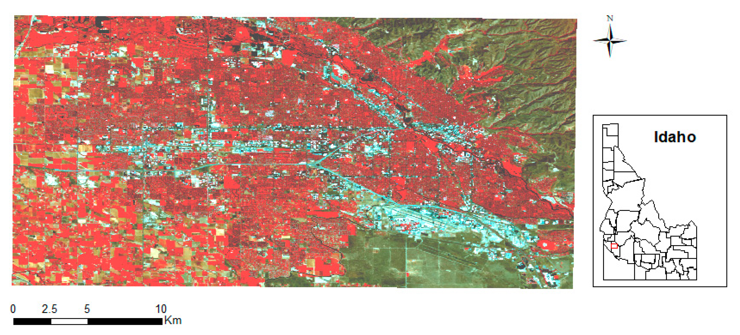
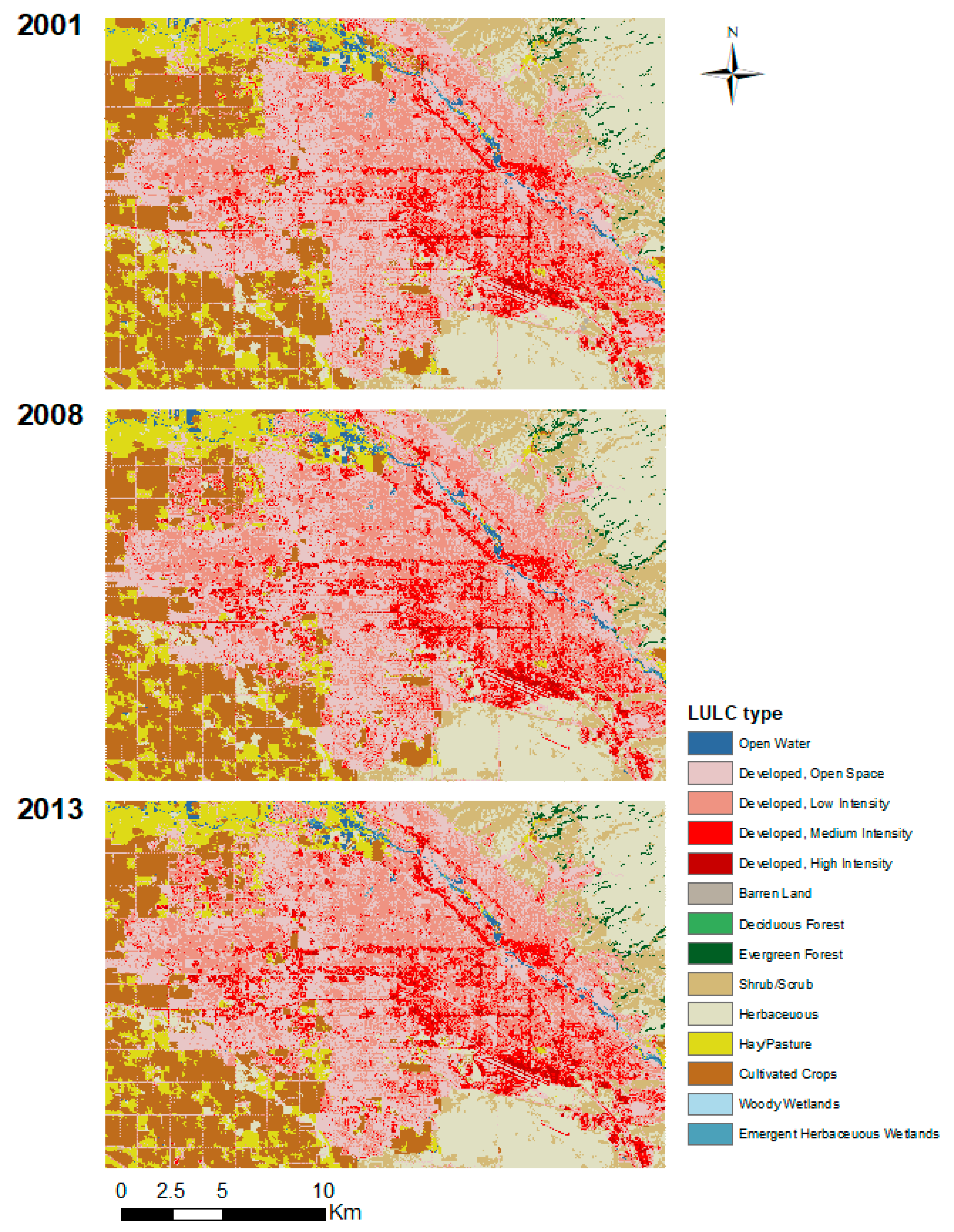
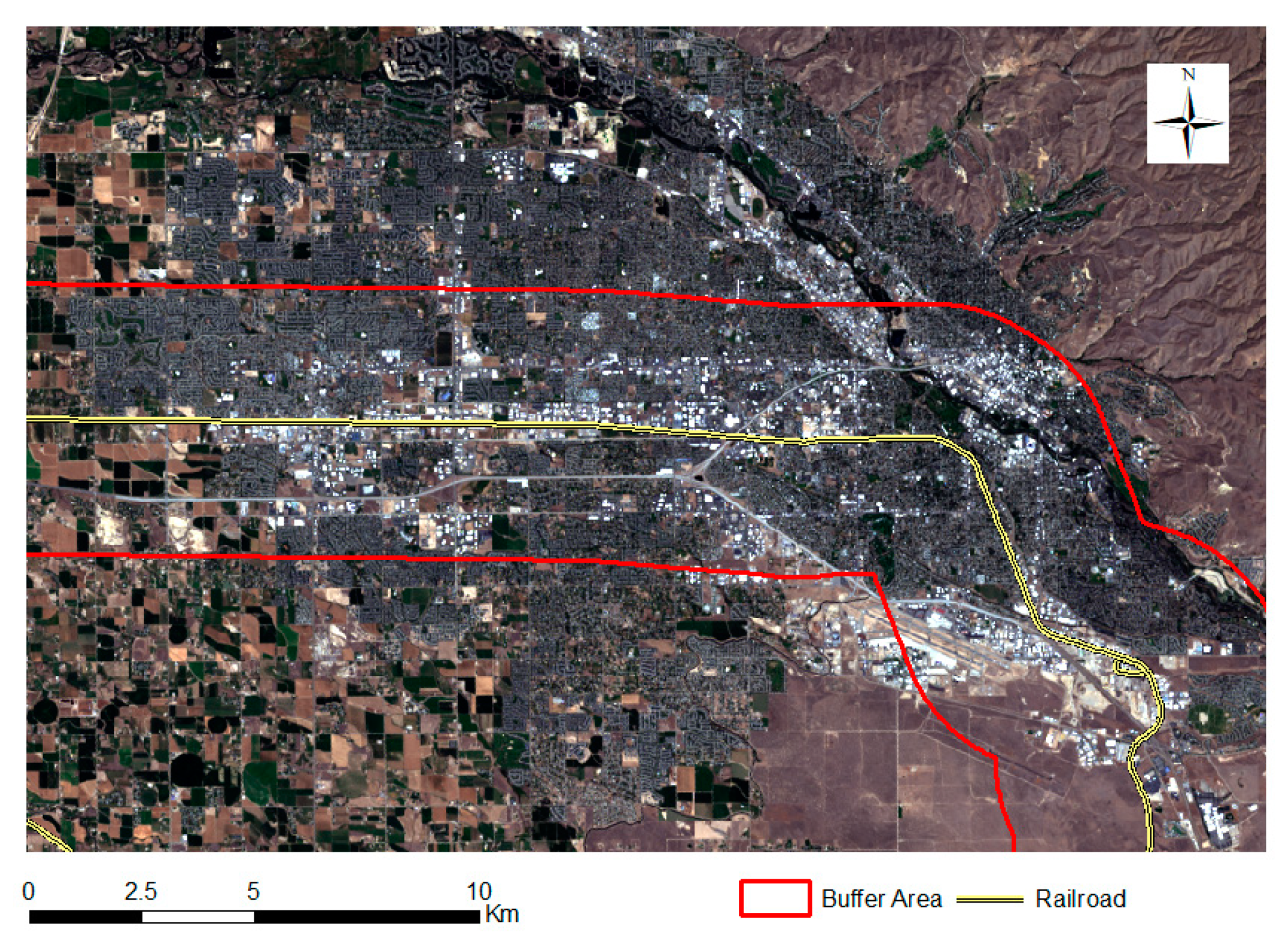
2.1. Study Area

Our study focuses on the Boise-Meridian metropolitan region with a total population of more than 236,000 in 2017 [22] (Figure 1). Located in Southwestern Idaho, this region is characterized by a semi-arid climate. The annual temperature ranges from −4.4 to 33.9 °C with an average high and low temperature above 27.8 °C and below 8.3 °C, respectively [23]. On average, Boise has 206 sunny days per year with an average rainfall of 13 inches. The LULC types in the region include residential, commercial, agriculture, grassland, pasture, water, and open soil. This area has experienced rapid urban growth over the last three decades. With a dramatic influx of population since the 1990s, a large amount of agricultural land has been converted into urban, causing significant changes in the land cover pattern [24].

2.2. Data Processing and Analysis

We obtained two Landsat Thematic Mapper (TM) images and one Landsat OLI/TIRS image from the USGS Earth Explorer website. The Landsat TM images were acquired on July 22nd of 2001 and July 18th of 2008, respectively. The Landsat OLI/TIRS image was acquired on July 23rd of 2013. The three years were selected for comparison because they were all dry years with similar climate conditions. The images were acquired at summertime during dry seasons to minimize the climate and phenological effects. All images were preprocessed involving radiometric and geometric correction.
Vegetation and built-up areas are important land cover types that impact the surface temperature variations. We used the normalized difference vegetation index (NDVI) and normalized difference built-up index (NDBI) to represent the abundance of green vegetation and built-up areas, respectively (Equation (1)). The NDVI is widely used to extract green vegetation biomass and has applications in a variety of fields including LULC change [25], agriculture mapping [26], UHI studies [27], and phenological studies [28]. The NDBI also has widespread evidence supporting its effectiveness in identifying built-up areas [29,30,31]. Both indices were computed based on the spectral reflectance maps created for the three years.
NDVI = ρ ( N I R ) ρ ( R ) ρ ( N I R ) + ρ ( R )
NDBI = ρ ( M I R ) ρ ( N I R ) ρ ( M I R ) + ρ ( N I R )

2.3. LST Retrival

Thermal bands of the Landsat TM and OLI/TRS images were used to retrieve the LST using the single-channel algorithm [32]. The top-of-atmosphere radiance was first converted to the brightness temperature ( T s )
T s = K 2 ln ( K 1 L λ + 1 )
L λ = G r e s · D N + B r e s
where T s is the brightness temperature, and K 1 and K 2 are calibration constants. L λ is the at-sensor spectral radiance calculated from Equation (4). DN is the digital number of each pixel. G r e s and B r e s are the band-specific rescaling gain and bias factor, respectively.
The value of the land surface emissivity ε is obtained from
ε = ε v · P v + ε s ( 1 + P v ) + C
C = ( 1 ε s ) · ε v · F · ( 1 P v )
P v = ( N D V I N D V I m i n N D V I m a x N D V I m i n ) 2
where ε v and ε s are the default emissivity values for vegetation (0.99) and soil (0.96) [33]. C was used to calibrate the cavity and F is the geometrical factor (0.55). P v denotes the proportion of vegetation in each pixel. The value of P v was determined based on the NDVI score of the focal pixel and the maximum and minimum NDVI scores of the map.
Finally, the LST is given by
LST = γ · [ ε 1 · ( ψ 1 · L λ + ψ 2 ) + ψ 3 ] + δ
ψ 1 = 1 τ ,   ψ 2 = L L τ , ψ 3 = L
where L λ and ε are the spectral radiance and the land surface emissivity obtained from Equations (4) and (5) respectively. ψ 1 , ψ 2 , and ψ 3 are the atmospheric functions to correct for atmospheric effects. τ is the atmosphere transmissivity, and L and L are the down-welling and up-welling atmospheric radiance respectively. The values of τ , L , and L were obtained from the atmospheric correction parameter calculator [34]. The values of γ and δ are given by
γ = { C 2 · L λ T s 2 [ λ 4 · L λ C 1 + 1 λ ] } 1
δ = γ · L λ + T s
where C 1 and C 2 are Planck’s constants ( C 1 = 1.191 × 10 8   W · μ m 2 · m 2 · sr 1 and C 2 = 1.43877 × 10 4   μ m · K ). λ is the wavelength of the specific thermal band. The retrieval of the LST was performed in ArcMap 10.6.

2.4. Urban–Rural Gradient Analysis

The transect based method provides a long-range directional assessment of the development pattern and allows more flexibility in capturing uneven urban growth characteristics [35]. It was chosen over other sampling strategies in accordance with the unique growth pattern of the Boise metropolitan area (see detailed discussion in Section 4.3).
We created multiple LST profiles along the urban–rural gradients to understand the spatial variations in the LST across the region. Starting from the center of the city, we created an array of grids that extends towards the edges of the city along four different directions: north–south, west–east, northeast–southwest, and northwest–southeast. The size of the grid was determined as 270 m × 270 m based on prior studies and a series of trial-and-error tests [36]. We extracted the mean LST for each grid and created the LST profiles along the four urban–rural transects for three years.

2.5. Spatial Pattern Analysis

The land composition and spatial configuration of land cover features are key determinants of the LST. While land composition focuses on the abundance and diversity of land cover features, spatial configuration refers to the position, orientation, and spatial arrangement of land cover patches [18]. Considering the drawback of the landscape metrics described previously, we hereby adopted a continuous landscape modeling approach to characterize the abundance and spatial configuration of land cover features respectively.
Spatial autocorrelation indices were used to quantify landscape patterns. We used the Getis-Ord G to represent land cover abundance as it measures the degree of local concentration for a variable of interest. The Getis-Ord G is defined as the ratio of the sum of attributes within a predefined neighborhood to the sum of attributes of all the observations in the study area [37]. The Getis-Ord G statistic for a pixel at location i is given by:
G i * ( d ) = j w i j ( d ) x j j x j
where x j is the attribute value at location j. w i j ( d ) is a binary spatial weights matrix, which defines the neighborhood of the focal pixel. The radius distance d was set as 150 m following a number of prior studies using the Getis statistic for the same purposes [17,19,36,38]. The spatial weights matrix was row-standardized for computation and interpretation. Assuming a normal distribution, the Getis statistic was further standardized by subtracting the expectation from the original value and dividing it by the standard deviation. A high value of G indicates a spatial clustering of high scores and a low value of G indicates a spatial clustering of low scores. Both the high and low values are respective to the mean value of the image. The G statistic was calculated using the NDVI and NDBI maps to represent the abundance of green vegetation and built-up areas respectively (Figure S1).
The degree of spatial clustering is another important spatial character. We used another spatial autocorrelation index—the local Moran’s I to quantify this property [39]. The local Moran’s I denotes the extent of spatial clustering of similar values around the observation i:
I i ( d ) = n ( x i x ¯ ) i ( x i x ¯ ) 2 j w i j ( d ) ( x j x ¯ )
where x i is the attribute value at location i. n and x ¯ are the total number of pixels and the mean pixel value of the image. The same spatial weights matrix specified in the G statistic was used here with the same radius distance. Unlike the G statistic, the local Moran’s I can differentiate a spatially clustered pattern from a spatially dispersed pattern. Specifically, a high, positive local Moran’s I score indicates a highly clustered spatial pattern, while a low, negative local Moran’s I score indicates a highly dispersed spatial pattern. The attribute values used to calculate the local Moran’s I are not as relevant because it is the different spatial arrangement patterns that yield different Moran’s I scores. That said, although the NDVI maps were used to calculate the local Moran’s I, the output maps were not an indicator of vegetation clustering only, but rather the spatial clustering of all land cover features in the region (Figure S1). Note that the local Moran’s I is particularly effective in identifying the spatial pattern of extreme (high or low) values, making it highly sensitive for evaluating the patterns of green vegetation and built-up features.

2.6. Statistical Analysis

A total of 500 random samples were selected for the statistical analysis. We performed the Spearman’s correlation analysis to understand the relationship between the LST and the three spatial autocorrelation indices—G of NDVI, G of NDBI, and local Moran’s I of NDVI. Next, we created pairwise scatterplots to further examine the nature and direction of the relationships. The scatterplots coupled with formal statistical tests collectively determined the final set of predictor variables to enter the multiple regression models.
Spatial dependence exists in any kind of modeling of spatial observations. Regardless of the form of spatial dependence (spatial lag/error dependence), the regularity conditions of the conventional ordinary least squares (OLS) estimation are no longer valid, leading to biased and/or inefficient estimation. Instead of the OLS, the spatial autoregressive models were employed to correct for the spatial dependence among the observations. A specification search was first conducted to determine the form of spatial dependence. Next, the corresponding spatial autoregressive model was specified and fit to obtain the parameter estimates. The Akaike information criterion (AIC) score for both the spatial and linear models was computed. We also reported the pseudo R2, which is the squared correlation between the predicted and observed scores on the dependent variable.
We obtained the LULC maps from the national land cover database (NLCD) to understand the linkage of the LST variations with the urbanization pattern in the region (Figure 2). For each LULC type, we calculated the area change and rate of change from 2001 to 2013. The mean LST for the three years was also extracted for major LULC types.

3. Results

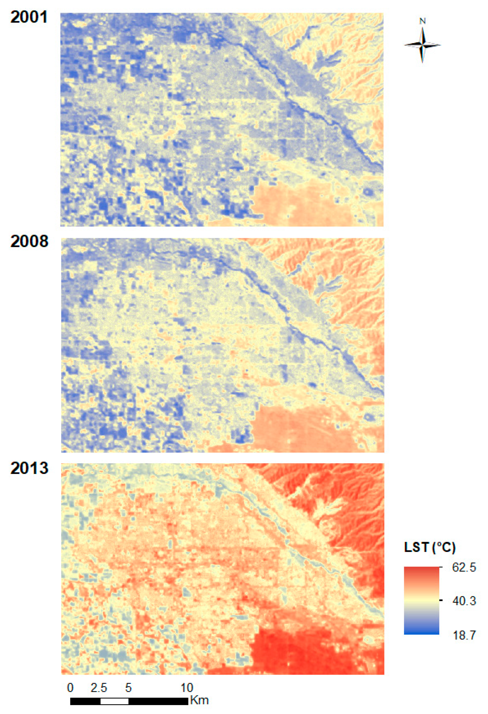
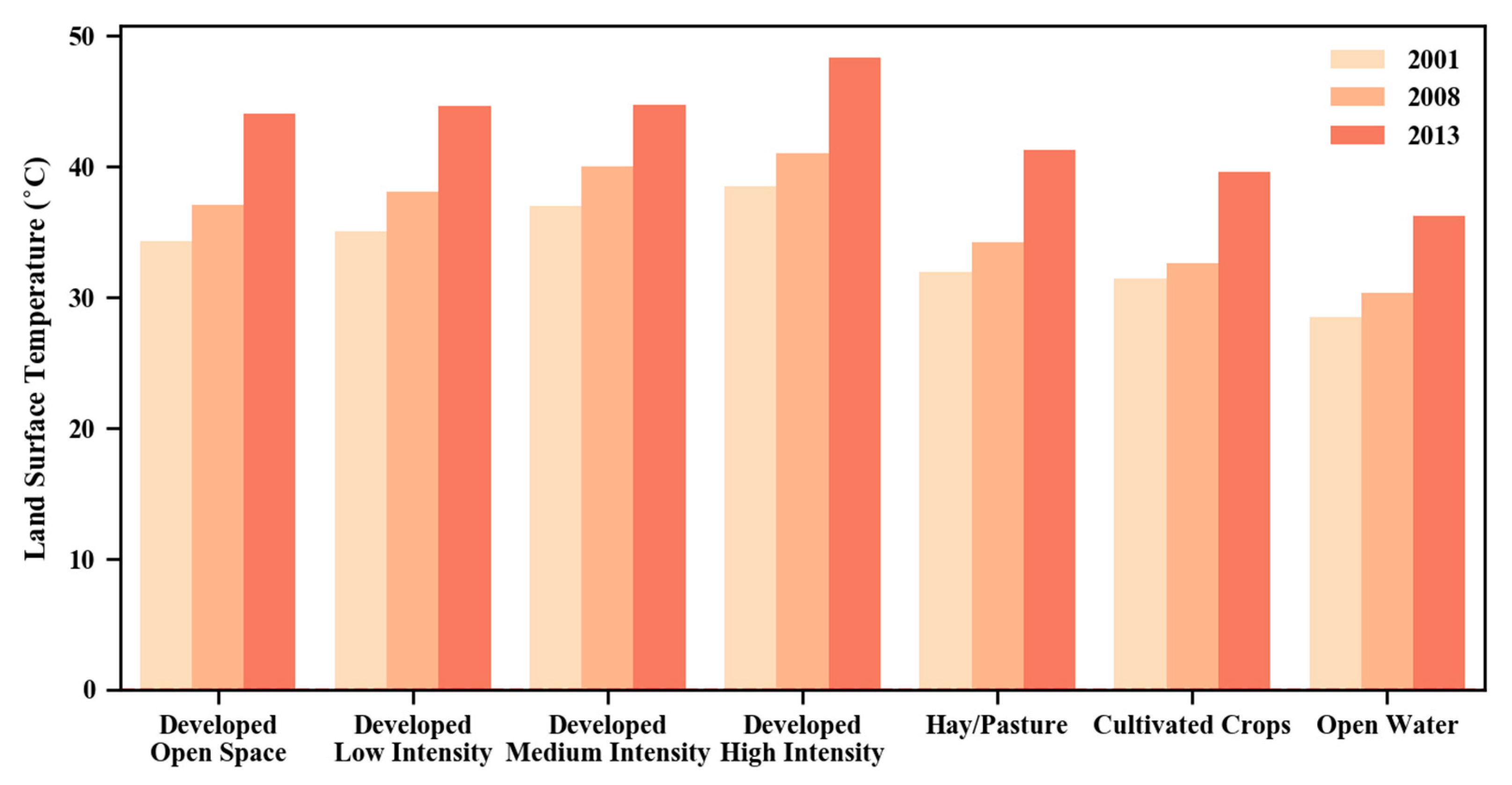
3.1. Spatiotemporal Patterns of the LST

Figure 3 shows the LST maps of the Boise-Meridian metropolitan area in 2001, 2008, and 2013. There was a significant increase in the LST over the whole study area. The average LST increased from 35.6 °C in 2001 to 38.5 °C in 2008, and to 45.8 °C in 2013. Aside from an overall elevation of the LST, dramatic temperature increases were observed for several particular areas including most developed areas, croplands, and herbaceous and shrub/scrub areas in East Boise.

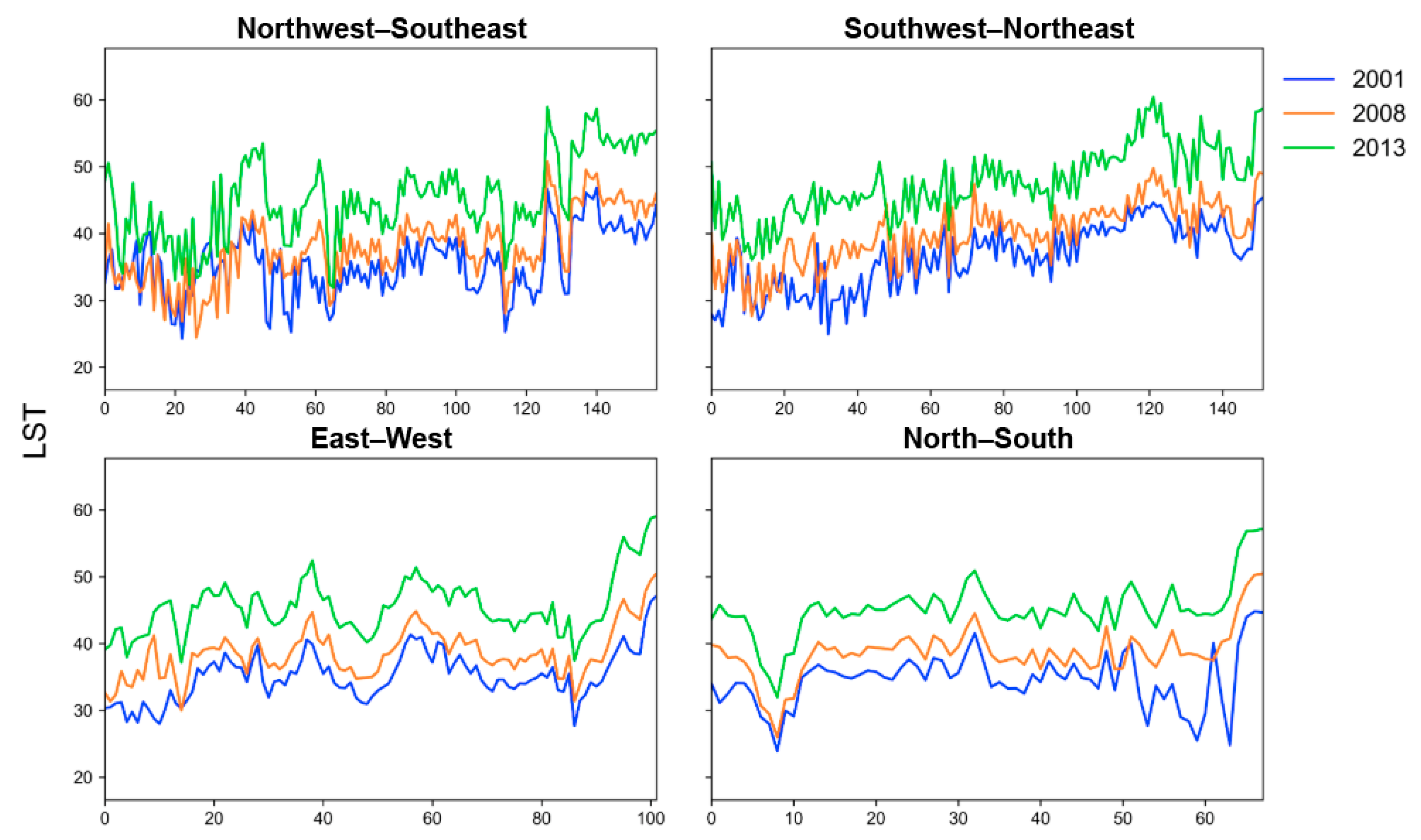
3.2. LST Profiles along Urban–Rural Transects

Figure 4 shows the LST profiles along the urban–rural transects. Regardless of the direction of the transect, all profiles suggested a continuously increasing LST from 2001 to 2013. There was a larger LST increase from 2008 to 2013 than that from 2001 to 2008, indicating a greater warming rate in more recent years. Note that the LST profiles along the diagonals were more volatile than those along the horizontal and vertical directions. This might be due to a diversity of LULC types that diagonal gradients traversed (e.g., agriculture, urban, and herbaceous) compared to the horizontal and vertical profiles (mainly urban). In spite of the volatility, we noticed an overall increasing pattern in the diagonal LST profiles, which again might be associated with the varying LULC types along the gradients. From northwest to southeast (southwest to northeast), the land use type changed from agriculture to developed areas, and to desert landscapes, signifying a gradual temperature increase. The horizontal and vertical profiles were stable across the gradient. There was a rise at the end of the profiles possibly due to a LULC change from urban to desert.

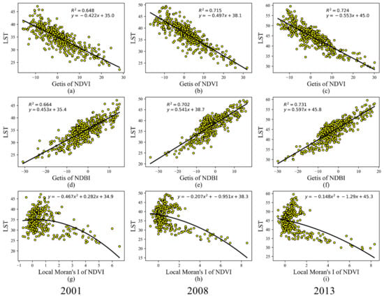
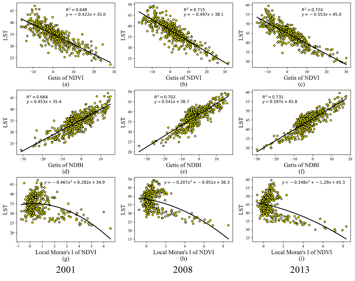
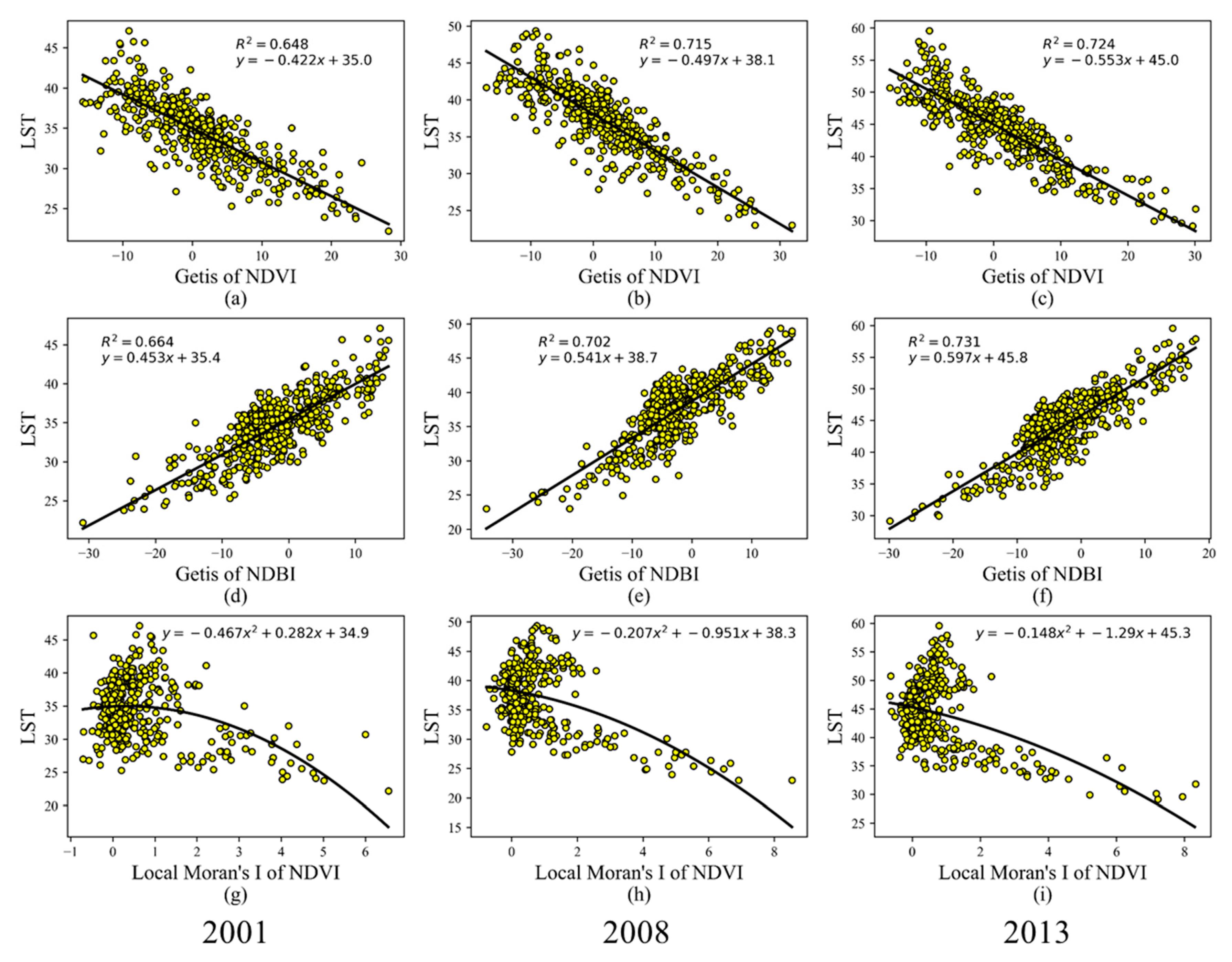
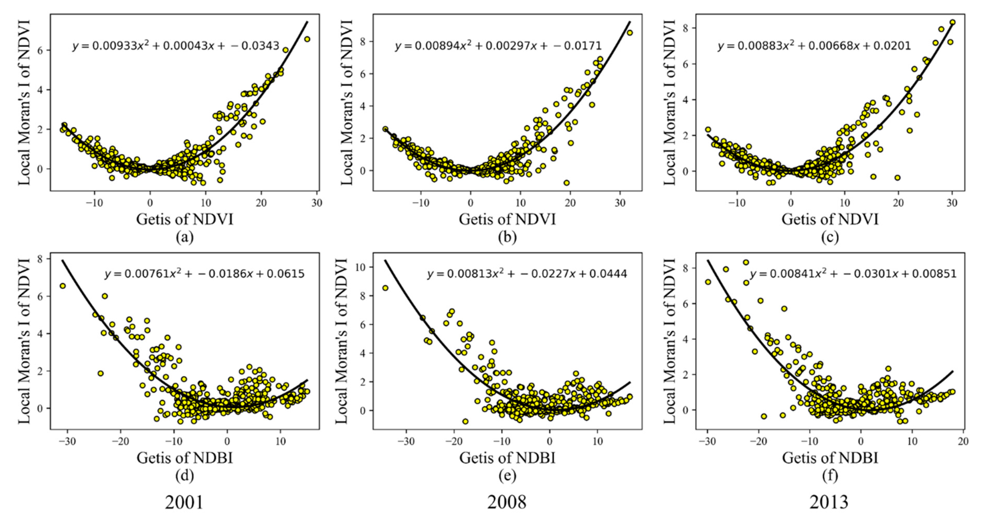
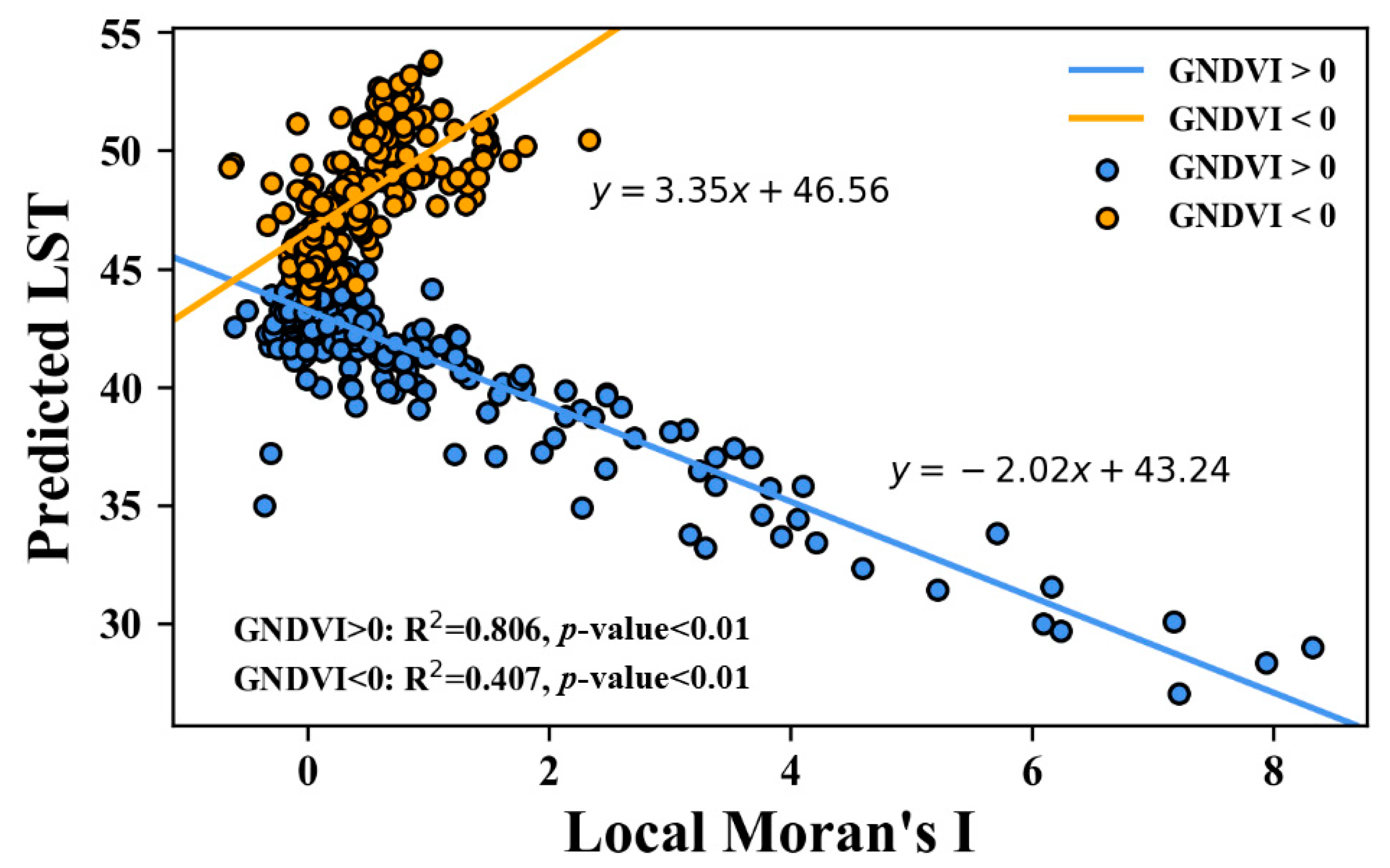
3.3. Bivariate Relationship between LST and Spatial Autocorrelation Variables

Table 1 shows the Spearman’s correlation of LST with the three spatial autocorrelation indices for 2001, 2008, and 2013. All correlations were statistically significant except for the one with the local Moran’s I for 2001. A strong negative relationship existed between the LST and G of NDVI, and the relationship became stronger over time. In contrast, a positive correlation existed between the LST and G of NDBI with a slight increase over the 13 years. There was a significantly negative relationship between the LST and local Moran’s I in 2008 and 2013, but the correlation was much weaker compared with the other two indices.
Since the use of correlation alone may not be able to identify the relationships correctly, bivariate scatterplots were created to better understand the nature and strength of the relationships. Figure 5 shows the scatterplots of the LST with the three spatial autocorrelation indices for the three years. A strong negative linear relationship was identified between the LST and G of NDVI (Figure 5a–c). The relationship was stronger over time based on the size of the regression coefficient. All three models achieved a good fit with the R2 greater than 0.6.
Consistent with the correlation analysis, there was a strong positive relationship between the LST and G of NDBI (Figure 5d–f). Again, the relationship became stronger over time indicated by the increasing regression coefficient. Like the G of NDVI, the G of NDBI was a good predictor of the LST with the R2 greater than 0.65.
The scatterplots of the LST with the local Moran’s I of NDVI showed interesting patterns, which were not revealed by the Spearman’s correlations (Figure 5g–i). For all years, the relationship deviated from a strictly monotonic pattern, and both the first- and second-order models failed to trace the pattern well. There appeared to be a negative relationship for the samples with the local Moran’s I score greater than 2. This indicates that for land cover features exhibiting a higher level of spatial clustering, the degree of clustering might be negatively related to the LST. This statement, however, is tied to the type and abundance of the land cover features, warranting a multiple regression analysis.

3.4. Impacts of Spatial Autocorrelation Indices on the LST

The Lagrange multiplier (LM) test was first employed to determine the form of spatial dependence. In all three years, the Moran’s I score was statistically significant indicating the existence of spatial effects among the observations (results not shown here). Based on the specification search [40], a spatial error specification was determined to be appropriate for all three models.
Table 2 shows the parameter estimation and diagnostics for the spatial error models. We reported the original regression coefficient along with the standard error and statistical significance for each estimation. The standardized coefficient was also calculated to evaluate the relative contribution of each predictor variable to the LST. The variance inflation factor (VIF) for the three models were all below 5 indicating that multicollinearity was not a major concern and that the estimated coefficients were quite stable. The spatial models provided a very good fit for the data as shown by the pseudo R2 scores (≥0.7). Compared to the conventional OLS regression, the spatial models achieved a better prediction accuracy with lower AIC scores.
Based on the results, all three spatial autocorrelation indices were related to the LST, and the relationships were statistically significant except for the one with the local Moran’s I in 2001. The negative relationships between the LST and G of NDVI persisted after controlling for the other variables, so did the significantly positive association with the G of NDBI, which grew over time. Consistent with the correlation analysis, the local Moran’s I was negatively associated with the LST in 2008 and 2013. Based on the standardized coefficients, the G of NDBI had a greater impact (positive) on the LST than the G of NDVI (negative). In spite of the significant relationships with the local Moran’s I, its impact on the LST was minimal after controlling for the other two indices.

4. Discussion

4.1. Changing Climate in Boise

Like many other cities across the globe, Boise has experienced a dramatic temperature increase over the last few decades. According to a national study of temperature change from 1970 to 2018, Boise was ranked as the 13th fastest-warming city in the US [41]. The heating trend has significant impacts on the social, ecological, and environmental conditions in the region. Based on the climate risk assessment conducted by the Langdon Group and the University of Idaho, the frequency of heat stress days with moderate risk will increase from 16 days (historical baseline) to 66 days each summer by 2050 [42]. This is going to have an adverse impact on the population susceptible to heat-related diseases. A moderate drought is projected to occur every two years by the mid-21st century, compared with one in four years now. In addition, the frequency of exceptional drought will increase from one in every 12 years now to one in every three or four years. Further, the odds of very large wildfires in the region will increase by 400% by 2050, suggesting great potential and concerns for chronic air-quality issues within the Treasure Valley.
Our results indicate a major rise in the surface temperatures from 2001 to 2013. The mean LST in the region had increased by 2.9 °C from 2001 to 2008, and by 7.3 °C from 2008 to 2013, resulting in a total of a 10.2 °C increase over the 13 years. There is a greater rate of temperature increase for more recent years than a decade ago, and the trend is consistent for all land use types in the region. The warming trend is evident across the whole study area, but more prominent warming is seen in developed medium and high intensity areas, hay/pasture, and desert lands in East Boise.

4.2. The Interacting Effect of Land Cover Abundance and Spatial Pattern on the LST

While the type and composition of land cover features are key determinants of the LST, the landscape pattern offers additional insight on useful strategies for heat island mitigation. To further explore how the landscape pattern changes with different levels of land cover abundance, we created scatterplots of the local Moran’s I with G of NDVI and G of NDBI respectively (Figure 6). Interestingly, although the local Moran’s I was not a very strong predictor for the variations in LST, there was a concave quadratic relationship of the local Moran’s I with both the Getis variables for all three years. A possible interpretation is that at a lower level of spatial concentration, an increase in the quantity of the land cover (increased Getis) results in a higher degree of landscape fragmentation (decreased local Moran’s I). When the quantity of land cover exceeds a critical point, a continued increase in the land cover abundance will cause the land cover features to cluster (increased local Moran’s I). For both vegetation and built-up areas, the critical point is met when the Getis score approximates zero. Since the Getis was standardized with respect to the mean value, a critical point is reached when the degree of land cover concentration approximates the region average.
Given the findings above, we speculated that the land cover abundance and spatial pattern should be linked to the LST in an interactive manner. Our hypothesis is that the local Moran’s I is statistically associated with the LST with a moderating effect from the Getis variable. In other words, the relationship of the LST with the local Moran’s I varies for different Getis scores. To test this hypothesis, we performed a hierarchical multiple regression and conducted an F test to evaluate the existence of an interaction effect of the local Moran’s I and G of NDVI on the LST. To alleviate multicollinearity, all the predictors were centered by subtracting the mean from the original value. We performed the analysis for three years and the results were reported for 2013 only.
Test results show that adding the interaction term results in a 0.009 change of the R square and a 20.449 change of the F value. The change was statistically significant at the 0.05 level, indicating that the interaction effect from the local Moran’s I and G of NDVI accounted for a significant amount of variance in the LST above and beyond the first-order effect.
To better understand the interacting effect, we created an interaction plot of the predicted LST against the local Moran’s I, using the G of NDVI as the moderating variable (Figure 7). The samples were divided into two subgroups based on the G of NDVI scores: group 1 (blue) has a G of NDVI above 0 and group 2 (orange) has a G of NDVI below 0. The G of NDVI serves as a proxy of a specific land composition scenario. For example, when the G of NDVI is less than 0, the level of vegetation concentration is below the region average, and vice versa. A regression line was fit for each subgroup.
According to Figure 7, the samples were divided into two distinct groups based on the G of the NDVI score. There was a negative relationship of the predicted LST with the local Moran’s I for the subgroup with the G of NDVI above zero. The relationship turned positive for the subgroup with the G of NDVI below zero. Both relationships were statistically significant and the subgroup with the G of NDVI above zero achieved a better model fit (R2 > 0.8) than the other subgroup (R2 > 0.4).
The plot revealed interesting findings regarding optimal landscape designs to cool the city. When the green vegetation abundance is above the region average (G of NDVI > 0), a clustered spatial arrangement is more desirable than a dispersed pattern. This applies to areas such as low intensity developed lands, developed open space, cultivated crops, and hay/pasture. In these areas, planning clumped greenspace is more effective for lowering the surface temperatures. This finding is in line with several previous studies focusing on the spatial arrangement of green vegetation for cooling [8,12,19,43]. A few of these studies, however, have considered the moderating effect of land cover abundance on the relationship between landscape patterns and LST.
When the abundance of green vegetation is below the region average (G of NDVI < 0), the local Moran’s I was positively related to the LST, suggesting that a dispersed landscape pattern is desirable for cooling. Specific land use types in this category include medium to high intensity developed areas, herbaceous, and shrub/scrub. Due to the low coverage of green vegetation, these areas tend to be warmer than the rest of the region. A dispersed spatial arrangement of buildings, for example, could help cool down some of the hottest areas such as those surrounding the Boise airport and downtown Boise. A similar result was reported in a case study in Phoenix, AZ that when controlling for the fraction, clustered paved surfaces result in an aggregate warming effect [14]. This finding was corroborated in a more recent study for Bangkok, Jakarta, and Manila, in which a positive correlation was found between the LST and an aggregation index of impervious surfaces, suggesting a warming (cooling) effect from clustered (dispersed) impervious surfaces [44].

4.3. Urbanization Impacts on the Spatiotemporal Pattern of LST

The Boise-Meridian metropolitan area originally developed along the railroads running across the cities. Railroads attracted commerce and industry to the region in the late 19th and early 20th centuries, which fundamentally affected the growth patterns of the urban areas. Figure 8 shows a satellite image of the region in 2013 together with the railroads and a three-kilometer (two-block distance) buffer along the railroads. Of all the developed areas in the study area, the railroad buffer contains 80% of the high intensity developed areas and 70% of the medium intensity developed areas. From 2001 to 2013, 71.1% of the area increase in the high intensity developed areas occurred in the buffer. This indicates that the urban development occurred mostly along the railroads within a two-block buffer distance.
To analyze the urbanization pattern by LULC type, we created the bar charts showing the area and rate of change for major LULC types in the region (Figure 9). There was a continued growth in the urban areas and a continued decline in the agricultural lands. About 13% of cultivated crops and 5% of hay/pasture were converted into urban. Although the high intensity developed areas took the least land proportion in 2001, its area increased by 66.2% from 2001 to 2013, followed by medium intensity (30.8%) and low intensity developed areas (7.1%).
To better understand the impact of the LULC change on the LST, we created a bar chart showing the mean LST by the LULC type (Figure 10). Consistent across all the LULC types, there was an ever-increasing trend in the LST from 2001 to 2013, with a greater LST increase from 2008 to 2013. The LULC type with the highest LST was the high intensity developed areas, followed by medium and low intensity developed areas, and developed open space. By 2013, the mean LST in all developed areas had reached 44.8 °C and the mean LST in the high intensity developed areas were as high as 48.4 °C.

5. Conclusions

The changing climate has been a major concern as cities continue to expand and intensify. Understanding the trajectories of climate change provides a first step for addressing the key issues city residents are facing in the context of urban warming. Our study presented a spatiotemporal study of the UHI effect in the Boise-Meridian metropolitan area. We employed multitemporal satellite imagery, spatial autocorrelation indices, and statistical analysis to evaluate the changes in the surface temperatures and linked them with the LULC change in Boise from 2001 to 2013.
Results show that even for medium-sized cities like Boise, the urban warming effect had been phenomenal with an average LST increase of 10.2 °C from 2001 to 2013. The warming was confirmed for all the LULC types even for agriculture and open water. Along with the warming there was a major land conversion from agricultural lands into developed areas. Over the 13 years, the area of high intensity developed lands had increased by 66.2% at the cost of a 13% decline in cultivated agriculture.
Our statistical analyses identified a cooling effect from green vegetation and a warming effect from built-up areas, both of which had intensified over time. We found that the warming effect from the built-up features outweighed the cooling effect from the green vegetation. As many agricultural lands are being converted into developed areas during the urbanization, increasing greenspace is among the top priorities for combating the heat. In 2019, a new platform named Boise Climate Now was introduced by the city of Boise to make action plans to mitigate urban warming [42]. A number of action plans were proposed in this platform among which protecting and preserving green and open space was listed as a key target for Boise. In addition to lowering the surface temperatures, increasing vegetation cover such as trees and grass brings many other benefits to the city, including reduced greenhouse gas emissions, better air quality, reduced exposure to the sunlight, and lower energy use.
Our study confirmed the impact of a landscape pattern on the LST, with evidence supporting the additional cooling effect from a clustered spatial pattern of green vegetation. In areas with low vegetation cover, however, a dispersed arrangement of built-up features was more desirable for cooling.
Some other strategies may help mitigate the surface UHI effect. For example, the use of cool roofs and green roofs can help offset the warming effect from urban expansion. Installation of solar panels on roofs has become increasingly popular currently and has been implemented in quite a few cities in the US. The use of solar panels not only lowers greenhouse gas emissions but also helps reduce the solar radiation being absorbed by urban materials, which is the culprit for nighttime UHI.

Supplementary Materials

The following are available online at https://www.mdpi.com/2072-4292/12/10/1631/s1, Figure S1: Maps of G of NDVI (a,d,g), G of NDBI (b,e,h), and local Moran’s I of NDVI (c,f,i) for 2001, 2008, and 2013.

Author Contributions

Conceptualization, C.F.; Data Curation, Z.W.; Formal Analysis, C.F. and Z.W.; Methodology, C.F. and Z.W.; Writing, C.F.; Review and Supervision, C.F. All authors have read and agreed to the published version of the manuscript.

Funding

This research was supported by the Seed Grant from the Office of Research and Economic Development at the University of Idaho.

Conflicts of Interest

The authors declare no conflict of interest.

References

  1. United States Environmental Protection Agency, Heat Island Impacts. Available online: https://www.epa.gov/heat-islands/heat-island-impacts (accessed on 7 February 2020).
  2. Myint, S.W.; Zheng, B.; Talen, E.; Fan, C.; Kaplan, S.; Middel, A.; Smith, M.; Huang, H.-P.; Brazel, A. Does the spatial arrangement of urban landscape matter? Examples of urban warming and cooling in Phoenix and Las Vegas. Ecosyst. Health Sustain. 2015, 1, 1–15. [Google Scholar] [CrossRef]
  3. Tran, D.X.; Pla, F.; Latorre-Carmona, P.; Myint, S.W.; Caetano, M.; Kieu, H.V. Characterizing the relationship between land use land cover change and land surface temperature. ISPRS J. Photogramm. Remote Sens. 2017, 124, 119–132. [Google Scholar] [CrossRef] [Green Version]
  4. Weng, Q.; Lu, D.; Schubring, J. Estimation of land surface temperature–vegetation abundance relationship for urban heat island studies. Remote Sens. Environ. 2004, 89, 467–483. [Google Scholar] [CrossRef]
  5. Yuan, F.; Bauer, M.E. Comparison of impervious surface area and normalized difference vegetation index as indicators of surface urban heat island effects in Landsat imagery. Remote Sens. Environ. 2007, 106, 375–386. [Google Scholar] [CrossRef]
  6. Essa, W.; van der Kwast, J.; Verbeiren, B.; Batelaan, O. Downscaling of thermal images over urban areas using the land surface temperature–impervious percentage relationship. Int. J. Appl. Earth Obs. Geoinf. 2013, 23, 95–108. [Google Scholar] [CrossRef]
  7. Mallick, J.; Rahman, A. Impact of population density on the surface temperature and micro-climate of Delhi. Curr. Sci. 2012, 102, 1708–1713. [Google Scholar]
  8. Li, X.; Zhou, W.; Ouyang, Z.; Xu, W.; Zheng, H. Spatial pattern of greenspace affects land surface temperature: Evidence from the heavily urbanized Beijing metropolitan area, China. Landsc. Ecol. 2012, 27, 887–898. [Google Scholar] [CrossRef]
  9. Maimaitiyiming, M.; Ghulam, A.; Tiyip, T.; Pla, F.; Latorre-Carmona, P.; Halik, Ü.; Sawut, M.; Caetano, M. Effects of green space spatial pattern on land surface temperature: Implications for sustainable urban planning and climate change adaptation. ISPRS J. Photogramm. Remote Sens. 2014, 89, 59–66. [Google Scholar] [CrossRef] [Green Version]
  10. Rhee, J.; Park, S.; Lu, Z. Relationship between land cover patterns and surface temperature in urban areas. GIScience Remote Sens. 2014, 51, 521–536. [Google Scholar] [CrossRef]
  11. Connors, J.P.; Galletti, C.S.; Chow, W.T. Landscape configuration and urban heat island effects: Assessing the relationship between landscape characteristics and land surface temperature in Phoenix, Arizona. Landsc. Ecol. 2013, 28, 271–283. [Google Scholar] [CrossRef]
  12. Fan, C.; Myint, S.W.; Zheng, B. Measuring the spatial arrangement of urban vegetation and its impacts on seasonal surface temperatures. Prog. Phys. Geogr. 2015, 39, 199–219. [Google Scholar] [CrossRef]
  13. Li, W.; Cao, Q.; Lang, K.; Wu, J. Linking potential heat source and sink to urban heat island: Heterogeneous effects of landscape pattern on land surface temperature. Sci. Total Environ. 2017, 586, 457–465. [Google Scholar] [CrossRef] [PubMed]
  14. Zheng, B.; Myint, S.W.; Fan, C. Spatial configuration of anthropogenic land cover impacts on urban warming. Landsc. Urban Plan. 2014, 130, 104–111. [Google Scholar] [CrossRef]
  15. Gage, E.A.; Cooper, D.J. Relationships between landscape pattern metrics, vertical structure and surface urban heat island formation in a Colorado suburb. Urban Ecosyst. 2017, 20, 1229–1238. [Google Scholar] [CrossRef]
  16. Seto, K.C.; Fragkias, M. Quantifying Spatiotemporal Patterns of Urban Land-use Change in Four Cities of China with Time Series Landscape Metrics. Landsc. Ecol. 2005, 20, 871–888. [Google Scholar] [CrossRef]
  17. Fan, C.; Myint, S. A comparison of spatial autocorrelation indices and landscape metrics in measuring urban landscape fragmentation. Landsc. Urban Plan. 2014, 121, 117–128. [Google Scholar] [CrossRef]
  18. McGarigal, K.; Cushman, S. The gradient concept of landscape structure [Chapter 12]. In Issues and Perspectives in Landscape Ecology; Wiens, J.A., Moss, M.R., Eds.; Cambridge University Press: Cambridge, UK, 2005; pp. 112–119. [Google Scholar]
  19. Fan, C.; Myint, S.W.; Rey, S.J.; Li, W. Time series evaluation of landscape dynamics using annual Landsat imagery and spatial statistical modeling: Evidence from the Phoenix metropolitan region. Int. J. Appl. Earth Obs. Geoinf. 2017, 58, 12–25. [Google Scholar] [CrossRef]
  20. Southworth, J.; Munroe, D.; Nagendra, H. Land cover change and landscape fragmentation—Comparing the utility of continuous and discrete analyses for a western Honduras region. Agric. Ecosyst. Environ. 2004, 101, 185–205. [Google Scholar] [CrossRef]
  21. Kowe, P.; Mutanga, O.; Odindi, J.; Dube, T. A quantitative framework for analysing long term spatial clustering and vegetation fragmentation in an urban landscape using multi-temporal landsat data. Int. J. Appl. Earth Obs. Geoinf. 2020, 88, 102057. [Google Scholar] [CrossRef]
  22. United States Census Bureau. Available online: https://www.census.gov/en.html (accessed on 9 April 2020).
  23. US Department of Commerce, National Oceanic and Atmospheric Administration, National Weather Service. NOAA’s National Weather Service—National Climate. Available online: https://w2.weather.gov/climate/ (accessed on 9 April 2020).
  24. Dahal, K.R.; Benner, S.; Lindquist, E. Analyzing spatiotemporal patterns of urbanization in Treasure Valley, Idaho, USA. Appl. Spat. Anal. Policy 2018, 11, 205–226. [Google Scholar] [CrossRef]
  25. Baeza, S.; Paruelo, J.M. Land Use/Land Cover Change (2000–2014) in the Rio de la Plata Grasslands: An Analysis Based on MODIS NDVI Time Series. Remote Sens. 2020, 12, 381. [Google Scholar] [CrossRef] [Green Version]
  26. Lunetta, R.S.; Shao, Y.; Ediriwickrema, J.; Lyon, J.G. Monitoring agricultural cropping patterns across the Laurentian Great Lakes Basin using MODIS-NDVI data. Int. J. Appl. Earth Obs. Geoinf. 2010, 12, 81–88. [Google Scholar] [CrossRef]
  27. Rani, M.; Kumar, P.; Pandey, P.C.; Srivastava, P.K.; Chaudhary, B.S.; Tomar, V.; Mandal, V.P. Multi-temporal NDVI and surface temperature analysis for Urban Heat Island inbuilt surrounding of sub-humid region: A case study of two geographical regions. Remote Sens. Appl. Soc. Environ. 2018, 10, 163–172. [Google Scholar] [CrossRef]
  28. Soudani, K.; Hmimina, G.; Delpierre, N.; Pontailler, J.-Y.; Aubinet, M.; Bonal, D.; Caquet, B.; de Grandcourt, A.; Burban, B.; Flechard, C.; et al. Ground-based Network of NDVI measurements for tracking temporal dynamics of canopy structure and vegetation phenology in different biomes. Remote Sens. Environ. 2012, 123, 234–245. [Google Scholar] [CrossRef]
  29. Liu, L.; Zhang, Y. Urban heat island analysis using the Landsat TM data and ASTER data: A case study in Hong Kong. Remote Sens. 2011, 3, 1535–1552. [Google Scholar] [CrossRef] [Green Version]
  30. Chen, X.-L.; Zhao, H.-M.; Li, P.-X.; Yin, Z.-Y. Remote sensing image-based analysis of the relationship between urban heat island and land use/cover changes. Remote Sens. Environ. 2006, 104, 133–146. [Google Scholar] [CrossRef]
  31. Baño, D.; Salazar, J.; Delgado, M. Remote Sensing in the Design of Urban Planning Strategies, Case Study Urban Heat Island of the Metropolitan District of Quito, Ecuador. Lat. Am. J. Comput. Fac. Syst. Eng. Esc. Politécnica Nac. Quito Ecuad. 2018, 5, 17–26. [Google Scholar]
  32. Jiménez-Muñoz, J.C.; Sobrino, J.A. A generalized single-channel method for retrieving land surface temperature from remote sensing data. J. Geophys. Res. Atmos. 2003, 108, 4688–4695. [Google Scholar]
  33. Jensen, J.R. Remote Sensing of the Environment: An Earth Resource Perspective, 2nd Edition. Pearson. Available online: https://www.pearson.com/us/higher-education/program/Jensen-Remote-Sensing-of-the-Environment-An-Earth-Resource-Perspective-2nd-Edition/PGM200207.html (accessed on 9 April 2020).
  34. Barsi, J.A.; Barker, J.L.; Schott, J.R. An atmospheric correction parameter calculator for a single thermal band earth-sensing instrument. In Proceedings of the IGARSS 2003—2003 IEEE International Geoscience and Remote Sensing Symposium, Toulouse, France, 21–25 July 2003; Volume 5, pp. 033747721–2520033014. [Google Scholar]
  35. Zhang, S.; York, A.M.; Boone, C.G.; Shrestha, M. Methodological advances in the spatial analysis of land fragmentation. Prof. Geogr. 2013, 65, 512–526. [Google Scholar] [CrossRef]
  36. Myint, S.W.; Brazel, A.; Okin, G.; Buyantuyev, A. Combined effects of impervious surface and vegetation cover on air temperature variations in a rapidly expanding desert city. GIScience Remote Sens. 2010, 47, 301–320. [Google Scholar] [CrossRef]
  37. Getis, A.; Ord, J.K. The Analysis of Spatial Association by Use of Distance Statistics. Geogr. Anal. 1992, 24, 189–206. [Google Scholar] [CrossRef]
  38. Buyantuyev, A.; Wu, J. Urban heat islands and landscape heterogeneity: Linking spatiotemporal variations in surface temperatures to land-cover and socioeconomic patterns. Landsc. Ecol. 2010, 25, 17–33. [Google Scholar] [CrossRef]
  39. Anselin, L. Local indicators of spatial association—LISA. Geogr. Anal. 1995, 27, 93–115. [Google Scholar] [CrossRef]
  40. Florax, R.J.; Folmer, H.; Rey, S.J. Specification searches in spatial econometrics: The relevance of Hendry’s methodology. Reg. Sci. Urban Econ. 2003, 33, 557–579. [Google Scholar] [CrossRef]
  41. Climate Central, AMERICAN WARMING: The Fastest-Warming Cities and States in the U.S. Available online: https://www.climatecentral.org/news/report-american-warming-us-heats-up-earth-day (accessed on 9 April 2020).
  42. Climate Action. City of Boise. Available online: https://www.cityofboise.org/programs/climate-action/ (accessed on 9 April 2020).
  43. Masoudi, M.; Tan, P.Y. Multi-year comparison of the effects of spatial pattern of urban green spaces on urban land surface temperature. Landsc. Urban Plan. 2019, 184, 44–58. [Google Scholar] [CrossRef]
  44. Estoque, R.C.; Murayama, Y.; Myint, S.W. Effects of landscape composition and pattern on land surface temperature: An urban heat island study in the megacities of Southeast Asia. Sci. Total Environ. 2017, 577, 349–359. [Google Scholar] [CrossRef] [PubMed]
Figure 1. Landsat Thematic Mapper (TM) imagery of the study area located in the Boise-Meridian metropolitan region, Idaho. The image is displayed in a false color composite.
Remotesensing 12 01631 g001
Figure 2. Land use land cover (LULC) maps of the Boise-Meridian metropolitan area for 2001, 2008, and 2013.
Remotesensing 12 01631 g002
Figure 3. Land surface temperature (LST) maps of the Boise-Meridian metropolitan area in 2001, 2008, and 2013.
Remotesensing 12 01631 g003
Figure 4. Multidirectional and multitemporal LST profiles along the urban–rural gradients.
Remotesensing 12 01631 g004
Figure 5. Scatterplots of LST with G of NDVI (ac), G of NDBI (df), and local Moran’s I of NDVI (gi) for 2001, 2008, and 2013.
Remotesensing 12 01631 g005
Figure 6. Scatterplots of the local Moran’s I with G of NDVI (ac) and G of NDBI (df) for the three years.
Remotesensing 12 01631 g006
Figure 7. Interaction plot of predicted LST with the local Moran’s I for 2013.
Remotesensing 12 01631 g007
Figure 8. Satellite image of the Boise-Meridian metropolitan area in 2013 showing the urban development along the railroads.
Remotesensing 12 01631 g008
Figure 9. (a) LULC area for 2001, 2008, and 2013 and (b) rate of change by the LULC type.
Remotesensing 12 01631 g009
Figure 10. Mean LST by the major LULC type in Boise.
Remotesensing 12 01631 g010
Table 1. Spearman’s rho between LST and the spatial autocorrelation indices for 2001, 2008, and 2013.
YearG of NDVIG of NDBILocal Moran’s I
2001−0.807 *0.767 *−0.075
2008−0.833 *0.779 *−0.152 *
2013−0.837 *0.786 *−0.135 *
* p < 0.05.
Table 2. Parameter estimation and diagnostics for the spatial error model for 2001, 2008, and 2013.
2001
CoefficientStd ErrorStandardized CoefficientVIF
G of NDVI−0.16 *0.031−0.3174.496
G of NDBI0.294 *0.0330.5244.431
Local Moran’s I of NDVI0.1210.113−0.041.313
AIC: 2185.6 (AIC for OLS: 2219.9) Pseudo R2: 0.7
2008
CoefficientStd errorStandardized coefficientVIF
G of NDVI−0.181 *0.024−0.3174.165
G of NDBI0.316 *0.0280.5243.83
Local Moran’s I of NDVI−0.394 *0.09−0.0431.298
AIC: 2177.6 (AIC for OLS: 2188.1) Pseudo R2: 0.77
2013
CoefficientStd errorStandardized coefficientVIF
G of NDVI−0.24 *0.033−0.3694.766
G of NDBI0.319 *0.0340.4574.286
Local Moran’s I of NDVI−0.278 *0.105−0.0621.358
AIC: 2253.4 (AIC for OLS: 2286.6) Pseudo R2: 0.78
* p < 0.05.

