Abstract
Although the real timing and flow rates used for crop irrigation are controlled at the scale of individual plots by the irrigator, they are not generally known by the farm upper management. This information is nevertheless essential, not only to compute the water balance of irrigated plots and to schedule irrigation, but also for the management of water resources at regional scales. The aim of the present study was to detect irrigation timing using time series of surface soil moisture (SSM) derived from Sentinel-1 radar observations. The method consisted of assessing the direction of change of surface soil moisture (SSM) between observations and a water balance model, and to use thresholds to be calibrated. The performance of the approach was assessed on the F-score quantifying the accuracy of the irrigation event detections and ranging from 0 (none of the irrigation timing is correct) to 100 (perfect irrigation detection). The study focused on five irrigated and one rainfed plot of maize in South-West France, where the approach was tested using in situ measurements and surface soil moisture (SSM) maps derived from Sentinel-1 radar data. The use of in situ data showed that (1) irrigation timing was detected with a good accuracy (F-score in the range (80–83) for all plots) and (2) the optimal revisit time between two SSM observations was 2–4 days. The higher uncertainties of microwave SSM products, especially when the crop is well developed (normalized difference of vegetation index (NDVI) > 0.7), degraded the score (F-score = 69), but various possibilities of improvement were discussed. This paper opens perspectives for the irrigation detection at the plot scale over large areas and thus for the improvement of irrigation water management.
1. Introduction
Optimal irrigation relies on an accurate knowledge of plant water consumption, the flow of water, and soil moisture dynamics throughout the growing season. At the plot level, Khabba et al. [1] have shown that better irrigation scheduling can save between 10% and 50% of irrigation water, depending on the irrigation method used and the type of soil. The scheduling and management of irrigation is governed essentially by human decisions, in accordance with various systemic and technical constraints, which are generally unknown at large scales. Globally, 70% of mobilized fresh water is consumed by irrigation and the irrigated surface area of the Earth has doubled over the last 50 years [2]. An adequate understanding and management of this topic is of paramount importance, when it comes to reducing the wastage of water and improving crop yields.
Irrigation scheduling is generally based on a farmer decision-making process, which is used to determine when and how much water should be provided, to optimize the development and yield of the irrigated crops [3,4,5]. Several methods can be applied, to assist the decision-making process used to establish an irrigation schedule such as: (1) water balance simulation models, (2) the monitoring of soil water content or matrix water potential and (3) a combination of both of these. In addition, the farmers ability to follow advice, in terms of dates and quantities of water, can be restricted by several factors: an irrigation infrastructure that imposes the timing of irrigation events, an irrigation method that imposes the volumes of water, the time available to implement scheduling changes, etc.
The in-situ measurement of soil water content is considered to be the best possible measurement technique [6,7]. However, this technology still faces several challenges as for today. On one hand, high-end local measurement point remains expensive but is not able to assess the heterogeneity of soil moisture in a field. On the other hand, a network of sensors (see for example [8]) requires time for installation and maintenance and data management and the system may fail (faulty sensor, incorrect calibration, saving or transfer of data and energy problem with nodes) [9,10].
In this regard, remote sensing products are an alternative for rapid and wider data acquisition [11]. Surface soil moisture (SSM) products derived from active and passive microwave remote sensors have improved over the last forty years [12]. The first mission exclusively designed for the retrieval of SSM was the soil moisture and ocean salinity mission (SMOS) launched in 2009 [13]. It was followed by a second mission named soil moisture active passive (SMAP, [14]). Several other passive and active microwave missions have produced data, which has been used to generate SSM products, such as those provided by the ERS and ASCAT scatterometers [15,16] and AMSR-2 (advanced microwave scanning radiometer [17]). Although SSM products alone are not sufficient for the scheduling of irrigation, several authors have shown that they could be useful for the assessment of irrigation water volumes. Lawston et al. [18] showed that the SSM product derived from SMAP is able to capture irrigation signals over semi-arid regions. Likewise, Malbéteau et al. [19] used 1-km disaggregated soil moisture products derived from SMOS to detect irrigated areas. Using the SM2RAIN algorithm [20], Brocca et al. [21] were the first to use coarse resolution surface soil moisture datasets (from 25 to 40 km spatial resolution, and a revisit time between 1 and 3 days) to estimate irrigation volumes. An interesting aspect of this approach is that the model accounts for underground water losses, which could otherwise be estimated only through the use of an irrigation efficiency coefficient. The same approach was recently applied in Iran [22], and this method has demonstrated its strong potential for the quantification of irrigation, providing good quality of SSM data where there are prolonged periods of low rainfall. Zaussinger et al. [23] also used different coarse resolution datasets and compared them to a water balance, forced by MERRA-2 reanalysis, to determine the use of irrigation water. The statewide comparison showed contrasted results (r between 0.36 and 0.8) and significantly lower estimates than the reported irrigation water withdrawals.
Nevertheless, these irrigation estimations are typically retrieved on a monthly time scale, and for pixels of several km², which is insufficient for irrigation scheduling, in terms of both spatial and temporal resolution. In the last thirty years, synthetic aperture radar (SAR) has shown a high potential to retrieve soil moisture from backscattering coefficients [24,25,26,27,28]. With the recent launch of the Sentinel constellation, several teams have been working on the development of high resolution SSM products, based on the synergetic use of Sentinel-1 radar data, and optical observations from Sentinel-2 or Landsat-8 [29,30,31,32,33,34,35,36]. Greifeneder et al. [37] have also used Sentinel-1 data to detect soil moisture anomalies. The relevant retrieval algorithms are based either on the inversion of a radiative transfer model, or on a machine learning approach. The approach proposed by El Hajj et al. [31] has recently been implemented to produce maps of soil moisture on an operational basis, in different regions of the globe. This work was carried out within the frame of the THEIA program (French land data center, https://www.theia-land.fr), and has for the first time provided the opportunity for irrigation retrieval at the scale of individual fields.
While Earth observation can now provide an estimate of SSM at fine temporal and spatial scales, crop water requirements at the plot scale are commonly estimated by water budget models. The FAO-56 dual crop coefficient model [38,39,40] is a simple and efficient approach for this purpose. The model based on the estimate of water losses due to evapotranspiration (ET). The crop ETc is obtained by modulating the ET of the vegetation of a reference crop (ET0), through the use of a crop coefficient (Kc). Most of the effects of weather conditions are incorporated into ET0, whereas Kc varies according to the characteristics of the crop. The ETc can be reduced according to the water balance to obtain the adjusted ET of the crop (ETcadj). In the dual crop coefficient approach, the ET is partitioned into evaporation (E) and transpiration (T). Since the early nineties [41], the parameter Kc has been related to remotely sensed vegetation indexes. More recently, the relationship between Kc and the vegetation index has been widely studied [42,43,44,45,46,47,48,49]. This combination has been used to develop irrigation scheduling tools [50,51,52,53], which are now reaching a good level of operational reliability, when combined with the 5-day/10 m spatial resolution data provided by the Sentinel-2 A and B constellation. However, the tools that compute a water budget cannot be run automatically, because they rely on user inputs to provide the parameters relevant to their real irrigation schedules.
Our hypothesis is that SSM estimates from SAR remote sensing can be compared to a water budget forced by conventional weather observations in order to detect irrigation events. The objective of this study is to propose a method to make this detection and to assess its performance by comparing in situ and remotely sensed SSM. The study focuses on the detection of irrigation events on irrigated maize with the sprinkler technique in the south-west of France.
The rest of the article is organized in four parts. First, the data and study site are described. Second, the new approach to irrigation retrieval is presented. Third, the results are displayed and analyzed. A discussion identifies some limitations of the method and highlights several potential improvements.
2. Study Site and Data
2.1. Experimental Plots and In-Situ Data
The present study was carried out on six maize plots in South West France, hereafter referred to as P1 to P6 (Figure 1). The region lies in the Oceanic Climate (Cfb in the Köppen classification) of Western Europe but with Mediterranean influences. The soil texture is mostly silt loam, with some variations between plots. These plots were sown with hybrid varieties of maize between April and May 2018. One plot (P1) was not irrigated, three plots were irrigated with rain guns and two plots were irrigated with a center pivot. Sprinkler irrigation systems are well suited for scheduling, as farmers can control their discharge rate, duration and frequency [4]. However, hose-reel systems are not as flexible as solid set systems or pivot or lateral displacement systems, because they are not suitable for very small or large application depths. In addition to the variability of precipitations (rain gauges installed on each plot registered from 229 mm to 452 mm), that is the reason why the irrigation amounts ranged from 8 to 40 mm and the number of irrigations per plot varied between 3 and 10. Sentek Enviroscan probes were installed on each plot, for most of the growing season, and soil moisture measurements were taken at 10 cm depth intervals, between 5 cm and the maximum measurement depth (60 or 90 cm depending on the soil). This data was used to determine the maximum root depth of each plot. The half-hourly measurements at 5 cm were averaged for each day and referred to as SSMsentek to provide data to be comparable to the water balance model described below. The variables needed to compute the reference evapotranspiration (air temperature, dew point and wind speed) were retrieved from the closest weather meteorological organization synoptic station of each plot (http://ogimet.com). The corresponding plot descriptions are provided in Table 1.
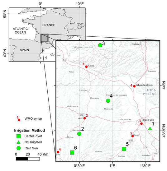
Figure 1.
Location of the six experimental plots in South West France with their corresponding nearest Word Meteorological Organization (WMO) synop stations.

Table 1.
Description of the six experimental plots. Irrigation and precipitation depths are summed between sowing and harvesting.
2.2. Satellite Data
Sentinel-2 is a constellation of two sun-synchronous, multi-spectral imaging satellites, orbiting at an altitude of 786 km, with a 5-day repeat cycle. The Sentinel-2 level-2A product is used to assess the state of vegetation development. The product distributed by European Space Agency (ESA) (https://scihub.copernicus.eu), which provides the bottom-of-atmosphere reflectance and a cloud mask was chosen. Only cloudless dates (i.e., 0% cloud inside the plot) were retained, from which the normalized difference of vegetation index (NDVI) was computed at 10 m spatial resolution, using the reflectance bands 4 (664.6 nm) and 8 (832.8 nm). This data was averaged over each plot. The NDVI was used as a linear proxy for the basal crop coefficient (Kcb, [54]) and fraction cover (Fc, [55]) for maize.
El Hajj et al. [31] used Sentinel-1 and Sentinel-2 time series data to develop an operational neural network for the estimation of surface soil moisture SSM (in the upper 3–5 cm). This product, which is referred to as S2MP (Sentinel-1/Sentinel-2-derived soil moisture product at the plot scale), is computed using the ascending orbits of Sentinel-1, which pass above the corresponding latitudes at around 6 pm. Measurements recorded during the descending orbit, which passes overhead at around 6 am and is often affected by frost or morning dew, were not used. The neural network searches for the best fit to the calibrated water cloud model (WCM) [56], combined with the soil backscattering model integral evaluation model [57]. In the WCM, the total backscattered coefficient is modeled as the sum of the direct vegetation contribution and the soil contribution, multiplied by an attenuation factor. The product accuracy was estimated to be approximately 5.5 vol% for dry to slightly wet soil conditions, and 6.9 vol % for very wet soil conditions. However, its accuracy can decrease if the surface is very smooth (roughness < 1 cm), or very rough (roughness > 3 cm). These authors have also shown that the soil moisture RMSE increases slightly (by approximately 1.5 vol %) when the NDVI increases from 0 to 0.75. When the NDVI is greater than 0.75, the radar signal in both VV and VH polarizations can be characterized by a significant fall in sensitivity to soil moisture. The decrease in accuracy associated with a dense vegetation cover, which also affects the S2MP product, can thus be expected to be found in all products derived from C-band SAR imagery.
The online product is computed and delivered for homogeneous plots based on a segmentation pretreatment and made available there: https://www.theia-land.fr/en/product/soil-moisture-with-very-high-spatial-resolution.
For this study, the calculation was redone for the exact extent of the six plots, producing single time series for each plot P1 to P6. Note that the size of the fields in this study ranged from 4.7 to 26.8 ha meaning that speckle was significantly reduced as 1 ha is about 100 pixels of Sentinel-1. In order to evaluate the quality of the S2MP, the time series were compared to in situ measurements (Figure 2). The S2MP estimates were available at a frequency of 1–6 days, on plots 2–6, and only once every 12 days on plot P1, which was observed by Sentinel-1B only. In order to reduce the noise, consecutive days have been averaged and assigned to the first day. The S2MP product provided values of the same order of magnitude as those derived from in situ measurements. As expected, S2MP did not fit well with local measurements (low r2 and RMSE) when NDVI was over 0.75. However the alternating dry and wet events, which occurred during the middle of the season, close to the period of full crop development seemed well detected by the S2MP. It appeared to be meaningful information to detect irrigation. This is the reason why the algorithm described below was based on change detection, rather than on the measurement of absolute values.
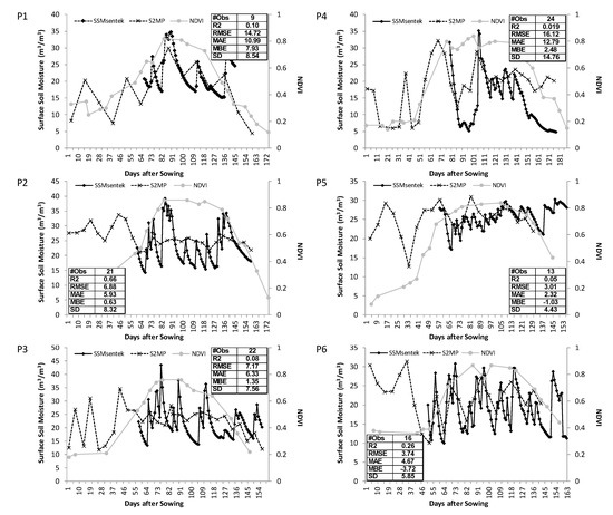
Figure 2.
Time series of surface soil moisture after sowing, for six maize plots. The NDVI is shown in light gray. The tabular insets indicate the number of S2MP observations (#obs), as well as the statistical parameters used to compare S2MP with surface soil moisture (SSM)Sentek: the determination coefficient (R2), the root mean squared error (RMSE), the mean absolute error (MAE), the mean bias error (MBE) and the standard deviation (SD), the last third in m3·m3−1.
3. Method
Irrigation events were estimated by comparing the water budget of the upper layer of soil to the observed SSM. The four steps in our irrigation retrieval algorithm are summarized in Figure 3. They consist of (1) adjusting the timing of the time series, (2) estimating the surface soil moisture at the frequency defined by the daily time step, (3) comparing the model with SSM data, in order to detect irrigation events and (4) determining the best date of irrigation in between two SSM observations. The in situ observations and remotely sensed soil moisture product were tested in this study.
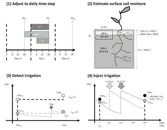
Figure 3.
The four steps used to estimate irrigation dates.
3.1. Step 1—Adjusting from Instantaneous to Daily Values
This adjustment is illustrated in Step 1 of Figure 3. The total rainfall and evapotranspiration were thus computed for each day, and the S2MP product was estimated at the time when Sentinel-1 passes overhead (around 6 pm). In order to synchronize the rainfall and evapotranspiration with the remotely sensed data, it was decided to use 24 h intervals starting at 6 pm on the previous calendar day (j-1) and ending at 6 pm on the current calendar day (j). The daily precipitation of this 24-h interval was then given by the sum of one quarter of the values recorded during the previous calendar day, plus three-quarters of those corresponding to the current day. This approach is similar to that used by Allen [40]. As evapotranspiration occurs mainly during the daytime, between 6am and 6pm, its daily distribution remained unchanged. The resulting irrigations computed for this 24-h period were thus assigned to the current calendar day (j).
3.2. Step 2—Estimation of the Soil Water Content of the Upper Layer
The FAO-56 method [39] was retained since it is extensively used for irrigation scheduling. The following description is based on the implementation described in Le Page et al. [52]. This model was developed specifically for the simulation of evapotranspiration. The transpiration is taken from a bucket of soil expanding from the surface to the root depth (Zr). The root depth growth between 0 and a maximum root depth (Zrmax, see Table 1) linearly to fraction cover (Fc). In this study, the maximum root depth of each study plot was set according to the study of the different soil moisture sensors. Inside this bucket, a second bucket accounted for the evaporation of the non-covered area of soil (1-Fc). The depth of this bucket (Ze) depended on the soil texture, and varied from 7 to 15 cm. In FAO-56, the water content of the evaporation bucket was computed for the fraction of the soil that is both exposed and wetted. This concept is different from a bucket, which would account for the soil moisture of the upper layer of soil (SWCtop), which is the quantity that needs to be compared with the observed SSM values. For this reason, it was proposed to slightly modify the method used by the FAO-56 model according to Raes’ findings [58]. Of the transpiration 40% comes from the first upper quarter of soil (Zr/4). The main bucket was thus divided into two layers, with the upper layer having a depth equal to one-quarter of the root layer. For a maximum depth of 60 cm, this means that the first quarter had a depth ranging between 0 and 15 cm. The lower layer was the complement of Zr, and SWCtop was computed as follows: in Equation (1), the depth of the first quarter of soil was updated according to the new root depth, using a daily time step (j). Drtop is the depletion of water in the upper layer and θfc and θwp are the field capacity and wilting point of the soil. TAWtop and TAWdown correspond to the total available water content in the upper and lower layers, and are computed in the same way as TAW in the FAO-56 model, but are fractioned into the upper (25%) and lower (75%) percentages (Equation (2)). The depletion of the bottom layer Drdown is computed as the difference in depletion between the full root layer and the top root layer.
In a second step (Equation (3)), Drtop is updated in accordance with known wetting events, and depletion is constrained between 0 and the maximum water content TAWtop:
The transpiration of the upper layer is computed from Equations (4) and (5). The stress coefficient of the top layer (Kstop) was computed in the exactly the same way as Ks in the FAO-56 model, but with the water quantities of the top layer (Equation (4)), where padjust is the average fraction of TAW that can be depleted from the root zone before water stress occurs. The transpiration of the top layer (Ttop) was then obtained with the basal crop coefficients Kcb and previously computed Kstop. In accordance with the findings of Raes [58], 40% of the transpiration is affected to the top layer. Ttop cannot be greater than the total amount of transpiration T computed with the regular FAO-56 model (Equation (5)):
Drtop is updated by summing the evaporation (E) and the transpiration (Ttop):
E was previously computed in the same way as in the FAO-56 model, using the evaporation bucket. Note that with shallow roots, the depth of the evaporation layer may be smaller than the upper layer, which can lead to inconsistencies.
This approach distributes the water available in the main bucket into an upper and a lower bucket. However, it does not fully achieve the objective of computing the water budget of the upper layer with a fixed depth of 3–5 cm. Indeed, the depth of the computed layer depends on the root depth Zr. This point is discussed later. Note that some potential water balance terms have been neglected. The simulation of capillary rise was not necessary because there was no shallow aquifer beneath the plots. Runoff was also neglected because it is normally uncommon on well leveled irrigated plots. Likewise deep percolation occurs in case of excess input water in the FAO-56 parameterization. It does not affect the budget of the rooting compartment.
3.3. Step 3—Irrigation Detection
Irrigation is detected with the change detection algorithm described in step 3 of Figure 3, which is based on the soil moisture dynamics between two dates. The SSM provided by the measurements (derived from either in situ or S2PM observations) and the model described in 3.2 are referred to as θobs and θm, respectively. Δθobs nd Δθm are the difference in SSM between the previous (i-1) and current steps (i), for the observations and the model, respectively. Note that the number of days between two steps depends on the timing of the measurements. Since the S2PM product is supposed to be very degraded when NDVI > 0.7 and that was confirmed for our dataset (Figure 2), it is assumed that variations between the model and the measurement are not necessarily compatible in amplitude, only the signs of the change are compared: irrigation could potentially have occurred when Δθobs > 0 and Δθm < 0. Note that this assumption about amplitudes might also be interesting for using uncalibrated sensors. At least two issues arise from this approach: (1) when there are too many days between date i-1 and date i, wetting events (rainfall or irrigation) from the first part of the period will not increase θobs(i) and (2) when θm(i-1) is already dry, the SSM cannot decrease much further so that the condition Δθobs > 0 may not be satisfied due to observation uncertainty. Additionally, little rainfall may be sufficient to cause an increase of SSM (Δθm > 0).
In order to address issue 1, a threshold κ was introduced, in order to account for the number of days between (i-1) and i. Basically, κ represents the minimum increase in SSM (in m3/m3) that can be interpreted as an irrigation event. The threshold is high when the time step is short (e.g., one day) and decreases when the number of days between two measurements increases. Equation (7) provides a simple approach to the modeling of this behavior, where the number 6 is a compromise between the repeat period of Sentinel-1 and the number of days after which an irrigation event would no longer be visible in the SSM data. The coefficient κ is related to the soil texture and must be adjusted:
Issue 2 is addressed through the use of a second threshold Ψ, which is computed empirically from Equation (8), where p is the threshold between readily available water and stress, in accordance with the FAO-56 model (e.g., 0.55 for maize). Ψ increases when θm(i) decreases, and when θm(i) > p, it is equal to zero:
Finally, an irrigation event occurs between dates (i-1) and i, when Δθobs > κ and Δθm < Ψ.
3.4. Step 4: Irrigation Injection
If an irrigation event is detected, the irrigation date is sought between the beginning (day i-1) and the end of the period (day i). This period has a maximum duration of 12 days, with one Sentinel-1 flyover, and typically 6 days with Sentinel-1 A and B flyovers. The water balance was iterated for each day of this period, by injecting a fixed volume of water on each different day. This amount was set according to the known amounts used for the irrigation of each plot (Table 2). It is likely that this approach would not be suitable when the interval between two observations is too long or when the irrigation system is easy to handle (e.g., full coverage irrigation). We identified at least two different objectives for selecting the day j of irrigation injection. If observation and data were reliable, the objective would be to reach the SSM of the observations at the end of the period. Instead, we chose to select that day when the difference in SSM between model and observation at the end of the period is closer to the difference in SSM at the beginning of the period. Finally, the injection date is confirmed only if the model and observation have the same sign of the difference:
where n is the number of days in the period.
Table 2.
Fixed volumes for irrigation injection, derived from real irrigation volumes.
3.5. Accounting
In order to assess the validity of irrigation detection, three classes were proposed according to a timing range n expressed in days. A computed irrigation event was classified as a true positive (TP) if it is detected within a range of ± n days with respect to the observation. If the simulated irrigation does not lie within ± n days of the observed irrigation event, it is classified as a false positive (FP). If the irrigation is missed, or if no irrigation event is retrieved within ± n days of the observed irrigation event, it is a false negative FN. The number of days n was tested with 3 days and 5 days, and the final result was the average of the two tests. The “precision” p = TP/(TP + FP), and the “recall” r = TP/(TP + FN) could then be computed. The F-score, which is the harmonic mean of the precision and recall, was finally computed as: F1 = 2.p.r/p + r. This score that can range between 1 (perfect accuracy and recall) and 0 was multiplied by 100 for presentation purposes.
4. Results
4.1. Analysis of Soil Moisture Changes for the Detection of Irrigation Events
Figure 4 summarizes the 29 irrigation events recorded on the five irrigated plots. The difference in soil moisture between the S2PM dates was computed before and after irrigation, and the change (“delta”) in SSM provided by the model was computed using real irrigation data. The local soil moisture showed 75% and 82% of compatibility with S2PM and the model respectively. The compatibility between S2PM and the model was 71%. Concerning the accuracy with which irrigation events were detected using this method, with the local SSM and S2PM measurements, true positive results were obtained in 59% and 63% of cases, respectively. When delayed detections (within a 6-day interval following an irrigation event) were aggregated, the accuracy climbed to 74% in both cases, which was considered to be the maximum achievable score using the present method and dataset. As revealed by this analysis, various circumstances could lead to incorrect detections: if a second irrigation event occurs within the time interval separating recorded events (events 11, 17, 22 and 26), only one event was accounted for, meaning that with this dataset, the highest achievable accuracy was only 85% (24/29). In cases where the moistening effects of irrigation disappeared during the sampling period (event 20), detection was very random. In some cases (events 4, 7 and 8), an increase in SSM was observed only during the next sampling interval. This was probably caused by misalignment of the data. In some cases, the in situ measurements (events 28 and 29) or S2PM (event 15) appeared to be incorrect. Lastly, irrigation events may in some cases be masked by rainfall (event 14).
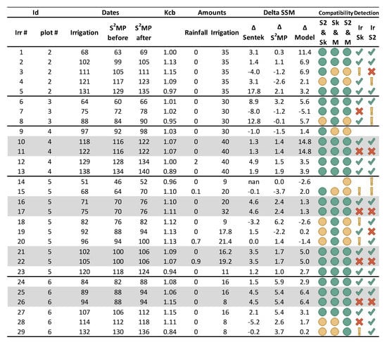
Figure 4.
Summary of each recorded irrigation event: The “compatibility” (same variation) between two sources (S2 for S2PM, Sk for in situ, M for Model) is indicated by a green circle, and a yellow circle on the contrary. In the “Detection” columns, a green tick corresponds to an increase in both SSM, a red cross corresponds to a opposite variation, or impossibility of detection due to the time step of observations. The yellow exclamation mark indicates a possible mismatch with the next time interval. The gray lines indicate when two irrigations occur between two S2PM observations.
4.2. Detection of Water Turns Using In-Situ SSM Measurements
Table 3 lists six different scores (TP, FP, FN, precision, recall and f-score) obtained for each plot, using the in situ SSM for different values of the coefficient k (1,2,3,4), with lapses ranging between one and six days. The last six lines give the scores for the total number of irrigation events. For plot 2, a perfect f-score was obtained despite the fact that the first irrigation event did not produce an increase in SSMsentek. In fact, the irrigation event detected during the following time lapse was accounted for as a TP. This example show that this scoring technique could lead to incorrect conclusions. Another interesting aspect of this table is that for most plots, the most useful time lapses were between 2 and 4 days. A longer (5–6 days) or shorter time lapse (1 day) generally provided worst scores. Additionally, note that the coefficient k seemed to vary from one plot to another, as could be expected, since it represents the time taken for the soil to dry out to the point where the effects of the previous irrigation event become unnoticeable. This parameter varies mainly as a function of soil texture and irrigation volumes. Figure 5 illustrates how the irrigation have been detected on the time series of the six plots. Note that there was no irrigation detection on the non-irrigated plot P1, and that the detections were generally accurate for the five other plots.
Table 3.
Irrigation detection scores using SSMSentek with 1–6 day intervals (rows), with k ranging from 1 to 4 (columns). The last six rows are the scores for the total number (29) of observed irrigation events.
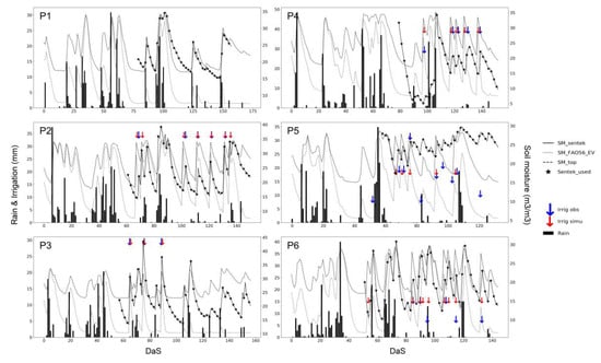
Figure 5.
Irrigation detection for six plots using SSMSentek with a time step of two days and k equal to 2. The soil moisture variables are shown as volumetric percentages (right axis). Rainfall and irrigation events are given in millimeters (left axis). The scale on the horizontal axis corresponds to the number of days since sowing.
4.3. Detection of Water Turns Using the S2MP Product
Figure 6 is very similar to Figure 5, but was produced using SSMS2MP data, from which Table 4 lists the corresponding scores. As the measurement period used for the S2MP data was longer than in the case of the sensor measurements, the scores were adjusted accordingly for the purposes of comparison. In addition, as the Sentinel-1 images are evenly spaced by a period of six days, the coefficient k had no effect here. As stated earlier, it would probably be more appropriate to use a coefficient that takes not only the number of days between measurements, but also the soil texture and irrigation volumes into account.
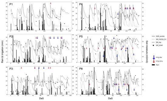
Figure 6.
Irrigation detection for six plots using the S2MP product. The soil moisture variables are shown as volumetric percentages (right axis). Rainfall and irrigation events are given in millimeters (left axis). The scale on the horizontal axis corresponds to the number of days since sowing.
Table 4.
Scores obtained with the S2MP product.
The soil moisture estimations derived from Sentinel-1 data were different to those provided by the in situ sensor measurements, especially when vegetation was close to full cover. In addition, as the remotely sensed data is recorded at six-day intervals, a certain loss in performance could be expected: the average f-score was found to be lower than the best scores obtained with local soil moisture measurements when they were recorded at shorter intervals (2–4 days). However, similar scores were achieved in the case of longer intervals (5 and 6 days). In addition, it is important to note that the reduced performance of the Sentinel-1 estimations can be accounted for mainly by its poor performance on plot #3.
A false positive result was noted on plot #1. As the S2MP product correctly identified an increase in soil moisture due to rainfall, the error can be attributed either to underestimation of the rainfall event, or to the fact that the model did not adequately reproduce the increase in soil moisture. Similar errors were observed at the beginning of the season for plot #5. On the other hand, the false detection of irrigation events on plots #3 and #4 at the beginning of the season were due to an increase in SSM that could not be explained by recorded rainfall amounts.
In general, the recall was found to be much lower than the precision, meaning that there were more missed detections (false negatives) than invalid detections (false positives). As shown in Section 4.1, this outcome was quite predictable, due to the limitations of the algorithm (see Discussion). The true positive score of 17 was thus very satisfactory, in view of the maximum possible score of 22.
4.4. Sensitivity Analysis
The two thresholds of the algorithm were already determined with in-situ sensor data. Figure 7 shows the f-scores obtained for varying rainfall, soil water retention and fixed irrigation amount with the S2SM dataset. Those variables commonly have relatively large spatiotemporal variability and associated uncertainties. White noise, with a Gaussian distribution, corresponding to an error varying from 20% to 80%, was added to the rainfall data of each event. This noise did not affect the timing or length of events. Over the tested range, the performance of the algorithm was only slightly degraded when the noise was increased. Concerning the fixed irrigation amount, its reduction to an amount lower than 20 mm had a larger impact. Increases above this threshold had negligible impact, which was expected for two reasons. First, the algorithm took it into account when determining the irrigation date between two dates. The maximum impact was therefore 6 days for Sentinel-1 data. Secondly, irrigation events higher than 20 mm did not increase the impact on the soil moisture of the upper layer of soil. The sensitivity to the soil retention parameters was analyzed by adding a variability of −0.1–0.1 m3·m−3 to field capacity and half of this variation to the readily available water. The performance was reduced or stable when soil retention was reduced. An increase in performance could however be observed for P2 and P3 when soil water retention was increased, probably meaning that the initial setup should be revised.
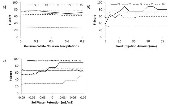
Figure 7.
Sensitivity analysis on precipitation (a), irrigation amounts (b) and soil water retention (c).
5. Discussion
The approach described in this study makes use of the FAO-56 model, combined with remotely sensed observations, as a proxy for crop growth. The FAO-56 dual crop method is designed to estimate evapotranspiration by computing evaporation and transpiration separately. As it is not possible to estimate the SSM using this method, we proposed to distribute the soil moisture over upper and lower compartments. These are apportioned in accordance with the rooting reservoir, so that the depth of the upper (surface) compartment varies as a function of root development. SSM could be better represented with the use of different soil water balance models [59,60]. In this case, one could expect an improvement of the irrigation detections. A simple alternative would be to implement a precalibrated force-restore method [61,62], in parallel with the FAO-56 model. FAO-56 is a single bucket model that includes the Ritchie approach of evaporation [63]. In the models DSSAT [64], BUDGET [58] and AQUACROP [65], the soil profile is divided into several small soil compartments that have their own soil parameters. The differential flow equation is replaced by a set of finite difference equations. The infiltration works as tipping buckets. Drainage is computed between each compartment. The overall transpiration must also be distributed to each compartment according to root density and water stress at each compartment. Mechanistic models using Darcy’s law and continuity equations could also provide an alternative approach. However, Ranatunga et al. [60] note that models based on Richards’ equations assume the soil to be incompressible, non-hysteretic and isothermal, and also make the assumption that soil moisture does not travel through macropores and preferred pathways. It would permit to model the potentially strong soil moisture gradients, and potentially better resolve evaporation. This could also take better advantage of the vertically varying root profile, if this data is available. The disadvantages of both the multilayer and Richards approaches is that they are more complex, and more computationally expensive, so that they may not be appropriate for the detection of irrigation over large areas.
When compared to its optical and thermal counterparts, SAR imagery has the advantage of remaining unaffected by clouds, thus allowing continuous coverage to be achieved. In addition, microwave signals have the advantage of passing through the canopy to a certain extent and penetrating the soil, thus making it possible to obtain an estimation of soil moisture in the first few centimeters of soil. The SSM dataset, based on Sentinel-1 imagery, has the considerable advantage of providing high resolution (10 m) radar scans every six days. However, a large proportion of the backscattered radar signal is produced by vegetation through volume scattering and impacted by soil roughness, which means that the resulting SSM estimations can be somewhat inaccurate, especially when annual crops are well developed or grown under tree coverage. Furthermore, since the dataset indicates that it is not possible to introduce the absolute difference in soil moisture, we used the change of SSM trajectory between model and observation. This approach has proved to be reliable when using in situ observations of SSM. When using the Sentinel-1 product, it also indicates that a repeat time of 2–4 days would be more adequate. As there are currently no SAR frequencies available with a better revisit time than that of Sentinel-1, alternative methods could be considered. As an example, the SWIR band of optical observations could be used to obtain soil moisture estimations for the skin layer.
The parameter k was introduced in an effort to account for variations in the irrigation detection threshold, as a function of soil water content and the interval between two observations. The influence of this threshold was studied with only four values (1, 2, 3 and 4), and its value was found to change considerably from one plot to another. This suggests that the threshold should depend not only on time, but also on soil texture and the volume of irrigation water. In addition, as this threshold could be attenuated when the soil is covered with vegetation, it would be of interest to study its relationship with an index such as the NDVI. A bigger database would also make possible to search for an optimal threshold value. Unwanted irrigation events were detected on P2, P3 and P5 at the beginning of the season. A rule precluding the irrigation of maize fields, when NDVI < 0.7, could easily allow this type of false detection to be removed. Nevertheless, it would be difficult to scale the algorithm up, if this kind of contextual rule were used.
The algorithm was run with fixed volumes of irrigation water, for each different plot. Although this approach is generally valid in the case of a rigid irrigation system (rain gun), it may not be suitable when the system is more flexible (pivot). This drawback could in some cases hamper the generic use of the algorithm.
Farmers often adopt various different strategies with respect to the timing and quantification of irrigation. When compared to root water depletion, the volume of irrigation water can be lower (for example, when a margin is included, to allow for the possibility of rainfall or for deficit irrigation), equivalent (an exact application of water) or higher (additional losses are then due to soil evaporation or deep percolation). Although remote sensing cannot be used to observe irrigation depths, if an irrigation event is bounded by two observation dates, it might be possible to iterate on different possible values of irrigation depth. In the first phase of the change detection algorithm, the depth of the irrigation event is not used, and the algorithm enters into the second phase with no knowledge of this quantity. During the injection phase, it would be interesting to test the influence of applying different amounts of water during irrigation, including the possibility of irrigating several times between two SSM observations. This would however introduce new difficulties, since all SSMs would have the same final value. The tests of irrigation amounts showed that the detection scores change only slightly, even when the water content of the upper and lower layers is significantly altered. A more detailed analysis of the role of irrigation depth could improve the algorithm, by estimating real irrigation depths, along with irrigation timing. The retrieval of irrigation volumes could also be improved through the joint use of SSM and LST that is a proxy of the crop irrigation status and is thus indirectly related to root-zone soil moisture when water is a limiting factor as proposed above.
Finally, as only one irrigation event is detected on the rainfed plot P1, and the estimated volumes of water and numbers of events are relatively accurate in the case of the irrigated plots, this algorithm could be expected to be useful for the mapping of irrigated areas. Provided a larger dataset can be used for validation on different crops (including tree crops) and different irrigation methods, a nearly real-time algorithm could be proposed, that would run without having to know which crops were being analyzed (as is currently the case, early crop classification is feasible only when the vegetation is well developed). Average values could be used for the relationship between Fc and Kcb. A post-processing step involving a threshold would be added, to account for over-detection.
For a long time, the use of remote sensing methods has been limited due to physical limitations and the need for highly trained personnel for data handling and computer calculations. Over the last decade, cloud platforms such as Copernicus Data and Information Access Services (DIAS) or those offered by giant tech companies have solved part of the problem by allowing the processing of huge amounts of data without the need to store or process the data locally. It is interesting to note that algorithms are available on these platforms, often in open-source, so that, after improving this method, the whole process of irrigation detection should become easier to use.
6. Conclusions
Most of the time, only the farmer knows when he has irrigated. However, knowledge of these events is fundamental to carry out the water balance of a farm plot. The hypothesis that irrigation events could be detected using soil surface moisture data from radar remote sensing (Sentinel-1) is confirmed. The use of time series of in situ measurements shows that the events are reliably detected, but that the frequency of it is preferable to have an observation frequency of the order of 2 to 4 days. The use of satellite data degrades the results for two main reasons: soil moisture estimates are degraded when vegetation is well developed and the observation frequency of six days is insufficient. Despite these shortcomings, the use of soil moisture products from satellite observation to estimate irrigation events shows great potential and it suggests that it could also be used for the mapping of irrigated areas. Prospects for improving performance are to work on the method (thresholds, soil moisture model and irrigation amount) and to combine alternative data sources until the Sentinel-1 constellation is expanded. In the ESA Irrigation+ project, the dataset will be extended to different crops and irrigation methods, which will allow a finer analysis of the sensitivity of certain parameters and to check whether the method is extensible.
Author Contributions
Concept, local data management, model development, processing, analysis and writing, M.L.P.; S2MP data preparation: M.M.E.H., N.B. and M.Z.; review and editing, N.B., A.B., L.J., M.Z.; supervision, L.J., A.B. All authors have read and agreed to the published version of the manuscript.
Funding
This research received no external funding.
Acknowledgments
We wish to thank Pioneer Semence for sharing their soil moisture and rainfall data, without which it would not have been possible to complete our study. We thank the ACCWA (H2020-RISE-823965), CHAAMS (ERANET3-602 CHAAMS) and IRRIGATION+ (ESA n°4000129870/20/I-NB) projects for their contributions to the funding of this study. We thank THEIA for providing us with their high-resolution Surface Soil Moisture product. We finally thank the anonymous reviewers for their work and helpul suggestions.
Conflicts of Interest
The authors declare that they have no known competing financial interests or personal relationships that could have appeared to influence the work reported in this paper.
Abbreviations
| AMSR | Advanced Microwave Scanning Radiometer | |
| Δθm | Difference of SSM computed by model between two observation time step | m3·m−3 |
| Δθobs | Difference of SSM observed between two observation time step | m3·m−3 |
| Drdown | Depletion of the bottom of the root bucket | mm |
| Drtop | Depletion of the top of the root bucket | mm |
| E | Evaporation | mm |
| ET | Evapotranspiration | mm |
| ET0 | Reference Evapotranspiration | mm |
| Etc | Crop Evapotranspiration | mm |
| ETcadj | Adjusted Crop Evapotranspiration | mm |
| F1 | Fscore | |
| FAO-56 | The approach described by Allen et al. (1998) | |
| Fc | Fraction cover | % |
| FP | False Positive | |
| i | observation time step | days |
| j | daily time step | days |
| κ | A threshold to account for the spacing of observations | m3·m−3 |
| k | A parameter to calibrate for the threshold κ | |
| Kc | Crop Coefficient | |
| Kcb | Basal Crop Coefficient | |
| Kstop | Stress coefficient of the top of the root bucket | |
| MAE | Mean Absolute eError | |
| MBE | Mean Bias eError | |
| NDVI | Normalized Difference Vegetation Index | |
| p | Precision | |
| padjust | Fraction of TAW that can be depleted from the root zone before water stress occurs | |
| θfc | Field Capacity | m3·m−3 |
| θwp | Wilting Point | m3·m−3 |
| r | Recall | |
| R2 | Determination Coefficient | |
| RMSE | Root Mean Square Error | |
| S2MP | Sentinel-1/Sentinel-2-derived Soil Moisture Product at plot scale | |
| SAR | Synthetic Aperture Radar | |
| SD | Standard Deviation | |
| SMAP | Soil Moisture Active Passive | |
| SMOS | Soil Moisture and Ocean Salinity mission | |
| SSM | Surface Soil Moisture | m3·m−3 |
| SSMsentek | SSM measured at 5 cm depth by the Sentek Enviroscan instrument | m3·m−3 |
| SWCtop | Soil Water Content of the top bucket | mm |
| T | Transpiration | mm |
| TAWdown | Total Available Water at the bottom of the root bucket | mm |
| TAWtop | Total Available Water at the top of the root bucket | mm |
| TP | True Positive | |
| Ttop | Transpiration of the top layer | mm |
| WCM | Water Cloud Model | |
| Ψ | A threshold to account for dry soils | m3·m−3 |
| Ze | Depth of the evaporation bucket | mm |
| Zr | Root Depth | m |
| Zrmax | Root Depth | m |
References
- Khabba, S.; Jarlan, L.; Er-Raki, S.; Le Page, M.; Ezzahar, J.; Boulet, G.; Simonneaux, V.; Kharrou, M.H.; Hanich, L.; Chehbouni, G. The SudMed Program and the Joint International Laboratory TREMA: A Decade of Water Transfer Study in the Soil-plant-atmosphere System over Irrigated Crops in Semi-arid Area. Procedia Environ. Sci. 2013, 19, 524–533. [Google Scholar] [CrossRef]
- FAO. The State of the World’s Land and Water Resources for Food and Agriculture; FAO: Rome, Italy; Earthscan: London, UK, 2011; ISBN 978-1-84971-326-9. [Google Scholar]
- Campbell, G.S.; Campbell, M.D. Irrigation Scheduling Using Soil Moisture Measurements: Theory and Practice. In Advances in Irrigation; Academic Press: London, UK, 1982; Volume 1, pp. 25–42. ISBN 978-0-12-024301-3. [Google Scholar]
- Pereira, L.S. Higher performance through combined improvements in irrigation methods and scheduling: A discussion. Agric. Water Manag. 1999, 40, 153–169. [Google Scholar] [CrossRef]
- Yaron, D.; Dinar, A.; Meyers, S. Irrigation Scheduling - Theoretical Approach and Application Problems. Water Resour. Manag. 1987, 1, 17–31. [Google Scholar] [CrossRef]
- Romano, N. Soil moisture at local scale: Measurements and simulations. J. Hydrol. 2014, 516, 6–20. [Google Scholar] [CrossRef]
- Susha Lekshmi, S.U.; Singh, D.N.; Shojaei Baghini, M. A critical review of soil moisture measurement. Measurement 2014, 54, 92–105. [Google Scholar] [CrossRef]
- Mekala, M.S.; Viswanathan, P. A Survey: Smart agriculture IoT with cloud computing. In Proceedings of the 2017 International conference on Microelectronic Devices, Circuits and Systems (ICMDCS), Vellore, India, 10–12 August 2017; pp. 1–7. [Google Scholar]
- Shafi, U.; Mumtaz, R.; García-Nieto, J.; Hassan, S.A.; Zaidi, S.A.R.; Iqbal, N. Precision Agriculture Techniques and Practices: From Considerations to Applications. Sensors 2019, 19, 3796. [Google Scholar] [CrossRef]
- Maqbool, S. Arising Issues In Wireless Sensor Networks: Current Proposals And Future Developments. J. Comput. Eng. 2013, 8, 56–73. [Google Scholar] [CrossRef]
- Peng, J.; Loew, A.; Merlin, O.; Verhoest, N.E.C. A review of spatial downscaling of satellite remotely sensed soil moisture: Downscale Satellite-Based Soil Moisture. Rev. Geophys. 2017, 55, 341–366. [Google Scholar] [CrossRef]
- Karthikeyan, L.; Pan, M.; Wanders, N.; Kumar, D.N.; Wood, E.F. Four decades of microwave satellite soil moisture observations: Part 1. A review of retrieval algorithms. Adv. Water Resour. 2017, 109, 106–120. [Google Scholar] [CrossRef]
- Kerr, Y.H.; Al-Yaari, A.; Rodriguez-Fernandez, N.; Parrens, M.; Molero, B.; Leroux, D.; Bircher, S.; Mahmoodi, A.; Mialon, A.; Richaume, P.; et al. Overview of SMOS performance in terms of global soil moisture monitoring after six years in operation. Remote Sens. Environ. 2016, 180, 40–63. [Google Scholar] [CrossRef]
- Chan, S.K.; Bindlish, R.; O’Neill, P.E.; Njoku, E.; Jackson, T.; Colliander, A.; Chen, F.; Burgin, M.; Dunbar, S.; Piepmeier, J.; et al. Assessment of the SMAP Passive Soil Moisture Product. IEEE Trans. Geosci. Remote Sens. 2016, 54, 4994–5007. [Google Scholar] [CrossRef]
- Wagner, W.; Hahn, S.; Kidd, R.; Melzer, T.; Bartalis, Z.; Hasenauer, S.; Figa-Saldaña, J.; de Rosnay, P.; Jann, A.; Schneider, S.; et al. The ASCAT Soil Moisture Product: A Review of its Specifications, Validation Results, and Emerging Applications. Meteorologische Zeitschrift 2013, 22, 5–33. [Google Scholar] [CrossRef]
- Wagner, W.; Lemoine, G.; Rott, H. A Method for Estimating Soil Moisture from ERS Scatterometer and Soil Data. Remote Sens. Environ. 1999, 70, 191–207. [Google Scholar] [CrossRef]
- Kim, S.; Liu, Y.Y.; Johnson, F.M.; Parinussa, R.M.; Sharma, A. A global comparison of alternate AMSR2 soil moisture products: Why do they differ? Remote Sens. Environ. 2015, 161, 43–62. [Google Scholar] [CrossRef]
- Lawston, P.M.; Santanello, J.A.; Kumar, S.V. Irrigation Signals Detected From SMAP Soil Moisture Retrievals: Irrigation Signals Detected From SMAP. Geophys. Res. Lett. 2017, 44, 11860–11867. [Google Scholar] [CrossRef]
- Malbéteau, Y.; Merlin, O.; Balsamo, G.; Er-Raki, S.; Khabba, S.; Walker, J.P.; Jarlan, L. Toward a Surface Soil Moisture Product at High Spatiotemporal Resolution: Temporally Interpolated, Spatially Disaggregated SMOS Data. J. Hydrometeor. 2018, 19, 183–200. [Google Scholar] [CrossRef]
- Brocca, L.; Ciabatta, L.; Massari, C.; Moramarco, T.; Hahn, S.; Hasenauer, S.; Kidd, R.; Dorigo, W.; Wagner, W.; Levizzani, V. Soil as a natural rain gauge: Estimating global rainfall from satellite soil moisture data: Using the soil as a natural raingauge. J. Geophys. Res. Atmos. 2014, 119, 5128–5141. [Google Scholar] [CrossRef]
- Brocca, L.; Tarpanelli, A.; Filippucci, P.; Dorigo, W.; Zaussinger, F.; Gruber, A.; Fernández-Prieto, D. How much water is used for irrigation? A new approach exploiting coarse resolution satellite soil moisture products. Int. J. Appl. Earth Obs. Geoinf. 2018, 73, 752–766. [Google Scholar] [CrossRef]
- Jalilvand, E.; Tajrishy, M.; Ghazi Zadeh Hashemi, S.A.; Brocca, L. Quantification of irrigation water using remote sensing of soil moisture in a semi-arid region. Remote Sens. Environ. 2019, 231, 111226. [Google Scholar] [CrossRef]
- Zaussinger, F.; Dorigo, W.; Gruber, A.; Tarpanelli, A.; Filippucci, P.; Brocca, L. Estimating irrigation water use over the contiguous United States by combining satellite and reanalysis soil moisture data. Hydrol. Earth Syst. Sci. 2019, 23, 897–923. [Google Scholar] [CrossRef]
- Zribi, M.; Gorrab, A.; Baghdadi, N.; Lili-Chabaane, Z.; Mougenot, B. Influence of Radar Frequency on the Relationship Between Bare Surface Soil Moisture Vertical Profile and Radar Backscatter. IEEE Geosci. Remote Sensing Lett. 2014, 11, 848–852. [Google Scholar] [CrossRef]
- Gorrab, A.; Zribi, M.; Baghdadi, N.; Mougenot, B.; Fanise, P.; Chabaane, Z. Retrieval of Both Soil Moisture and Texture Using TerraSAR-X Images. Remote Sens. 2015, 7, 10098–10116. [Google Scholar] [CrossRef]
- Paloscia, S.; Pampaloni, P.; Pettinato, S.; Santi, E. Generation of soil moisture maps from ENVISAT/ASAR images in mountainous areas: A case study. Int. J. Remote Sens. 2010, 31, 2265–2276. [Google Scholar] [CrossRef]
- Srivastava, H.S.; Patel, P.; Manchanda, M.L.; Adiga, S. Use of multiincidence angle RADARSAT-1 SAR data to incorporate the effect of surface roughness in soil moisture estimation. IEEE Trans. Geosci. Remote Sens. 2003, 41, 1638–1640. [Google Scholar] [CrossRef]
- Zribi, M.; Chahbi, A.; Shabou, M.; Lili-Chabaane, Z.; Duchemin, B.; Baghdadi, N.; Amri, R.; Chehbouni, A. Soil surface moisture estimation over a semi-arid region using ENVISAT ASAR radar data for soil evaporation evaluation. Hydrol. Earth Syst. Sci. 2011, 15, 345–358. [Google Scholar] [CrossRef]
- Attarzadeh, R.; Amini, J.; Notarnicola, C.; Greifeneder, F. Synergetic Use of Sentinel-1 and Sentinel-2 Data for Soil Moisture Mapping at Plot Scale. Remote Sens. 2018, 10, 1285. [Google Scholar] [CrossRef]
- Bao, Y.; Lin, L.; Wu, S.; Kwal Deng, K.A.; Petropoulos, G.P. Surface soil moisture retrievals over partially vegetated areas from the synergy of Sentinel-1 and Landsat 8 data using a modified water-cloud model. Int. J. Appl. Earth Obs. Geoinf. 2018, 72, 76–85. [Google Scholar] [CrossRef]
- El Hajj, M.; Baghdadi, N.; Zribi, M.; Bazzi, H. Synergic Use of Sentinel-1 and Sentinel-2 Images for Operational Soil Moisture Mapping at High Spatial Resolution over Agricultural Areas. Remote Sens. 2017, 9, 1292. [Google Scholar] [CrossRef]
- Gao, Q.; Zribi, M.; Escorihuela, M.J.; Baghdadi, N. Synergetic use of sentinel-1 and sentinel-2 data for soil moisture mapping at 100 m resolution. Sensors 2017, 17, 1966. [Google Scholar] [CrossRef]
- Meng, Q.; Zhang, L.; Xie, Q.; Yao, S.; Chen, X.; Zhang, Y. Combined Use of GF-3 and Landsat-8 Satellite Data for Soil Moisture Retrieval over Agricultural Areas Using Artificial Neural Network. Adv. Meteorol. 2018, 2018, 1–11. [Google Scholar] [CrossRef]
- Ouaddi, N.; Jarlan, L.; Ezzahar, J.; Zribi, M.; Khabba, S.; Bouras, E.; Bousbih, S.; Frison, P.-L. Monitoring of wheat crops using the backscattering coefficient and the interferometric coherence derived from Sentinel-1 in semi-arid areas. Remote Sens. Environ. 2020. [Google Scholar]
- Pulvirenti, L.; Squicciarino, G.; Cenci, L.; Boni, G.; Pierdicca, N.; Chini, M.; Versace, C.; Campanella, P. A surface soil moisture mapping service at national (Italian) scale based on Sentinel-1 data. Environ. Model. Softw. 2018, 102, 13–28. [Google Scholar] [CrossRef]
- Santi, E.; Paloscia, S.; Pettinato, S.; Fontanelli, G. Application of artificial neural networks for the soil moisture retrieval from active and passive microwave spaceborne sensors. Int. J. Appl. Earth Obs. Geoinf. 2016, 48, 61–73. [Google Scholar] [CrossRef]
- Greifeneder, F.; Khamala, E.; Sendabo, D.; Wagner, W.; Zebisch, M.; Farah, H.; Notarnicola, C. Detection of soil moisture anomalies based on Sentinel-1. Phys. Chem. Earth Parts A/B/C 2018. [Google Scholar] [CrossRef]
- Allen, R.; Pereira, L.; Smith, M.; Raes, D.; Wright, J. FAO-56 Dual Crop Coefficient Method for Estimating Evaporation from Soil and Application Extensions. J. Irrig. Drain. Eng. 2005, 131, 2–13. [Google Scholar] [CrossRef]
- Allen, R.G.; Pereira, L.; Raes, D.; Smith, M. FAO Irrigation and Drainage n°56: Guidelines for Computing Crop Water Requirements; FAO: Rome, Italy, 1998; Volume 300, ISBN 92-5-104219-5. [Google Scholar]
- Allen, R.G. Skin layer evaporation to account for small precipitation events—An enhancement to the FAO-56 evaporation model. Agric. Water Manag. 2011, 99, 8–18. [Google Scholar] [CrossRef]
- Neale, C.M.U.; Bausch, W.C.; Heermann, D.F. Development of Reflectance-Based Crop Coefficients for Corn. Trans. ASAE 1990, 32, 1891. [Google Scholar] [CrossRef]
- Er-Raki, S.; Chehbouni, A.; Khabba, S.; Simonneaux, V.; Jarlan, L.; Ouldbba, A.; Rodriguez, J.C.; Allen, R. Assessment of reference evapotranspiration methods in semi-arid regions: Can weather forecast data be used as alternate of ground meteorological parameters? J. Arid Environ. 2010, 74, 1587–1596. [Google Scholar] [CrossRef]
- Er-Raki, S.; Chehbouni, A.; Guemouria, N.; Duchemin, B.; Ezzahar, J.; Hadria, R. Combining FAO-56 model and ground-based remote sensing to estimate water consumptions of wheat crops in a semi-arid region. Agric. Water Manag. 2007, 87, 41–54. [Google Scholar] [CrossRef]
- Glenn, E.P.; Neale, C.M.U.; Hunsaker, D.J.; Nagler, P.L. Vegetation index-based crop coefficients to estimate evapotranspiration by remote sensing in agricultural and natural ecosystems. Hydrol. Process. 2011, 25, 4050–4062. [Google Scholar] [CrossRef]
- Hunsaker, D.J.; Pinter, P.J.; Kimball, B.A. Wheat basal crop coefficients determined by normalized difference vegetation index. Irrig. Sci. 2005, 24, 1–14. [Google Scholar] [CrossRef]
- Hunsaker, D.J.; Pinter, P.J.; Barnes, E.M.; Kimball, B.A. Estimating cotton evapotranspiration crop coefficients with a multispectral vegetation index. Irrig. Sci. 2003, 22, 95–104. [Google Scholar] [CrossRef]
- Jayanthi, H.; Neale, C.M.U.; Wright, J.L. Development and validation of canopy reflectance-based crop coefficient for potato. Agric. Water Manag. 2007, 88, 235–246. [Google Scholar] [CrossRef]
- López-Urrea, R.; Montoro, A.; González-Piqueras, J.; López-Fuster, P.; Fereres, E. Water use of spring wheat to raise water productivity. Agric. Water Manag. 2009, 96, 1305–1310. [Google Scholar] [CrossRef]
- Toureiro, C.; Serralheiro, R.; Shahidian, S.; Sousa, A. Irrigation management with remote sensing: Evaluating irrigation requirement for maize under Mediterranean climate condition. Agric. Water Manag. 2017, 184, 211–220. [Google Scholar] [CrossRef]
- Calera, A.; Campos, I.; Osann, A.; D’Urso, G.; Menenti, M. Remote Sensing for Crop Water Management: From ET Modelling to Services for the End Users. Sensors 2017, 17, 1104. [Google Scholar] [CrossRef]
- D’Urso, G. Current Status and Perspectives for the Estimation of Crop Water Requirements from Earth Observation. Ital. J. Agron. 2010, 5, 107–120. [Google Scholar] [CrossRef]
- Le Page, M.; Toumi, J.; Khabba, S.; Hagolle, O.; Tavernier, A.; Kharrou, M.; Er-Raki, S.; Huc, M.; Kasbani, M.; Moutamanni, A.; et al. A Life-Size and Near Real-Time Test of Irrigation Scheduling with a Sentinel-2 Like Time Series (SPOT4-Take5) in Morocco. Remote Sens. 2014, 6, 11182–11203. [Google Scholar] [CrossRef]
- Vuolo, F.; D’Urso, G.; De Michele, C.; Bianchi, B.; Michael, C. Satellite-based Irrigation Advisory Services: A common tool for different experiences from Europe to Australia. WaterEnviron. Agric. Chall. Sustain. Dev. 2013, 147, 82–95. [Google Scholar] [CrossRef]
- Rocha, J.; Perdigo, A.; Melo, R.; Henriques, C. Remote Sensing Based Crop Coefficients for Water Management in Agriculture. In Sustainable Development—Authoritative and Leading Edge Content for Environmental Management; InTechOpen: London, UK, 2012; pp. 167–192. [Google Scholar] [CrossRef]
- Jiménez-Muñoz, J.; Sobrino, J.; Plaza, A.; Guanter, L.; Moreno, J.; Martinez, P. Comparison Between Fractional Vegetation Cover Retrievals from Vegetation Indices and Spectral Mixture Analysis: Case Study of PROBA/CHRIS Data Over an Agricultural Area. Sensors 2009, 9, 768–793. [Google Scholar] [CrossRef]
- Baghdadi, N.; El Hajj, M.; Zribi, M.; Bousbih, S. Calibration of the Water Cloud Model at C-Band for Winter Crop Fields and Grasslands. Remote Sens. 2017, 9, 969. [Google Scholar] [CrossRef]
- Fung, A.K. Microwave Scattering and emission Models and Their Applications; The Artech House Remote Sensing Library; Artech House: Boston, MA, USA, 1994; ISBN 978-0-89006-523-5. [Google Scholar]
- Raes, D. BUDGET, a Soil Water and Salt Balance Model: Reference Manual; K.U. Leuven: Leuven, Belgium, 2002. [Google Scholar]
- Lascano, R. Review of models for predicting soil water balance. In Proceedings of the Niamey Workshop, Niamey, Niger, 18–23 February 1991; Volume 199, pp. 443–458. [Google Scholar]
- Ranatunga, K.; Nation, E.; Barratt, D. Review of soil water models and their applications in Australia. Environ. Model. Softw. 2008, 23, 1182–1206. [Google Scholar] [CrossRef]
- Noilhan, J.; Mahfouf, J.F. The ISBA land surface parameterization scheme. Glob. Planet. Chang. 1996, 13, 145–159. [Google Scholar] [CrossRef]
- Noilhan, J.; Planton, S. A Simple Parameterization of Land Surface Processes for Meteorological Models. Mon. Weather Rev. 1989, 117, 536–549. [Google Scholar] [CrossRef]
- Ritchie, J.T. Model for predicting evaporation from a row crop with incomplete cover. Water Resour. Res. 1972, 8, 1204–1213. [Google Scholar] [CrossRef]
- Ritchie, J.T. Soil water balance and plant water stress. In Understanding Options for Agricultural Production; Tsuji, G.Y., Hoogenboom, G., Thornton, P.K., Eds.; Springer: Dordrecht, The Netherlands, 1998; Volume 7, pp. 41–54. ISBN 978-90-481-4940-7. [Google Scholar]
- Raes, D.; Steduto, P.; Hsiao, T.C.; Fereres, E. Aquacrop 6.0-6.1, reference manual. In Aquacrop Reference Manual Version 4.0; FAO, Land and Water Division: Rome, Italy, 2018; p. 125. [Google Scholar]


© 2020 by the authors. Licensee MDPI, Basel, Switzerland. This article is an open access article distributed under the terms and conditions of the Creative Commons Attribution (CC BY) license (http://creativecommons.org/licenses/by/4.0/).