Ice Concentration Retrieval from the Analysis of Microwaves: Evaluation of a New Methodology Optimized for the Copernicus Imaging Microwave Radiometer

Abstract

A new methodology has been described in Kilic et al. (Ice Concentration Retrieval from the Analysis of Microwaves: A New Methodology Designed for the Copernicus Imaging Microwave Radiometer, Remote Sensing 2020, 12, 1060, Part 1 of this study) to estimate Sea Ice Concentration (SIC) from satellite passive microwave observations between 6 and 36 GHz. The Ice Concentration Retrieval from the Analysis of Microwaves (IceCREAM) algorithm is based on an optimal estimation, with a simple radiative transfer model derived from satellite observations at 0% and 100% SIC. Observations at low and high frequencies have different spatial resolutions, and a scheme is developed to benefit from the low errors of the low frequencies and the high spatial resolutions of the high frequencies. This effort is specifically designed for the Copernicus Imaging Microwave Radiometer (CIMR) project, equipped with a large deployable antenna to provide a spatial resolution of ∼5 km at 18 and 36 GHz, and ∼15 km at 6 and 10 GHz. The algorithm is tested with Advanced Microwave Scanning Radiometer 2 (AMSR2) observations, for a clear scene over the north polar region, with collocated Moderate Resolution Imaging Spectroradiometer (MODIS) estimates and the Ocean Sea Ice—Satellite Application Facilities (OSI SAF) operational products. Several algorithm options are tested, and the study case shows that both high spatial resolution and low errors are obtained with the IceCREAM method. It is also tested for the full polar regions, winter and summer, under clear and cloudy conditions. Our method is globally applicable, without fine-tuning or further weather filtering. The systematic use of all channels from 6 to 36 GHz makes it robust to changes in ice surface conditions and to weather interactions.

1. Introduction

Since 1979, Arctic sea ice extent has decreased year on year, with a September sea ice reduction of ∼12% per decade (e.g., [1,2]). In the Arctic, surface air temperature increased by more than double the global average over the last two decades (the so-called Arctic amplification issue [3,4]). Changes in Arctic sea ice have the potential to influence weather and climate not only at regional scales but also at large scales (e.g., [5,6,7]).

The Sea Ice Concentration (SIC) has been retrieved from satellite microwave radiometer data for ∼40 years, and the daily estimates of the global sea ice extent from these observations are one of the longest continuous climate records (e.g., [8]). Current microwave SIC algorithms rely on empirical methods, using the difference in radiometric signatures between the open ocean and the sea ice, based on the fact that the ocean emissivity is significantly lower than the sea ice emissivity, between 6 and 90 GHz. The retrieval algorithms are derived from coincident data sets of satellite observations and in situ measurements (such as the Round Robin Data Package (RRDP) [9]) with fully ice covered sites (100% SIC) and purely open ocean areas (0% SIC), called tie points. Historical algorithms include the NASA algorithm [10], the Bootstrap algorithm [11] or the Bristol algorithm [12]. More recent algorithms use combinations of these methods [8,13], with a limited number of channels to estimate the SIC. Most of them are based on channels at 18 and 36 GHz. An evaluation of an ensemble of SIC algorithms showed that the algorithm using 6.9 GHz observations had the lowest error [14], because that frequency is less affected by the atmosphere and by the snow cover than the higher frequencies.

A new methodology has been described in detail in Kilic et al. [15] to estimate the SIC from satellite passive microwave observations between 6 and 36 GHz, on board conical imagers (in the following that companion paper will be called Part 1). The Ice Concentration Retrieval from the Analysis of Microwaves (IceCREAM) algorithm is based on an optimal estimation method, using a simple radiative transfer model derived from the RRDP. Observations at low and high frequencies having different spatial resolutions, a scheme is designed to benefit from the low errors of the low frequencies and the high spatial resolutions of the high frequencies. This effort is specifically designed for the Copernicus Imaging Microwave Radiometer (CIMR) project [16]. For an extensive description of the mission, see https://cimr.eu/sites/cimr.met.no/files/documents/CIMR-MRD-v2.0-20190305-ISSUED0.pdf. This mission is one of six High Priority Candidate Missions within the Copernicus Expansion programme, identified by the European Commission as priorities in the coming years to provide additional capabilities in support of user needs. CIMR will be equipped with a foldable antenna of ∼7 m diameter and low-noise receivers at 1.4, 6.9, 10.65, 18.7, and 36.5 GHz, in vertical and horizontal polarizations. It will observe with an incidence angle of 55${}^{\circ }$ from an orbit at ∼830 km, with a ∼1900 km swath and a full coverage of the Poles. It will provide a spatial resolution of ∼5 km at 18 and 36 GHz, ∼15 km at 6 and 10 GHz, and ∼55 km at 1.4 GHz.

Here, the new SIC retrieval [15] is tested with observations from the Advanced Microwave Scanning Radiometer 2 (AMSR2), on board the Japanese JAXA GCOM-W1 mission. AMSR2 provides observations at frequencies between 6 and 36 GHz, in both vertical and horizontal polarizations, with an incidence angle of 55${}^{\circ }$, but with coarser spatial resolution than the CIMR instrument. AMSR2 has 7.3, 23.8, and 89.0 GHz channels in addition to the CIMR ones, but it does not have the 1.4 GHz channels. The 1.4 GHz is not used here for SIC estimate, essentially because of its low spatial resolution (∼55 km). The characteristics of the channels that are common to CIMR and AMSR2 and used in this study for the evaluation of the SIC are indicated in

Table 1. The Copernicus Imaging Microwave Radiometer (CIMR) instrument specifications with a 7 m diameter antenna, as compared to the characteristics of the Advanced Microwave Scanning Radiometer 2 (AMSR2) current instrument, for their common frequencies used in this study. The central frequency, the spatial resolution, the incidence angle, as well as the instrument noise (Ne$\Delta$T) are indicated.

Instrument	Frequency (GHz)	Spatial Resolution (km)	Incidence Angle (${}^{\circ }$)	Ne$\mathbf{\Delta }$T (K)
CIMR	6.9	15	55	0.2
CIMR	10.65	15	55	0.3
CIMR	18.7	5	55	0.3
CIMR	36.5	5	55	0.7
AMSR2	6.9	48	55	0.3
AMSR2	10.65	33	55	0.6
AMSR2	18.7	18	55	0.6
AMSR2	36.5	9	55	0.6

. The instrument noise (the radiometric resolution also called the Noise equivalent $\Delta$T, Ne$\Delta$T) is not a key issue for the SIC retrieval as the sensitivity of the observation to the SIC signal is large compared to the instrument noise.

Variations of the new method are tested here, to illustrate the impact of the different algorithm parameters: the frequency selection, changes in the statistical dataset to derived the 0% and 100% SIC (the so-called tie points), the effect of the fusion of the low and high frequencies to reduce the error and improve the spatial resolution. Our goal at this stage is not to develop an operational algorithm, but to assess the methodology, toward the optimization of an algorithm for the CIMR mission.

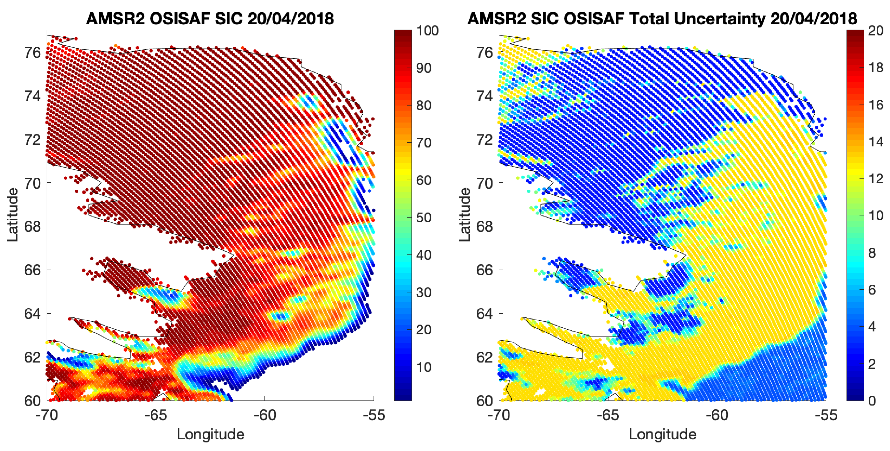
First, the methodology is applied to AMSR2 observations for one clear sky scene over the north polar region and compared to SIC estimates from visible/near-infrared Moderate Resolution Imaging Spectroradiometer (MODIS) imagery. The operational SIC product from the EUMETSAT Ocean Sea Ice—Satellite Application Facilities (OSI SAF, www.osi-saf.org), derived from AMSR2 observations, is also examined [8,13]. Second, evaluations are performed at large scales, over north and south polar regions, during both winter and summer.

Section 2 summarizes the methodology and presents the satellite observations and products. In Section 3, the results are assessed locally over a boreal region under clear sky conditions, whereas large scale results are discussed in Section 4. Section 5 concludes this study, insisting on the future potential developments.

2. Method and Materials

2.1. The IceCREAM Algorithm

This new methodology is particularly adapted for the CIMR mission. It follows the optimal estimation scheme that is often adopted for the retrieval of geophysical parameters from satellites [17]. It is very flexible and allows using different channel combinations to retrieve the SIC. The method requires a forward model that establishes the relationship between the SIC and the brightness temperatures (TBs) measured by the satellite. The forward model is empirically based on the contrast between ocean and ice TBs. The mean TBs for the open ocean (corresponding to 0% SIC) and for the total ice cover (corresponding to 100% SIC ) are estimated from the collection of passive microwave observations contained in the RRDP. Then, the forward model is simply a linear mixing model derived from the TB contribution of the two extreme surface types within the sensor footprint. With the optimal estimation scheme, a theoretical retrieval error is systematically attached to each inversion.

Tests have been performed using different combinations of channels between 6 and 36 GHz. The algorithm with the 6 and 10 GHz (both vertical and horizontal polarizations) is rather insensitive to changes in the sea ice environments, with a low theoretical retrieval error. However, these low frequency channels only provide low spatial resolution estimates. The algorithm using the 18 and 36 GHz (both vertical and horizontal polarizations) shows larger retrieval errors, but with an improved spatial resolution.

The CIMR mission will provide the same spatial resolution (15 km) for the 6 and 10 GHz channels, and the same spatial resolution (5 km) for the 18 and 36 GHz channels. The IceCREAM algorithm proposes a method to combine the SIC estimate at high resolution using the 18 and 36 GHz channels, with the low resolution estimation using the 6 and 10 GHz channels. The SIC estimate at low resolution is used to correct the SIC estimates at high resolution that are within the low resolution pixel, using a data fusion scheme.

More detail about the IceCREAM method is provided in Kilic et al. [15] (Part 1 of this study).

2.2. MODIS Sea Ice

MODIS instrument observes the Earth from visible to infrared wavelengths. With its polar orbit and large swath (∼2300 km), it frequently covers the polar regions. Under clear sky conditions, presence of sea ice can be detected from MODIS, using combination of thresholds on the observed reflectances in the visible and near-infrared bands. For comparison with the passive microwave SIC products, the sea ice day product from MODIS on board the Aqua mission (MYD29P1D) at 1 km spatial resolution is selected here, as provided by the National Snow and Ice Data Center (NSIDC) [18]. Each oceanic 1 km pixel is classified as ice, ocean, or cloud. A predominantly clear sky case over the north polar region is selected, on 4 April 2018, and the corresponding NSIDC MODIS sea ice product is downloaded. Figure 1 (left) presents the NSIDC MODIS sea ice product for the selected situation over the north polar region. The sea ice cover is showing large discontinuities in the Davis Strait, between the Baffin Island and Greenland. Although not visible at the resolution of the figure, the ice edges are often contaminated by clouds in the MODIS products. This is partly explained by cold winds blowing from sea ice to ocean and generating clouds at the contact with the ’warm’ ocean. It could also be partly related to algorithm problems in these transition zones. Other situations have been analyzed but are not shown here.

The MODIS sea ice product is spatially averaged over the AMSR2 footprints, to produce a MODIS-derived SIC estimate comparable with the AMSR2 SIC products. Figure 1 (right) presents the results at the 18 GHz spatial resolution for the selected image (18 km at this frequency, see Table 1). The MODIS SIC within an AMSR2 footprint is calculated as the ratio between the number of MODIS sea ice pixels versus the sum of sea ice pixels and ocean pixels, without counting the cloudy 1 km pixels. Different thresholds on the number of acceptable cloudy pixels within the AMSR2 footprint have been tested. If no cloudy pixels are tolerated, MODIS-derived SIC at AMSR2 resolution can seldom be calculated around the ice edges. On the contrary, if a very large fraction of clouds is accepted, the MODIS-derived SIC is meaningless. Several tests showed that a threshold of 50% on the cloud percentage in the AMSR2 footprint was providing acceptable results, even over the ice edges.

2.3. AMSR2

The AMSR2 instrument has already been briefly described (Table 1). The AMSR2 data are extracted from the JAXA data center (https://suzaku.eorc.jaxa.jp/GCOM_W/index.html). The level L1R product is used [19]. To mimic the fact that the CIMR instrument has the same spatial resolution at 6 and 10 GHz and at 18 and 36 GHz respectively, the 10 GHz observations are spatially averaged to the 6 GHz resolution, and the 36 GHz observations are averaged to the 18 GHz footprint, all provided by the L1R dataset. The observations are sampled at 12 km. Figure 2 shows the 6 and 36 GHz brightness temperature (TB) images at vertical polarization, for the selected situation. The 6 GHz observations are displayed at their nominal resolution and the 36 GHz observations at the 18 GHz resolution. As discussed in Part 1, among the selected frequencies, the 6 and 36 GHz frequencies have respectively the highest and the lowest sensitivity to the presence of ice. The spatial structures in Figure 2 are very similar to the sea ice extent derived from the MODIS images (see Figure 1), emphasizing the sensitivity of these observations to the presence of sea ice. Even directly on the TB maps, the discontinuities in the sea ice cover are observable. The different sensitivities to the sea ice at 6 and 36 GHz are obvious, with much more contrast between the ocean and sea ice TBs at 6 than at 36 GHz. More small structures are observed with the 36 GHz, especially at the sea ice edge, as expected from the better spatial resolution at this frequency. Note that at 6 GHz vertical polarization, continental ice has very similar signatures than the sea ice, at least close to the coasts in this region.

2.4. OSI SAF SIC

The AMSR2 sea ice concentration product of the OSI SAF (OSI-408) is compared to the IceCREAM estimates. The OSI SAF Hybrid Dynamic product is extracted for the selected situation, as well as for large scale comparisons for both north and south polar regions. The algorithm uses 18 and 36 GHz observations at vertical polarization. It is a combination of the NASA Bootstrap algorithm [11,20] for low SIC and the Bristol algorithm [12] for high SIC. It includes water vapor correction over the ocean, using Numerical Weather Prediction analysis and a radiative transfer model. To account for their time variations, the algorithm anchor points (also called the tie points) for pure sea ice and open ocean are regularly updated. Filters and masks are further applied to avoid algorithm artifacts (along coast lines for instance). The product is available on a 10 km polar stereographic grid. An uncertainty assessment is attached to each SIC estimate: it includes the intrinsic algorithm uncertainty and the so-called smearing uncertainty due to the sampling of different frequency footprints onto a single grid. For a full description of the dynamic hybrid algorithm and the derived dataset, see [8,13].

For the selected scene, the OSI SAF SIC is presented in Figure 3, along with its total uncertainty (the sum of the algorithm and smearing uncertainties). The spatial structures of the OSI SAF SIC are in very good agreement with the SIC estimates from MODIS (Figure 1). Note that the total uncertainty is dominated by the smearing uncertainty, with a maximum of ∼5% in the algorithm uncertainty (not shown).

3. Results and Discussion for a Local Scene

For the selected situation, the SIC estimates are tested with different algorithm choices. First, the frequency selection is assessed. Second, the impact of the tie points is evaluated, and finally, the fusion of the low and high resolution results is examined. Note that other local scenes have been studied with similar results.

3.1. Frequency Selection and Sensitivity to the Tie Points

First, the inversion algorithm is applied to the combination of the 6 and 10 GHz channels and the 18 and 36 GHz channels, respectively, using both perpendicular polarizations for all considered frequencies (named 6+10GHz and 18+36GHz algorithms in the following). The RRDP [9] is a database of satellite observations at 0% and 100% SIC (see Part 1 for more information on its use here). The full RRDP is used to derive the sensitivity of the observations to the SIC (north and south polar regions, for all seasons). The algorithm theoretical error standard deviations (stds) are also systematically calculated, as described in Part 1. As already mentioned, the observations are considered at the spatial resolution of the lower frequency channel used in the algorithm (i.e., for the 18+36GHz combination, the 36 GHz observations are averaged on the 18 GHz spatial resolution and for the 6+10GHz combination, the 10 GHz observations are averaged on the 6 GHz spatial resolution). Note that in current SIC operational algorithms (OSI SAF for instance), each observation is used at its original resolution and the spatial resolution issue is accounted for by an additional term in the error budget (the smearing error) [13].

Figure 4 presents the results of the retrievals, along with the algorithm theoretical error StDs. The results of our 18+36GHz algorithm appear very similar to the OSI SAF results (Figure 3) (despite their different projections: our results are provided at the swath level whereas the OSI SAF results are gridded on a 10 km polar stereographic grid). It is also clear that the 18+36GHz algorithm provides better spatial resolution than the 6+10GHz combination, with very blurred structures for the 6 +10 GHz combination. However, the associated theoretical error std is significantly better for the 6+10GHz algorithm than for the high frequency one, as expected.

To better quantify the differences between the retrievals, the histograms of the SIC distributions are provided in Figure 5, for the MODIS estimates at the spatial resolution of the AMSR2 18 GHz, for the 6+10GHz and 18+36GHz retrievals we developed using the full RRDP (solid lines). The pixels that are cloud contaminated at more than 50% are excluded for the comparisons, as estimated by MODIS. The MODIS estimates show very large populations at 0% and 100%, and a limited population with partial ice cover. This is partly related to the fact that the sea ice edges are often cloudy, but also likely to some ambiguities in the detection of sea ice edges and clouds with MODIS as already mentioned. AMSR2 estimates have broader peaks, especially around 100% for the 18+36GHz algorithms. The maxima of these peaks are not at 0 or 100%, with some pixels below 0% and a significant population of pixels above 100% for the 18+36GHz algorithm. This is in agreement with the results from Part 1 that showed that the 18+36GHz algorithms have larger systematic and random errors than the 6+10GHz combinations. Note nevertheless that the peaks of the 6+10GHz distribution are not strictly at 100% and 0% as expected, but rather are shifted slightly below 100% and slightly above 0%: the 6+10GHz algorithm is expected to provide unbiased results at a global scale, averaged over a full seasonal cycle, as described by the full RRDP (see Part 1). Here, only one scene is presented, for the north polar region at a given time in the year, and some bias is observed as the responses of the 6 and 10 GHz to the sea and ice conditions in this specific situation do not perfectly match the averaged conditions in the RRDP.

Changes in the tie points (dynamic tie points) have been applied in operational method such as the OSI SAF algorithm, to account for the impact of the sea ice variability on the microwave observations as a function of location and season. Here, the effect of modifying the tie points is tested in our algorithm by selecting only part of the full RRDP to derive the sensitivity of the observations to the SIC. Only the situations collected over the north polar region are selected, first for the winter months, then for the summer months. The histograms of the SIC results for the same scene are presented in Figure 5 (dashed lines), as compared to the results using the full RRDP (solid lines). Some changes are observed in the SIC distributions, both for the 6+10GHz and 18+36GHz algorithms, but they are limited, confirming the results obtained in Part 1. From now on, the sensitivity of the observations will be derived from the full RRDP (both polar regions, all seasons).

Under this clear sky situation, the 6+10GHz algorithm already shows lower errors than the 18+36GHz combination. It is expected that the low frequency algorithm would even be more beneficial for cloudy scenes, as clouds mostly affect the high frequencies.

3.2. Fusion of the Retrievals at Low and High Resolutions

There is a ratio of 3 in the spatial resolutions of the 6 and 18 GHz for both AMSR2 and CIMR instruments. The CIMR instrument is designed to have the same ∼15 km spatial resolution at 6 and 10 GHz, and the same ∼5 km spatial resolution at 18 and 36 GHz, to facilitate the combination of the low and high frequency channels, respectively. Here, we test the methodology described in Part 1 to combine the large sensitivity of the 6+10GHz algorithm to the SIC with the high spatial resolution of the 18+36GHz retrieval.

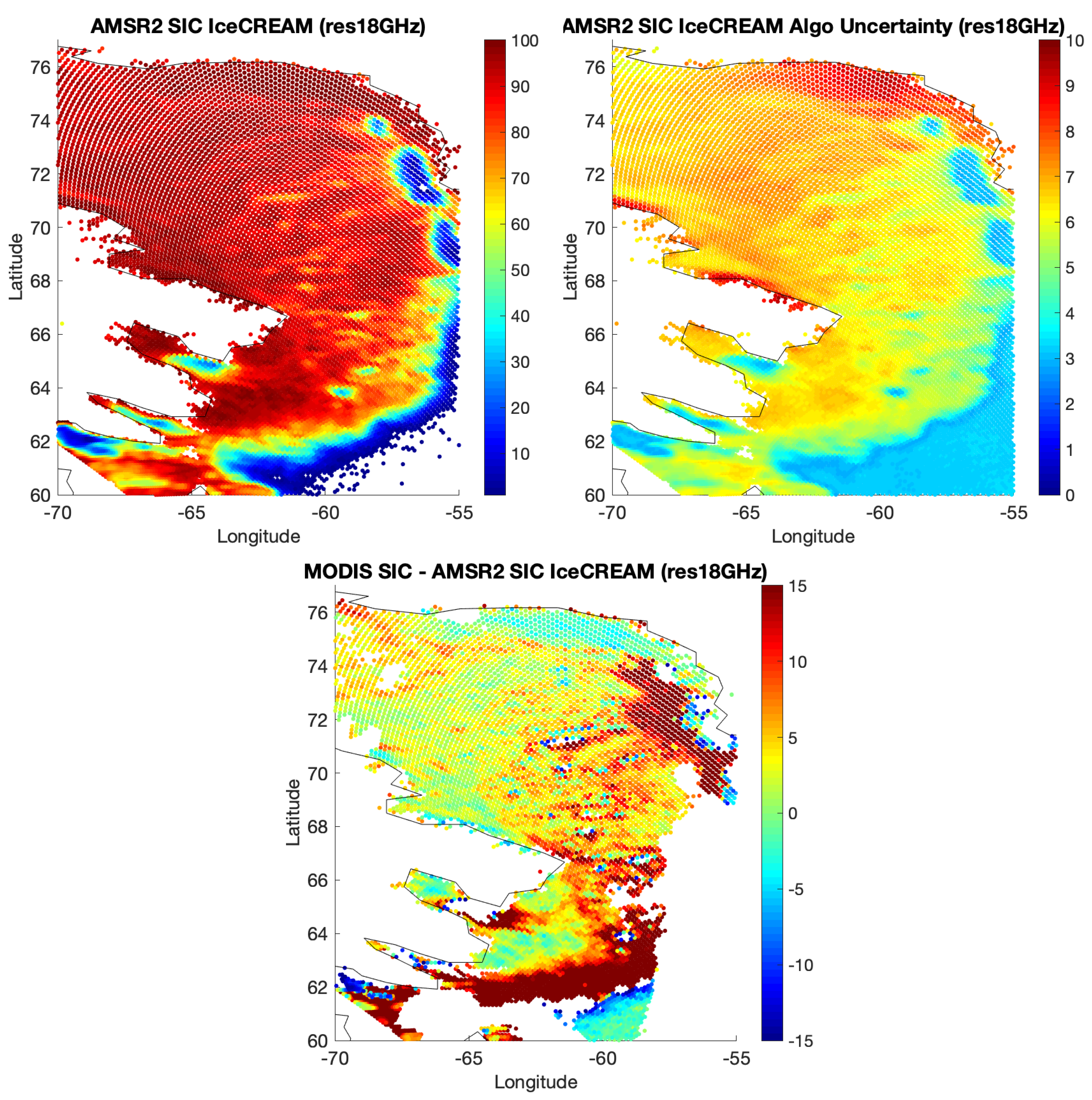
The IceCREAM methodology consists in performing the retrieval separately for the lower frequencies (6+10GHz) and the higher frequencies (18+36GHz) first, and then in using the low frequency retrieval to de-bias all the high frequency retrievals that fall within the low frequency/low spatial resolution retrieval. The lower frequency retrieval provides good accuracy and precision but with low spatial resolution. On the contrary, the high frequency retrieval has good spatial resolution, but with large errors. The solution consists in averaging each individual high spatial resolution retrieval within a low resolution pixel, to fit the low resolution retrieval. The averaging takes into account the respective uncertainty of the individual high spatial resolution retrieval. This can be seen as a disaggregation of the low frequency retrieval, using the high frequency retrieval at high spatial resolution. This solution is particularly well suited for CIMR, as the low frequency channels at 6 and 10 GHz (respectively high frequency channels at 18 and 36 GHz) will have very similar spatial resolutions, i.e., their combination (6 and 10 GHz on one side and 18 and 36 GHz on the other side) will not raise any spatial resolution issue, providing a final product at the high spatial resolution. For the same local scene, the previous results of the 18+36GHz retrieval are tuned to match the coinciding results at 6+10GHz, taking into account the respective errors of the results, following the method developed in Part 1. The map of the SIC results is presented in Figure 6, along with the corresponding error std. For the same scene, Figure 6 also shows the difference between the MODIS SIC (as calculated from spatial averaging over the 18 GHz AMSR2 footprint, when the cloud cover is less than 50%) and the IceCREAM SIC results. Over regions of high (close to 100%) and low (close to 0%) SIC, limited differences are observed between MODIS and IceCREAM SIC. However, in regions of intermediate SIC (see for instance the large differences around 62${}^{\circ }$N or around −57${}^{\circ }$E), the differences are significant. This can be related to the use of the linear forward model in the retrieval that implicitly assumes that the microwave response to the sea ice is the same regardless of the ice nature between 0% and 100% SIC. Around the ice margin, the ice physical characteristics are likely different, with impact on the ice microwave responses, leading to errors in the microwave SIC. In addition, as already mentioned, the MODIS SIC estimates also show limitations in the ice margin areas, with ambiguities with cloud cover.

For a more detailed assessment of the results, the histograms of the resulting SIC distribution is shown, compared to the MODIS estimates at 18 GHz resolution and the 6+10GHz and 18+36GHz algorithms (Figure 7). The distribution of the results for the fusion of the 6+10GHz and 18+36GHz algorithms (the all channel results) is close to the results at 6+10GHz, with low bias and a limited dispersion around the maximum, especially close to 100% SIC. 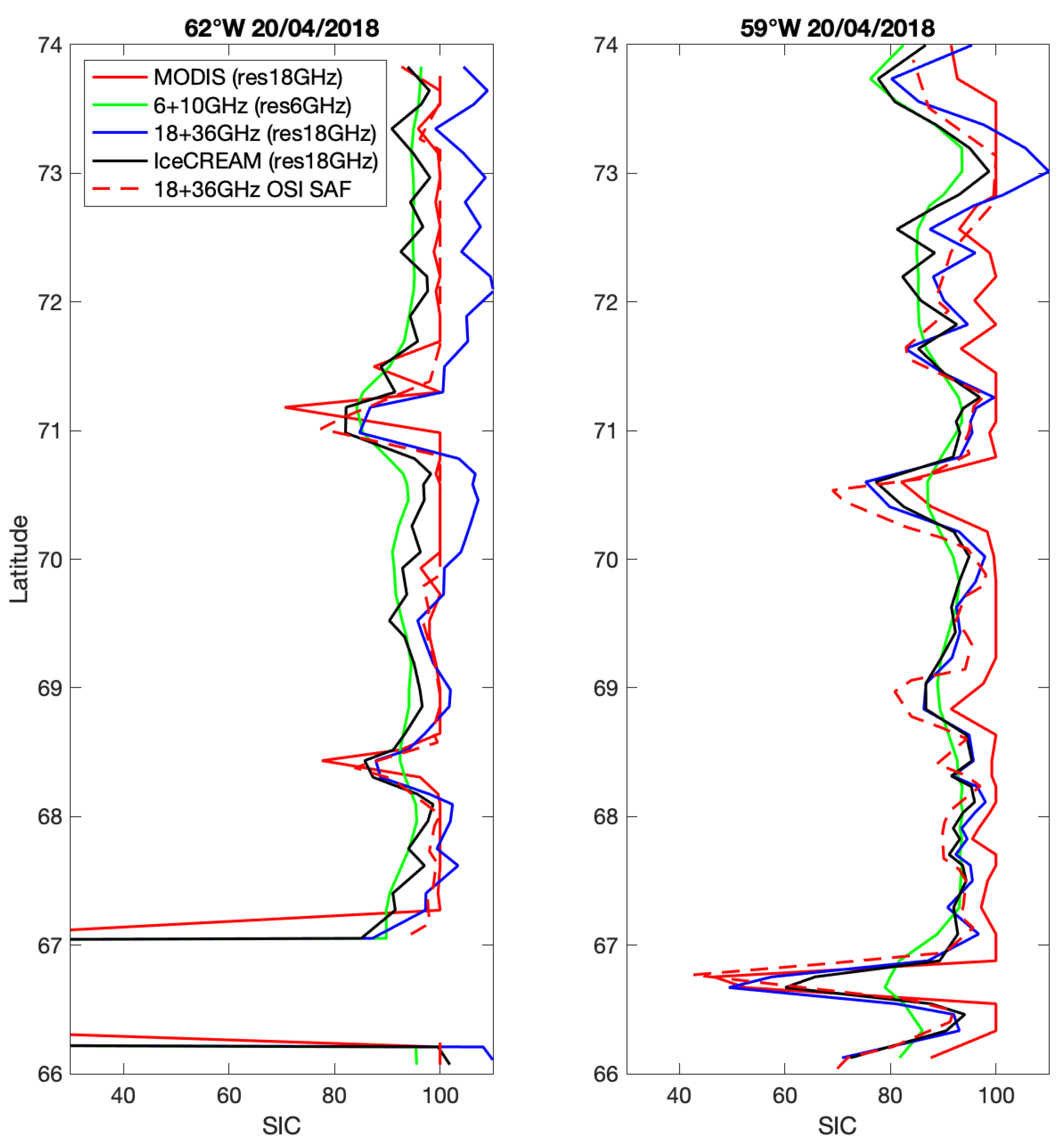In addition, Figure 8 presents a comparison of the SIC estimates over two transects for the scene, at 62${}^{\circ }$W and 59${}^{\circ }$W. The following products are evaluated: the MODIS estimates at 18 GHz resolution, our AMSR2 6+10GHz and 18+36GHz retrievals, our retrieval combining all the frequencies (fusion of the 6+10GHz and 18+36GHz retrievals), and the OSI SAF operational products.

All the AMSR2-derived SIC retrievals follow reasonably well the MODIS estimates. Our SIC estimates with the 18+36GHz algorithm are in good agreement with the OSI SAF operational product (also derived from the same frequencies), although we do not apply any tie point changes nor any weather filtering on our results. We deliberately do not adopt a threshold at 0% and 100% on our SIC, to illustrate the uncertainties related to our 18+36GHz algorithm: in operational mode, thresholds would obviously be applied. With the 6+10GHz algorithm, the spatial structures are clearly smeared, as compared to the other products with higher spatial resolution. Combining all the frequencies provides results that show the spatial resolution of the 18+36GHz combination, but with values closer to the 6+10GHz algorithm that has been shown to have less systematic and random errors.

4. Results and Discussion at Large Scales Over the Polar Regions

The method is tested at large scales over the north and south polar regions, for both winter and summer. The previous case study was limited to clear sky conditions, for comparison with MODIS data. It focussed on the Arctic at the end of the winter. Here, both clear and cloudy situations are considered, for two seasons, and for both polar regions. The same collection of observations from the full RRDP is used to estimate the sensitivity of the microwave observations to the SIC, for both hemispheres and seasons.

Two days are selected, 30 January 2018, and 30 August 2018. The following estimates are compared: our 6+10GHz and 18+36GHz algorithms, the combination of these two results (the all channel IceCREAM results), and the original OSI SAF estimates. Figure 9 and Figure 10 present the results for the north and south polar regions respectively, for the selected days in January and August. On Figure 9 and Figure 10, the SIC values lower than 5% have been systematically omitted, for all estimates, including for the OSI SAF results. No other filtering has been applied to our estimates (no coastal or atmospheric filtering).

Figure 9 and Figure 10 show that the SIC spatial structures are globally very similar for all algorithms, with the 6+10GHz results having the coarser spatial resolution, as expected. Our results do not show obvious errors that would be related to the use of a unique set of tie points, regardless of the polar region and the season. Some unrealistic SICs are observed with the 18+36GHz algorithm, in regions that are very likely ice-free (especially over the north polar region in August). If this algorithm was applied operationally, post filtering would be necessary. Combining all the frequencies with the IceCREAM scheme makes it possible to suppress the noisy signals of the 18+36GHz while benefiting from the high spatial resolution at these frequencies.

On August 30, the cloud cover was particularly dense over the Arctic high latitudes, especially south west of Greenland, likely associated with precipitation in some locations. This was confirmed with the help of the NASA viewing tool, https://worldview.earthdata.nasa.gov. The OSI SAF product erroneously detects a sea ice zone in the region of very thick clouds on that day (Figure 9, top right panel). We checked that the day before and the day after this structure was not present on the OSI SAF products. The algorithm based on the 18 and 36 GHz vertical polarizations is contaminated by the presence of clouds. Our 18+36GHz algorithm that uses both polarizations for the two frequencies is not seriously affected, and once combined with the 6+10GHz, it is clearly more robust to cloud contamination.

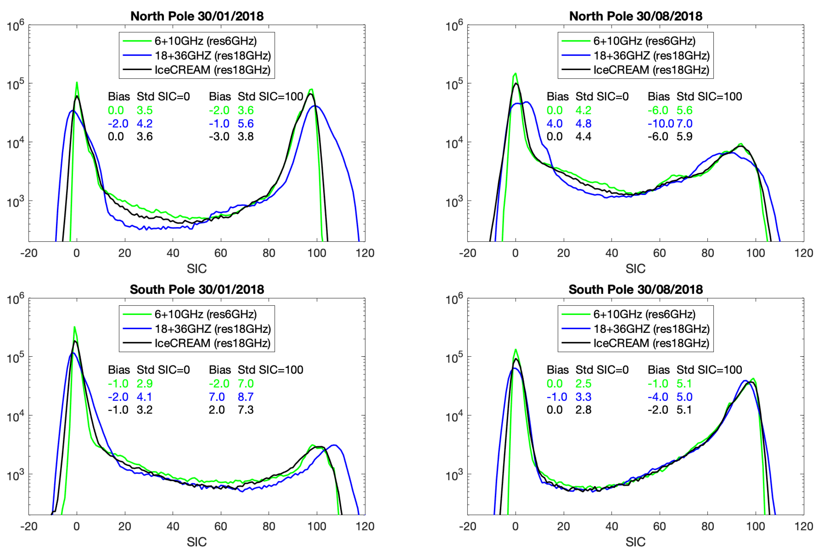
For the same two days and for both polar regions, the SIC distributions for the three retrievals (6+10GHz, 18+36GHz, and IceCREAM) are presented in Figure 11. Over these large regions, we expect a maximum of the SIC distribution at 0% and at 100%, and the departures of peak values in the distributions can be considered as biases. These biases have been systematically calculated for the four situations and for the three algorithms, along with the corresponding standard deviations (stds) around these biases, and are added on Figure 11. For all the algorithms, the performances are better at 0% (lower bias and std) than at 100% SIC. In addition, the performances tend to be lower during summer than during winter in the same region, especially for the 100% SIC. This is directly related to the melting conditions in summer, where the microwave signatures over ice can show larger variabilities than during winter. The 6+10GHz retrieval has almost always the best performances, at 0% and at 100% SIC, both in terms of bias and standard deviation. On the contrarily, the 18+36GHz algorithm has often the worse performances. Of course, in terms of spatial resolution, the 18+36GHz retrieval clearly defeats the 6+10GHz algorithm. With the same spatial resolution as the 18+36GHz algorithm, the performances obtained with IceCREAM are improved with respect to the 18+36GHz ones, and close to the 6+10GHz ones. IceCREAM successfully combines the low errors of the low frequency algorithm, with the high spatial resolution of the high frequency retrieval.

5. Conclusions

A simple and flexible retrieval framework has been developed to estimate the SIC from passive microwave satellite observations between 6 and 36 GHz. It is based on the use of a collection of satellite observations at 0% and 100% SIC (the RRDP).

Different frequency combinations can be used, to minimize the uncertainty or to maximize the spatial resolution of the products. A solution is proposed here to optimize both, using all the frequency range from 6 to 36 GHz. It is a two step algorithm. First, the SIC is estimated at the low spatial resolution of the 6 GHz, using 6 and 10 GHz observations (both polarizations), and at the high spatial resolution of the 18 GHz, using the 18 and the 36 GHz (both polarizations). Second, the high spatial resolution 18+36GHz results within a low resolution 6+10GHz pixel are bias-corrected to match the 6+10GHz result, taking into account the respective errors of the products. This is the IceCREAM algorithm.

The algorithm is tested with AMSR2 observations, for a clear sky local scene with collocated MODIS estimates. It is also tested for the full polar regions, winter and summer, under clear and cloudy conditions. The OSI SAF operational product is also compared with our methodology. Our SIC results are very encouraging, providing both low errors related to the low frequency observations and high spatial resolution obtained from the high frequencies.

The method is developed for the CIMR project. It is evaluated here with AMSR2 observations. Better performances are expected with CIMR. First the spatial resolution of the instrument will be largely improved for all channels. Second, the 6 and 10 GHz (resp. the 18 and 36 GHz) will have the same resolution at ∼15 km (resp. at ∼5 km), making it natural to first exploite the collocated 6 and 10 GHz (resp. 18 and 18 GHz) observations before combining them.

Further refinements are expected in the near future, with the use of a radiative transfer model for the open ocean, to replace the RRDP information for the 0% SIC situations. Development of an updated open ocean microwave emissivity model is underway. It builds upon recent work [21] showing that the current sea surface emissivity models still have difficulties under high wind speed conditions and in cold regions. It will reduce the uncertainty in the open ocean signature and it will duly account for the atmospheric contribution, using information from coincident Numerical Weather Prediction analyses. Once these improvements are implemented, the IceCREAM algorithm will be applied to the AMSR-E and AMSR2 collections over both polar regions.

References

1. Simmonds, I. Comparing and contrasting the behaviour of Arctic and Antarctic sea ice over the 35 year period 1979-2013. Ann. Glaciol. 2015, 56, 18–28. [Google Scholar] [CrossRef] [Green Version]
2. Notz, D.; Stroeve, J. Observed Arctic sea-ice loss directly follows anthropogenic CO2 emission. Science 2016, 354, 747–750. [Google Scholar] [CrossRef] [PubMed] [Green Version]
3. Screen, J.A.; Simmonds, I. The central role of diminishing sea ice in recent Arctic temperature amplification. Nature 2010, 464, 1334–1337. [Google Scholar] [CrossRef] [PubMed] [Green Version]
4. Dai, A.; Luo, D.; Song, M.; Liu, J. Arctic amplification is caused by sea-ice loss under increasing CO2. Nat. Commun. 2019, 10, 1–13. [Google Scholar] [CrossRef] [PubMed] [Green Version]
5. Screen, J.A.; Simmonds, I. Exploring links between Arctic amplification and mid-latitude weather. Geophys. Res. Lett. 2013, 40, 959–964. [Google Scholar] [CrossRef] [Green Version]
6. Mori, M.; Watanabe, M.; Shiogama, H.; Inoue, J.; Kimoto, M. Robust Arctic sea-ice influence on the frequent Eurasian cold winters in past decades. Nat. Geosci. 2014, 7, 869. [Google Scholar] [CrossRef]
7. Luo, B.; Wu, L.; Luo, D.; Dai, A.; Simmonds, I. The winter midlatitude-Arctic interaction: Effects of North Atlantic SST and high-latitude blocking on Arctic sea ice and Eurasian cooling. Clim. Dyn. 2019, 52, 2981–3004. [Google Scholar] [CrossRef]
8. Tonboe, R.T.; Eastwood, S.; Lavergne, T.; Sørensen, A.M.; Rathmann, N.; Dybkjær, G.; Pedersen, L.T.; Høyer, J.L.; Kern, S. The EUMETSAT sea ice concentration climate data record. Cryosphere 2016, 10, 2275–2290. [Google Scholar] [CrossRef] [Green Version]
9. Pedersen, L.T.; Saldo, R. Sea Ice Concentration (SIC) round robin data package. In Sea Ice Climate Change Initiative; Technical Report; ESA: Noordwijk, The Netherlands, 2017. [Google Scholar]
10. Cavalieri, D.J.; Gloersen, P.; Campbell, W.J. Determination of sea ice parameters with the Nimbus 7 SMMR. J. Geophys. Res. Atmos. 1984, 89, 5355–5369. [Google Scholar] [CrossRef]
11. Comiso, J.; Sullivan, C. Satellite microwave and in situ observations of the Weddell Sea ice cover and its marginal ice zone. J. Geophys. Res. Ocean. 1986, 91, 9663–9681. [Google Scholar] [CrossRef]
12. Smith, D. Extraction of winter total sea-ice concentration in the Greenland and Barents Seas from SSM/I data. Remote Sens. 1996, 17, 2625–2646. [Google Scholar] [CrossRef]
13. Lavergne, T.; Sørensen, A.M.; Kern, S.; Tonboe, R.; Notz, D.; Aaboe, S.; Bell, L.; Dybkjær, G.; Eastwood, S.; Gabarro, C.; et al. Version 2 of the EUMETSAT OSI SAF and ESA CCI sea-ice concentration climate data records. Cryosphere 2019, 13, 49–78. [Google Scholar] [CrossRef] [Green Version]
14. Ivanova, N.; Pedersen, L.T.; Tonboe, R.T.; Kern, S.; Heygster, G.; Lavergne, T.; Sørensen, A.; Saldo, R.; Dybkjær, G.; Brucker, L.; et al. Inter-comparison and evaluation of sea ice algorithms: Towards further identification of challenges and optimal approach using passive microwave observations. Cryosphere 2015, 9, 1797–1817. [Google Scholar] [CrossRef] [Green Version]
15. Kilic, L.; Prigent, C.; Aires, F.; Heygster, G.; Pellet, V.; Jimenez, C. Ice Concentration Retrieval from the Analysis of Microwaves: A New Methodology Designed for the Copernicus Imaging Microwave Radiometer. Remote Sens. 2020, 12, 1060. [Google Scholar] [CrossRef] [Green Version]
16. Kilic, L.; Prigent, C.; Aires, F.; Boutin, J.; Heygster, G.; Tonboe, R.T.; Roquet, H.; Jimenez, C.; Donlon, C. Expected Performances of the Copernicus Imaging Microwave Radiometer (CIMR) for an All-Weather and High Spatial Resolution Estimation of Ocean and Sea Ice Parameters. J. Geophys. Res. Ocean. 2018, 123, 7564–7580. [Google Scholar] [CrossRef] [Green Version]
17. Rodgers, C.D. Inverse Methods for Atmospheric Sounding: Theory and Practice; World Scientific: Singapore, 2000; Volume 2. [Google Scholar]
18. Hall, D.K.; Riggs, G.A. MODIS/Aqua Sea Ice Extent 5-Min L2 Swath 1 km, Version 6; NASA National Snow and Ice Data Center Distributed Active Archive Center: Boulder, CO, USA, 2015; 10.
19. Maeda, T.; Taniguchi, Y.; Imaoka, K. GCOM-W1 AMSR2 level 1R product: Dataset of brightness temperature modified using the antenna pattern matching technique. IEEE Trans. Geosci. Remote Sens. 2016, 54, 770–782. [Google Scholar] [CrossRef]
20. Comiso, J.; Cavalieri, D.J.; Parkinson, C.L.; Gloersen, P. Passive microwave algorithms for sea ice concentration: A comparison of two techniques. Remote Sens. Environ. 1997, 60, 357–384. [Google Scholar] [CrossRef]
21. Kilic, L.; Prigent, C.; Boutin, J.; Meissner, T.; English, S.; Yueh, S. Comparisons of Ocean Radiative Transfer Models With SMAP and AMSR2 Observations. J. Geophys. Res. Ocean. 2019, 124, 7683–7699. [Google Scholar] [CrossRef]
Figure 1. The Moderate Resolution Imaging Spectroradiometer (MODIS) sea ice information for the selected scene, 20 April 2018. Left: the original MODIS sea ice data at 1 km spatial resolution. Right: the MODIS-derived Sea Ice Concentration (SIC), as calculated from spatial averaging over the 18 GHz AMSR2 footprint, when the cloud cover is less than 50%. The landmasses are Greenland in the north-east of the image and Baffin Island in the west.
Remotesensing 12 01594 g001
Figure 2. The AMSR2 data for the selected scene, 20 April 2018. Left: the 6 GHz vertical polarization (at its nominal spatial resolution). Right: the 36 GHz vertical polarization (at the 18 GHz spatial resolution).
Remotesensing 12 01594 g002
Figure 3. The Ocean Sea Ice—Satellite Application Facilities (OSI SAF) results for the selected scene, 20 April 2018. Left: the sea ice concentration (SIC). Right: the total uncertainty on that product (the sum of the algorithm and smearing uncertainties).
Remotesensing 12 01594 g003
Figure 4. SIC retrieval results for the 20 April 2018 scene, along with the corresponding algorithm theoretical error std. Left: for the 6+10GHz combination (the SIC on the top and the corresponding error on the bottom). Right: same for the 18+36GHz combination.
Remotesensing 12 01594 g004
Figure 5. For the 20 April 2018 scene, the histograms of the SIC for MODIS at 18 GHz resolution in red, for our algorithms using the full RRDP with 6+10GHz in green (solid line), and for 18+36GHz in blue (solid line). Comparisons of our 6+10GHz and 18+36GHz AMSR2 algorithms using different subsets of the RRDP are also presented: limited to the north polar region for the winter season (dash lines) and then limited to the north polar region for the summer season (dash-dotted lines). The pixels that are cloud contaminated at more than 50% are excluded, as estimated by MODIS.
Remotesensing 12 01594 g005
Figure 6. Top left: IceCREAM SIC retrieval results for the 20 April 2018 scene, when combining all the channels, i.e., the low (6+10GHz) and the high (18+36GHz) frequency algorithms. Top right: the corresponding theoretical retrieval error std. Bottom: Difference between the MODIS SIC and the IceCREAM SIC results. The MODIS SIC is calculated from spatial averaging over the 18 GHz AMSR2 footprint, when the cloud cover is less than 50% (leading to holes in the image).
Remotesensing 12 01594 g006
Figure 7. For the 20 April 2018 scene, the histograms of the SIC for MODIS at 18 GHz resolution in red, for our 6+10GHz AMSR2 algorithm in green, for our 18+36GHz AMSR2 algorithm in blue, and for the IceCREAM retrieval (all channel algorithm in black). The pixels that are cloud contaminated at more than 50% are excluded, as estimated by MODIS.
Remotesensing 12 01594 g007
Figure 8. Transects over the scene, for different SIC estimates. Left: at 62 W. Right: at 59 W. The following products are compared: the MODIS estimates at 18 GHz resolution, our AMSR2 retrieval at 6+10GHz (at the spatial resolution of the 6 GHz) and at 18+36GHz (at the spatial resolution of the 18 GHz), the combination of these two results (the IceCREAM all channel results at the spatial resolution of the 18 GHz), and the OSI SAF operational products.
Remotesensing 12 01594 g008
Figure 9. Over the north polar region, from left to right, comparison of our 6+10GHz and 18+36GHz algorithms, the all channel IceCREAM results, and the original OSI SAF estimates (using 18 and 36 GHz V polarization). Top: 30 January, 2028. Bottom: 30 August, 2018. Note that the values of SIC below 5% have been suppressed for all the estimates.
Remotesensing 12 01594 g009
Figure 10. Same as Figure 9, over the south polar region.
Remotesensing 12 01594 g010
Figure 11. Histograms of our SIC estimates, for the north (top) and the south (bottom) polar regions, for 30 January 2018 (left), and for 30 August 2018 (right), for the 6+10GHz, the 18+36GHz, and the IceCREAM algorithms. A logarithmic scale is used for the y-axis. For SIC at 0% and SIC at 100%, the bias and the std are indicated for each algorithm, with the same color code. See the text for more detail.
Remotesensing 12 01594 g011