Field Intercomparison of Radiometer Measurements for Ocean Colour Validation

Abstract

A field intercomparison was conducted at the Acqua Alta Oceanographic Tower (AAOT) in the northern Adriatic Sea, from 9 to 19 July 2018 to assess differences in the accuracy of in- and above-water radiometer measurements used for the validation of ocean colour products. Ten measurement systems were compared. Prior to the intercomparison, the absolute radiometric calibration of all sensors was carried out using the same standards and methods at the same reference laboratory. Measurements were performed under clear sky conditions, relatively low sun zenith angles, moderately low sea state and on the same deployment platform and frame (except in-water systems). The weighted average of five above-water measurements was used as baseline reference for comparisons. For downwelling irradiance ($E_d$), there was generally good agreement between sensors with differences of <6% for most of the sensors over the spectral range 400 nm–665 nm. One sensor exhibited a systematic bias, of up to 11%, due to poor cosine response. For sky radiance ($L_{sky}$) the spectrally averaged difference between optical systems was <2.5% with a root mean square error (RMS) <0.01 mWm⁻² nm⁻¹ sr⁻¹. For total above-water upwelling radiance ($L_t$), the difference was <3.5% with an RMS <0.009 mWm⁻² nm⁻¹ sr⁻¹. For remote-sensing reflectance ($R_{rs}$), the differences between above-water TriOS RAMSES were <3.5% and <2.5% at 443 and 560 nm, respectively, and were <7.5% for some systems at 665 nm. Seabird-Hyperspectral Surface Acquisition System (HyperSAS) sensors were on average within 3.5% at 443 nm, 1% at 560 nm, and 3% at 665 nm. The differences between the weighted mean of the above-water and in-water systems was <15.8% across visible bands. A sensitivity analysis showed that $E_d$ accounted for the largest fraction of the variance in $R_{rs}$, which suggests that minimizing the errors arising from this measurement is the most important variable in reducing the inter-group differences in $R_{rs}$. The differences may also be due, in part, to using five of the above-water systems as a reference. To avoid this, in situ normalized water-leaving radiance ($L_{wn}$) was therefore compared to AERONET-OC SeaPRiSM $L_{wn}$ as an alternative reference measurement. For the TriOS-RAMSES and Seabird-HyperSAS sensors the differences were similar across the visible spectra with 4.7% and 4.9%, respectively. The difference between SeaPRiSM $L_{wn}$ and two in-water systems at blue, green and red bands was 11.8%. This was partly due to temporal and spatial differences in sampling between the in-water and above-water systems and possibly due to uncertainties in instrument self-shading for one of the in-water measurements.

1. Introduction

Fiducial reference measurements (FRM) are an important component of satellite missions for the validation of remote sensing products and are used to ensure that the most accurate data are distributed to the user community. FRMs are distinct from other in situ measurements in that they use protocols recommended by international ocean colour organizations and space agencies, are traceable to SI (Système international) units, are referenced to inter-comparison exercises and have a full uncertainty budget [1] to provide independent, high quality validation measurements for the duration of a satellite mission [2,3]. To underpin the validation of satellite ocean colour radiometry, it is therefore essential that radiometers used to collect FRMs are inter-compared to assess data consistency and characterise the potential differences between instruments and methods. In the absence of such intercomparisons, the traceability chain and uncertainty budget are not validated. The use of a wide range of instruments, methods and laboratory practices may only add to the uncertainty of satellite ocean colour products.

The primary data product in satellite ocean colour is remote-sensing reflectance, $R_{rs}$. Radiometric field measurements used to derive this parameter are generally obtained from in-water and above-water optical measurements. These include above-water radiometry, underwater profiling, underwater measurements at fixed depths or combined above and underwater measurements from floating systems. Within the numerous measurement systems that exist, differences in calibration sources, methods and data processing schemes lead to the greatest variation between them [1,4]. To minimise these, best practices on each of the steps used to generate radiometric FRM have been established previously and in this project [5,6,7,8].

Since the launch of the Sea-Viewing Wide Field-of-View Sensor (SeaWiFS) in 1997, a growing body of literature on intercomparisons between radiometers has developed, which were conducted to constrain the differences between in-water and satellite ocean colour parameters [9,10,11,12,13,14,15,16,17]. The National Aeronautics and Space Administration (NASA) SeaWiFS Intercalibration Round Robin Experiments (SIRREX) 1–8 focused on sensor calibration; specifically spectral radiance response using plaques and portable field sources for monitoring the stability of sensors [9,10,11,12,13,14,15]. The experiments established protocols for these, which reduced the uncertainties in measurements from 8% to 1%. During SIRREX 5, comparisons between in-water radiometers were conducted at Little Seneca Lake in Maryland, USA and comparisons of above-water radiometers were conducted in the laboratory [11]. Differences in in-water apparent optical properties were found to be related to the stability of the platform and illumination geometry. For the laboratory comparisons, systematic differences between radiometers were associated with the derivation of the downwelling irradiance from the reflected plaque radiance and smaller differences due to isolated problems with the radiometers. These were addressed in SIRREX 8 through the publication of new laboratory methods for characterising irradiance sensors [15]. Then followed the NASA Sensor Intercomparison and Merger for Biological and Interdisciplinary Studies (SIMBIOS) Radiometric Intercomparison (SIMRIC) -1 and -2 [12,13]. The purpose of these experiments was to establish a common radiometric scale among the facilities that calibrate in situ radiometers used for ocean colour related research. The final result was an updated document on calibration procedures and protocols [9]. Using these protocols during SIMRIC-2, the SeaWiFS Transfer Radiometer (SXR-II) measured the calibration radiances at six wavelengths from 411 nm to 777 nm, which was compared against measurements from 10 other laboratories [13]. The agreement between laboratories was within the combined uncertainties for all but two laboratories and the errors for these laboratories were traced back to the sensor calibrations. Following the launch of the Medium Resolution Imaging Spectrometer (MERIS) in 2002, the MERIS and Advanced Along-Track Scanning Radiometer (AATSR) Validation Team (MAVT) conducted a series of intercomparison exercises (PlymCal 1-3 [14]) to compare above- and in- water radiometry (Bio-spherical, PR650, SATLANTIC, SIMBADA, SPMR, TACCS and TRIOS). The expected calibration of radiometric sensors is that they are within ±1 to 2% of each other and during these intercomparisons this was achieved, except for one sensor that exhibited degradation of the cosine collector. The MERIS Validation Team (MVT) then conducted a field campaign at a coastal site off South West Portugal and determined the accuracy of atmospheric and in-water measurements using a hyperspectral, SATLANTIC buoy radiometer with a tethered irradiance chain (TACCS), as well as band-pass filter radiometer of the same design [15]. The overall error for the TACCS system in these waters was 5% where the in-water attenuation coefficient ($K_d$) was known and 7% where $K_d$ was modelled and extrapolated from the surface to depth. Under the Assessment of In Situ Radiometric Capabilities for Coastal Water Remote Sensing Applications (ARC) MERIS MVT intercomparison of above-water radiometers (SeaPRISM and RAMSES) and in-water radiometers (WiSPER-Wire-Stabilized Profiling Environmental Radiometer and TACCS) was performed under near ideal deployment conditions at the Acqua Alta Oceanographic Tower (AAOT) in the northern Adriatic Sea [17]. For this intercomparison, all sensors were inter-calibrated through absolute radiometric calibration with the same standards and methods. The spectral water-leaving radiance ($L_w$), as well as $E_d$ and $R_{rs}$ were compared. The relative difference in $R_{rs}$ was between −1% and +6%. The spectrally averaged values of absolute difference were 6% for the above-water systems and 9% for the in-water systems. The good agreement between sensors was achievable because of the stability of the deployment platform used. The first in situ radiometer intercomparison exercise in support of the Ocean and Land Colour Instrument (OLCI) on-board the Sentinel-3 satellite was conducted at a lake in Estonia in May 2017 under non-homogeneous environmental conditions [4]. It highlighted that there was a large variability between recently calibrated sensors, due to high spectral and spatial variability in the targets and environmental conditions. For the radiance sensors tested, variation in the fields of view (FOV) contributed to the differences whereas for the irradiance sensors, this arose from imperfect cosine response. Following the success of ARC MERIS MVT, and because the environmental conditions are nearly ideal during summer, the AAOT was chosen to undertake the intercomparison reported here. The main difference over the previous intercomparisons at the AAOT was that: (1) more measurement systems were compared (10 in this study, five in [17]); (2) Seabird HyperSAS and C-OPS were included in this study, whereas in [17] two TACCS systems were included; (3) in this study the above-water sensors were located side by side on purpose-built frames, which ensured that all above-water optical systems pointed at the same patch of water or sky; (4) in [17] the measurements were referenced to in-water WiSPER, whereas in this study they were referenced to the weighted mean of RAMSES and HyperSAS systems and SeaPRISM. The difference from [4], is that in summer the AAOT experiences near-ideal homogeneous conditions for conducting such intercomparisons. The main aim of the AAOT intercomparison was to quantify differences in radiometric quantities determined using a range of above-water and in-water radiometric systems (including both different instruments and processing protocols). Specifically, we evaluated the differences among:

• Hyperspectral (five above-water TriOS-RAMSES, two Seabird-HyperSAS, one Pan-and-Tilt System with TriOS-RAMSES sensors (PANTHYR), one in-water TriOS-RAMSES system) and multispectral (one in-water Biospherical-C-OPS) sensors.
• In-water and above-water measurement systems.

2. Materials and Methods

2.1. Determination of Water-Leaving Radiance: Above-Water

Above-water methods generally rely on measurements of (i.) total radiance from above the sea $L_t\left(\theta ,{\theta }_0,\mathsf{\Delta }\mathsf{\varphi },\lambda \right)$, that includes water-leaving radiance as well as sky and sun glint contributions; and (ii.) the sky radiance that would be specularly reflected towards the $L_t$ sensor if the sea surface was flat $L_{sky}\left({\theta }^{\prime },{\theta }_0,\mathsf{\Delta }\mathsf{\varphi },\lambda \right)$. The measurement geometry is defined by the sea viewing zenith angle $\theta$, the sky viewing zenith angle ${\theta }^{\prime }$, and the relative azimuth angle between the sun (${\mathsf{\varphi }}_0$) and sensors ($\mathsf{\varphi }$) $\mathsf{\Delta }\mathsf{\varphi }={\mathsf{\varphi }}_0-\mathsf{\varphi }$ [18,19,20,21]. Illumination is largely defined by the sun zenith angle ${\theta }_0$, and to a lesser extent atmospheric properties (assuming no clouds). The water-leaving radiance was computed by removing sky glint effects from $L_t$ as follows:

$$L_w\left(\theta ,{\theta }_0,\mathsf{\Delta }\mathsf{\varphi },\lambda \right)=L_t\left(\theta ,{\theta }_0,\mathsf{\Delta }\mathsf{\varphi },\lambda \right)-\rho \left(\theta ,{\theta }_0,\mathsf{\Delta }\mathsf{\varphi },U_{10}\right)L_{sky}\left({\theta }^{\prime },{\theta }_0,\mathsf{\Delta }\mathsf{\varphi },\lambda \right),$$

(1)

where $\rho \left(\theta ,{\theta }_0,\mathsf{\Delta }\mathsf{\varphi },U_{10}\right)$ is an estimate of the sea surface reflectance typically expressed as a function of the sun-sensor geometry and of the wind speed 10 m above the sea surface, $U_{10}$ [18].

2.2. Determination of Water-Leaving Radiance: In-Water

In-water methods to estimate water-leaving radiance require the measurement of the nadir upwelling radiance, $L_u\left(z,\lambda \right)$, or upwelling irradiance, $E_u\left(z,\lambda \right)$, as a continuous profile in the water column or at several fixed depths. The first type of measurement is generally performed with free-fall profilers deployed from a ship [22] or autonomous profiling floats [23]. The second type of measurement is generally performed with optical moorings [24], surface buoys [12] or when instruments have to be lowered manually in the water column [25] from a variety of platforms. Each method has its pros and cons, however all of them have a few principles in common to improve the accuracy of estimating $L_w$. These include a sufficient number of vertical or temporal measurements to reduce the effect of wave focusing, minimize the effect of instrument self-shading, platform shading and reflection, so that the measurements can also be made as close as possible to the surface and at nadir view. $L_u$ is then used to extrapolate the radiometric quantities to just below the water surface (0⁻) since this cannot be directly measured due to wave perturbations. Although linear extrapolation of log transformed radiometric quantities is the most commonly used technique, this is not always an ideal approach depending on the type of measurements, environmental conditions and wavelength. Finally, the $L_u\left(0^{-},\lambda \right)$ is projected above water to obtain the water-leaving radiance:

$$L_w=L_u\left(0^{-},\lambda \right)·\frac{\left(1-{\rho }^{\prime }\right)}{n^2},$$

(2)

where ${\rho }^{\prime }$ is the water-air interface Fresnel reflection coefficient and $n$ is the refractive index of seawater.

2.3. Determination of Remote-Sensing Reflectance and Normalized Water-Leaving Radiance

The remote-sensing reflectance $R_{rs}\left(\theta ,{\theta }_0,\mathsf{\Delta }\mathsf{\varphi },\lambda \right)$ is defined as the ratio of the $L_w$ to the above-water downwelling irradiance $E_d\left(0^{+},\lambda \right)$ and was computed as:

$$R_{rs}\left(\theta ,{\theta }_0,\mathsf{\Delta }\mathsf{\varphi },\lambda \right)=\frac{L_w\left(\theta ,{\theta }_0,\mathsf{\Delta }\mathsf{\varphi },\lambda \right)}{E_d\left(0^{+},\lambda \right)}.$$

(3)

The exact normalized water-leaving radiance was computed as per [26]:

$$L_{wn}\left(\lambda \right)=R_{rs}\left(\theta ,{\theta }_0,\mathsf{\Delta }\mathsf{\varphi },\lambda \right)BRDF\left(\theta ,{\theta }_0,\mathsf{\Delta }\mathsf{\varphi },\lambda ,chl\right)F_0\left(\lambda \right),$$

(4)

where $F_0\left(\lambda \right)$ is the extraterrestrial solar irradiance [27] and the bidirectional reflectance distribution function (BRDF) factor $BRDF\left(\theta ,{\theta }_0,\mathsf{\Delta }\mathsf{\varphi },\lambda ,chl\right)$ normalizes $R_{rs}$ to a standard geometry ($\theta ={\theta }_0=0)$:

$$BRDF\left(\theta ,{\theta }_0,\mathsf{\Delta }\mathsf{\varphi },\lambda ,chl\right)=\frac{\Re \left(U_{10}\right)}{\Re \left(\theta ,U_{10}\right)}\frac{f_0\left(\lambda ,chl\right)}{Q_0\left(\lambda ,chl\right)}{\left[\frac{f\left({\theta }_0,\lambda ,chl\right)}{Q\left(\theta ,{\theta }_0,\mathsf{\Delta }\mathsf{\varphi },\lambda ,chl\right)}\right]}^{-1}.$$

(5)

In (5), $\Re \left(\theta ,U_{10}\right)$ accounts for the reflection-transmission properties of the air-sea interface during the measurement. The term $\frac{\Re \left(U_{10}\right)}{\Re \left(\theta ,U_{10}\right)}$ and $Q$ remove from $R_{rs}$ [28] the variability due to viewing angle. The term $\frac{f\left({\theta }_0,\lambda ,chl\right)}{Q\left(\theta ,{\theta }_0,\mathsf{\Delta }\mathsf{\varphi },\lambda ,chl\right)}$ describes the bi-directionality of the upwelling light field from the ocean, and the corresponding term $\frac{f_0\left(\lambda ,chl\right)}{Q_0\left(\lambda ,chl\right)}$ [28] normalizes it to the standard geometry. Look-up-tables of $\frac{f}{Q}$ and $\Re$ values were computed by [28] for selected wavelengths and were obtained from ftp://oceane.obs-vlfr.fr/pub/gentili/DISTRIB_fQ_with_Raman.tar.gz. The values of chl required for such a correction were obtained from daily averaged total chlorophyll-a high-performance liquid chromatography (HPLC) measurements [29].

2.4. Simulation of Ocean and Land Colour Instrument (OLCI) Bands

Hyperspectral measurements of $L_t$, $L_{sky}$, $E_d$ and $R_{rs}$ were converted into equivalent OLCI bands by applying the OLCI spectral response functions [30] as in the following example for $L_t$:

$$L_t\left({\lambda }_{i,OLCI}\right)=\frac{{\displaystyle \int }{S}_{i,OLCI}\left(\lambda \right)L_t\left(\lambda \right)d\lambda }{{\displaystyle \int }{S}_{i,OLCI}\left(\lambda \right)d\lambda },$$

(6)

where $L_t\left({\lambda }_{i,OLCI}\right)$ and $S_{i,OLCI}\left(\lambda \right)$ are $L_t$ and the OLCI spectral response function (SRF) for the ith OLCI channel, respectively. For the multispectral measurements the $R_{rs}$ was shifted to the OLCI bands following [31], and similarly the $E_d$ was shifted using a solar irradiance model (see Section 2.9.1).

2.5. The Field Intercomparison

The field intercomparison was conducted at the Acqua Alta Oceanographic Tower (AAOT) which is located in the Gulf of Venice, Italy, in the northern Adriatic Sea at 45.31°N, 12.51°E during July 2018. The AAOT is a purpose-built steel tower with a platform containing an instrument house to facilitate the measurement of ocean properties under stable conditions such as clear skies, low wind speed and calm sea state (Figure 1). The platform has a long history of optical measurements to support and validate both NASA and European Space Agency (ESA) ocean colour missions [32,33,34]. An autonomous optical measurement system was developed at the tower in 2002, the data from which are widely used and accessed by the ocean colour community for satellite validation via the AERONET-OC network [35,36]. The ocean circulation in the north western Adriatic region where the tower is located, is mainly influenced by the coastal southward flow of the North Adriatic current and a North Adriatic (cyclonic) gyre in autumn [37,38]. The site is also influenced by discharge from northern Adriatic rivers: Piave, Livenza and Tagliamento [36]. The water type at the tower can vary depending on wind and swell conditions from clear open sea (for 60% of the time [35]) to turbid coastal. The atmospheric aerosol type is mostly continental and determined by atmospheric input from the Po valley, although occasionally this changes to maritime type aerosols [34].

2.6. Participants and Data Submission

In total, 10 institutes participated in the intercomparison enabling the comparison of 11 measurement systems comprising 31 radiometers (

Table 1. Field intercomparison measurement systems, sensors and institutes. All sensors are hyperspectral except the bio-spherical which is multispectral.

	Method (Identifier)	Radiometers	Reference	Institute
1	Above-water (RAMSES-A)	TriOS-RAMSES	[39]	University of Algarve, Portugal
2	Above-water (RAMSES-B)	TriOS-RAMSES	[40]	University of Tartu, Estonia
3	Above-water (RAMSES-C)	TriOS-RAMSES	[41]	Helmholtz-Zentrum Geesthacht, Germany
4	Above-water (RAMSES-D)	TriOS-RAMSES	[42]	Alfred Wegener Institute, Germany
5	Above-water (RAMSES-E)	TriOS-RAMSES	[43,44]	Royal Belgian Institute of Natural Sciences
6	Above-water (HyperSAS-A)	Seabird	[45]	Plymouth Marine Laboratory, United Kingdom
7	Above-water (HyperSAS-B)	Seabird	[46]	University of Victoria, Canada
8	Above-water (PANTHYR)	TriOS-RAMSES + pan and tilt	[47]	Flanders Marine Institute, Belgium
9	Above-water (SeaPRISM)	SeaPRISM	[11]	Joint Research Centre, Italy
10	In-water C-OPS (in-water A)	Biospherical microradiometers	[48]	Institut de la Mer de Villefranche, France
11	In-water TriOS (in-water B)	TriOS-RAMSES	[49]	Alfred Wegener Institute, Germany

). To rule out any differences arising from absolute radiometric calibration, all of the sensors used during the campaign were calibrated at the University of Tartu (UT), under the same conditions, within ~1 month of the campaign. The sensors were then shipped directly to Venice prior to setting up the campaign on 9 and 10 July 2018. Each participant was asked to submit their data ‘blind’, so that the overall results were not seen by participants prior to submission. Processed $L_{sky}$, $L_t$, $E_d$ and $R_{rs}$ data with application of OLCI’s spectral response function to obtain wavelengths corresponding to the OLCI channels (400, 412, 443, 490, 510, 560, 620, 665, 674, 681 nm) were submitted along with a UTC timestamp, the make, model, serial number of the instrument and integration time setting used during the acquisition.

2.7. Radiometer Set-Up and Experimental Design

All above-water radiometers except the PANTHYR system were located on the same purpose-built frames (Figure 2). The radiance sensors were located on the western corner of the AAOT and irradiance sensors and PANTHYR system were located at the eastern corner. For the radiance sensors, the frame was constructed to position the sensors side by side and at the same height (Figure 2A). The frame was fabricated from aluminium at a height of 12.3 m from the sea surface. All $L_{sky}$ and $L_t$ sensors had the same identical viewing zenith angles of θ = 40° and θ′ = 140°, respectively. A sundial was located mid-way down the mast of the frame with a vertical bar to turn it to the correct Δϕ (Figure 2B,C). The deployment frame was adjusted for each measurement sequence so that Δϕ = 135° or Δϕ = 90°, which are typically used to reduce sun glint [18]. The radiance mast was positioned at the same level as the SeaPRISM system (Figure 2B,C). The base of the mast was attached to a foldable knuckle joint so that the frame could be lowered, allowing for daily cleaning and servicing of the sensors. For irradiance measurements, a telescopic (Fireco) mast was used to minimize interference from the tower super-structure and other overhead equipment which was installed at a height of 18.9 m above the sea surface (Figure 1C, Figure 2E,F).

Measurements were made at 20 min intervals, from 08:00 to 13:00 UTC, over a discrete measurement period of 5 min (called “cast”), with all instruments having a synchronized start time so that the data collected were directly comparable. In-water C-OPS measurements were also coordinated to these times, though with a temporal delay that is inherent in the practicalities of the deployment. The PANTHYR above-water system is automated to measure every 20 min and was not synchronised to the other (manually-triggered) above-water measurements. In-water TriOS measurements were made immediately after the above-water casts, taking around six minutes for the downcast measurements. From all casts, the median, mean and standard deviation at each OLCI wavelength were calculated.

2.8. Above-Water Measurement Methods

All above-water systems measure $E_d$, $L_t$ and $L_{sky}$ which were interpolated to a spectral resolution of 1 nm. For each cast, the spectral response function for OLCI was applied to obtain the data at OLCI bands and the median, standard deviation and mean were calculated. $R_{rs}$ was then computed using Equation (3). The HyperSAS and most RAMSES instrument systems used the ${\rho }^{\prime }$ factor from [18] and the specific values for 90° and 135° azimuth viewing angle with respect to the sun plane or a variation on this theme (RAMSES-C), except for RAMSES-E (

Table 2. Differences between laboratories in the processing of data from $E_d$, $L_t, L_{sky}$ to $R_{rs}$. Year ($E_d$, $L_{sky}$, $L_t$) is the year of manufacture of $E_d$, $L_{sky}$, $L_t/L_u/E_u$ sensors; N are the number of replicates used for processing each cast; QC flag are quality control flags used; FOV is the radiance field of view; ${\rho }^{\prime }$ is the Fresnel reflectance factor used to process the data. For in-water-B, the number (N) reported for $L_t$ is actually N of $L_u\left(z\right)$.

Sensor Type	Year $({\mathit{E}}_{\mathit{d}},{\mathit{L}}_{\mathit{s}\mathit{k}\mathit{y}},{\mathit{L}}_{\mathit{t}})$	N ${\mathit{E}}_{\mathit{d}}$	N ${\mathit{L}}_{\mathit{s}\mathit{k}\mathit{y}}$	N ${\mathit{L}}_{\mathit{t}}$	QC Flag	FOV	${\mathit{\rho }}^{\prime }$
RAMSES-A	2015, 2015, 2015	3–30	3–30	3–30	Visual QC	7°	[18]
RAMSES-B	2004, 2006, 2010	3–30	3–30	3–30	Visual QC	7°	[18]
RAMSES-C	2006, 2006, 2006	117–140	116–140	102–140	5 min scans	7°	[18,41] *
RAMSES-D	2007, 2006 **, 2011	123–141	4–90	4–54	$L_t$ < 1.5%; $L_{sky}$ < 0.5% of min.	7°	[18]
RAMSES-E	2008, 2001, 2001	1st 5 QC	1st 5 QC	1st 5 QC	1st 5 scans ***	7°	[43,44]
HyperSAS-A	2006, 2006, 2006	280–345	284–398	93–198	5 min scans	6°	[18,45] †
HyperSAS-B	2004, 2004, 2004	~130	~86	~86	lower 20%	6°	[18,46]
PANTHYR	2016, 2016 #	2*3	2*3	11	See [45]	7°	[18,47]
In-water A	2010, N/A, 2010	3–4	N/A	3–4	Visual QC	N/A	[18]
In-water B	2007, N/A, 2010	150–200	N/A	‡	~86	7°	[52]

* Using Mobley [18] and wave height correction of Hieronymi [41]; ** RAMSES-C Lsky sensor was used by lab RAMSES-D; *** The first five scans are taken as long as: (1) Inclination from the vertical does not exceed 5°; (2) $E_d$, $L_{sky}$ or $L_t$ at 550 nm does not differ by more than 25% from either neighbouring scan; (3) the spectra are not incomplete or discontinuous; ^# One sensor used for both $L_{sky}$ and $L_t$; ^† Mean of 750–800 nm also removed; ^‡ For $L_u$, average from 2 m–8 m was extrapolated to the surface (using 30–40 measurements). N/A means not applicable or measured.

).

2.8.1. TriOS-RAMSES

For above-water measurements RAMSES-A, -B, -C, -D and -E, three TriOS radiometers (TriOS Mess- und Datentechnik GmbH, Germany) were deployed by each institute; two RAMSES ARC-VIS hyperspectral radiance sensors for measuring $L_{sky}$ and $L_t$ respectively, and one RAMSES ACC-VIS irradiance sensor for measuring $E_d$. Measurements were made over the spectral range of 350–950 nm, with a resolution of approximately 10 nm, sampling approximately every 3.3 nm, with a spectral accuracy of 0.3 nm. The nominal full angle field-of-view (FOV) of the radiance sensors is 7°. The sensors are based on the Carl Zeiss Monolithic Miniature Spectrometer (MMS 1) incorporating a 256-channel silicon photodiode array. Integration time varies from 4 ms to 8 s and is automatically adjusted based on measured light intensity to prevent saturation of the sensors. The data stream from all three instruments is integrated by an IPS-104 power supply and interface unit and logged on a PC via a RS232 connection. A two-axis tilt sensor is incorporated inside the downwelling irradiance sensor in some models. The basic measurement method used was developed by [43] based on the generic Method 1 described in the Ocean Optics Protocols [50]. For the deployment and processing of data, all institutes followed published satellite validation protocols [5].

2.8.2. TriOS Data Processing

For RAMSES sensors, data were acquired every 10 s for the duration of each 5 min cast (except RAMSES-C and -D which used burst mode) using TriOS’ proprietary MSDA XE software (except RAMSES-B who used their own code) and calibrated using the coefficients determined before the campaign by UT. Dark values were removed by the software’s “dynamic offset” function, which makes use of blocked photodiode array channels inside the radiometer to determine a background response signal in the absence of any measurable light. Using MSDA XE, the data output interval is 2.5 nm.

For RAMSES-A, the number of data records collected for each cast and radiometric sensor was 30. A bi-directional phase function f/Q correction [28] for wavelengths within 412 nm and 665 nm was also applied to account for the viewing and illumination geometry. For this the $\Re$-tables from Gordon [26] were applied where the probability distribution of surface slope follows that of Ebuchi and Kizu [51].

For RAMSES-B, data were collected using bespoke Python software. The irradiance sensor had GPS time and location and tilt and heading devices located next to the sensor was a fish eye camera (see images from this in Figure A2 and Figure A3). No corrections were applied but spectra with missing or saturated values were removed from the database.

RAMSES-C measurements were conducted in “burst mode” over the common 5 min casts which typically gave between 100 and 140 spectra. All spectra were used for averaging and determination of standard deviation; no flagging was applied (visual quality control confirmed expected natural variability for clear sky conditions). Both radiance spectra, $L_{sky}$ and $L_t$, were interpolated to the wavelengths of $E_d$. The $\rho$ factor of Mobley [18] with roughness-considerations of Hieronymi [41] was used. The observed wave height was used to estimate the actual sea surface roughness [41]. If the observed significant wave height, Hs, was smaller than 0.5 m, “wind speed” was reduced by 30% and the rounded values were used to select $\rho$ from Mobley’s look-up-tables (LUT) [18]. The usage of Mobley’s ρ follows the rationale and comparisons of Zibordi [52] for this setup and conditions. According to the institute’s protocol however, different sea surface reflectance factors are used to estimate uncertainties in the determination of $R_{rs}$. These reflectance factors are taken from the LUT of [18,41,44,53] depending on sun- and sensor-viewing geometry and wind speed, with one additional factor calculated from $L_t$/$L_{sky}$ at 750 nm under the assumption that at this wavelength, water-leaving radiance is negligible for this site.

RAMSES-D followed protocol [54]. $L_t$ and $E_d$ were recorded continuously throughout the day and the data for the casts were extracted for the five-minute measurement period. Two $E_d$ sensors were used; an 81EA sensor (referred to as Sensor 1) and an 81E7 sensor (referred to as Sensor 2) for both the above water (RAMSES-D) and in-water (in-water B) measurements. No $L_{sky}$ sensor was available, so the $L_{sky}$ data from RAMSES-C were used. For each five-minute cast, the $E_d$ data were matched and extrapolated to the same time resolution of $L_t$ and $L_{sky}$ data. Following the NASA and International Ocean Colour Coordinating Group (IOCCG) protocols [55,56], $L_t$ and $L_{sky}$ measurements were corrected for variations in $E_d$ using the median $E_d$. In order to minimize fluctuations within one cast, only $L_t$ and $L_{sky}$, which were equal or less than 1.5% and 0.5% of the minimum of $L_t$ and $L_{sky}$ with respect to the median $E_d$, were considered (Table 2). After convoluting the final $L_t$, $L_{sky}$ and $E_d$ spectra to the original TriOS sensor resolution, the OLCI spectral response function were applied.

For RAMSES-E, full details of the data processing are described in [44] and associated appendices. In brief, once the data were exported from the TriOS software, in-house Python scripts were used to implement several quality checks (QC), where a spectral scan was discarded if it met any of the following criteria: (a) inclination of the irradiance sensor exceeds 5° from the vertical, (b) $E_d$, $L_{sky}$ or $L_t$ at 550 nm differ by more than 25% from either neighboring scan, (c) $L_{sky}$/$E_d$ > 0.05 sr⁻¹ at 750 nm (indicating clouds either in front of the sun or in the sky-viewing direction), or (d) the scan spectra is incomplete or discontinuous (occasional instrument malfunction). Once all scans for a given cast were processed through QC, only the first five scans (relative to the start time of the station) that had complete spectra for all three of $E_d$, $L_{sky}$ and $L_t$ were used for further processing. From these data, “uncorrected” water-leaving radiance reflectance, ${R^{\prime }}_w\left(\theta ,{\theta }_0,\mathsf{\Delta }\mathsf{\varphi },\lambda \right)$, was calculated for each wavelength and for each of the five scans using Equations (1) and (3) above (with the distinction that ${R^{\prime }}_w\left(\theta ,{\theta }_0,\mathsf{\Delta }\mathsf{\varphi },\lambda \right)$ is equal to $R_{rs}\left(\theta ,{\theta }_0,\mathsf{\Delta }\mathsf{\varphi },\lambda \right)$ multiplied by a factor of π). A simple quadratic function of wind speed for $\rho$ was used as approximation of the LUT of [18]. Minimization of perturbations due to wave effects was achieved through the turbid water near-infrared (NIR) similarity correction (Equation (8) in [43]). This was applied to ${R^{\prime }}_w\left(\theta ,{\theta }_0,\mathsf{\Delta }\mathsf{\varphi },\lambda \right)$ by determining the departure from the NIR similarity spectrum with:

$$\epsilon =\frac{{\mathsf{\alpha }}_{1,2}·{R^{\prime }}_w\left({\lambda }_2\right)-{R^{\prime }}_w\left({\lambda }_1\right)}{{\mathsf{\alpha }}_{1,2}-1},$$

(7)

where wavelengths λ₁ and λ₂ are chosen in the NIR, and the constant α_1,2 is set according to Equation (7) from [43] and Table 2 of [44]. For this exercise, λ₁ and λ₂ were set to 780 nm and 870 nm respectively, generating a value of α_1,2 = 1.912. It is noted that this approach is similar to that proposed by [57], although relying on different wavelengths and values of sea surface reflectance. The NIR similarity-corrected water-leaving reflectance, $R_w\left(\lambda \right)$, is then calculated as:

$$R_w\left(\lambda \right)={R^{\prime }}_w\left(\lambda \right)-\epsilon .$$

(8)

A final pass of QC checks is performed on this NIR-corrected $R_w\left(\lambda \right)$ data, resulting in the entire station being discarded if the coefficient of variation (CV, standard deviation divided by the mean) of the five scans is >10% at 780 nm.

2.8.3. Seabird-HyperSAS

The measurement system consists of three hyperspectral Seabird (Washington, DC, USA; formerly SATLANTIC) spectro-radiometers, two measuring radiance and one measuring downwelling irradiance. The sensors measure over the wavelength range 350–900 nm with a spectral sampling of approximately 3.3 nm and a spectral width of about 10 nm. Integration time can vary from 4 ms to 8 s and was automatically adjusted to the measured light intensity. The data stream from all three instruments is integrated by an interface unit and logged on a PC via a RS232 connection. The radiance sensors have a FOV of 6°. Both HyperSAS-A and -B were first dark corrected in the same way; each instrument is equipped with a shutter that closes periodically to record dark values. The $E_d$, $L_t$ and $L_{sky}$ data were first dark corrected by interpolating the dark value data in time, to match the light measurements for each sensor. Then dark values were subtracted from the light measurements at each wavelength. The $E_d$, $L_t$ and $L_{sky}$ data for both instrument systems were then interpolated to a common set of wavelengths (every 2 nm from 352–796 nm).

2.8.4. Seabird HyperSAS Data Processing

For HyperSAS-A, data processing follows “Method 1” of [53]. In brief, data were first extracted from the raw instrument files and the pre-campaign calibration coefficients were applied. Given that the optical conditions at the AAOT can often be considered Case 1 waters, besides the standard processing described for the other above-water sensors (no NIR correction), HyperSAS-A also implemented a processing method specific for open-ocean conditions (NIR correction). For NIR correction, $R_{rs}\left(750\right)$ was subtracted from each $R_{rs}$ spectrum. The effect of NIR and no NIR correction were compared. For HyperSAS-B, data were processed using the lowest 20% values to minimize contamination by sky and sun glint.

2.8.5. The Pan-and-Tilt Hyperspectral Radiometer System (PANTHYR)

The PANTHYR is a new system designed for autonomous hyperspectral water reflectance measurements and described in detail in [47]. The instrument consists of two TriOS-RAMSES hyperspectral radiometers, mounted on a FLIR PTU-D48E pan-and-tilt pointing system, controlled by a single-board-computer and associated custom-designed electronics which provide power, pointing instructions, and data archiving and transmission. The TriOS radiometer specifications are the same as those outlined in Section 2.8.1 above. The instrument is capable of full pan (±174°) and tilt (+90°/−30°) movement. The radiance sensor is fixed at an angle of 40° to the irradiance sensor, giving a zenith angle range for the irradiance sensor of 180° (downwelling irradiance measurement) to 60° (parked) and a zenith angle range for the radiance sensor of 140° (sky radiance measurement) through 40° (water radiance measurement) to 20° (parked). The PANTHYR system performs automated measurements every 20 min from sunrise until sunset. Each cycle consists of measurements with a 90°, 135°, 225°, and/or 270° relative azimuth to the sun. In general, and depending on the installation location, platform geometry, time of day (sun location), and associated platform shading of the water target, only one or two (or sometimes zero) of these azimuth angles are appropriate for measurement of water reflectance; other azimuth angles will be contaminated by platform shading or even direct obstruction of the water target as defined from the instrument FOV. A selection of acceptable azimuth angles is made a priori, based on expert judgement. For each measurement cycle, the system performs a sub-cycle for each of the configured relative azimuth angles. Based on the AERONET-OC protocol [8,22], but with repetition of the $E_d$ and $L_{sky}$ replicates, each azimuthal measurement sub-cycle consists of 2 × 3 replicate scans each of $E_d$ and $L_{sky}$, and 11 replicate scans of $L_t$, where “scan” refers to acquisition of a single instantaneous spectrum. Firstly, the irradiance sensor is pointed upward, with the radiance sensor offset by 40°, and three replicates of $E_d$ followed by three replicates of $L_{sky}$ are measured. The radiance sensor is then moved to a 40° downward viewing angle to make 11 replicate $L_t$ scans. The irradiance and radiance sensors are then repositioned to make three more replicate scans of both $L_{sky}$ and $E_d$. The PANTHYR system was deployed on the east side of the top deck of the platform (Figure 2E), as opposed to the west side where the other above-water systems including AERONET-OC were located (Figure 2B). The irradiance sensor collector was 2 m above the top deck floor and, hence, about 14 m above sea level as opposed to being located on the telescopic mast with the other irradiance sensors in the exercise and hence at 18.9 m above sea level.

2.8.6. PANTHYR Data Processing

$L_{sky}$ and $L_t$ scans with >25% difference between neighbouring scans at 550 nm were removed as well as any scans with incomplete spectra. $E_d$ scans were removed using the same criteria after normalizing $E_d$ by cos(${\theta }^{\prime }$), where ${\theta }^{\prime }$ is the sun zenith angle. The data are further processed if a sufficient number of scans passes the quality control criteria: for $L_t$ this is 9 of the possible 11 scans, and for $E_d$ and $L_{sky}$ this is 5 of the possible 6 scans. The remaining $E_d$ and $L_{sky}$ measurements are then grouped and mean-averaged. For each $L_t$ scan, $L_w$ (Equation (1)) is computed by removing sky-glint radiance using the look-up table (LUT) given in [18]. Wind speed was retrieved from ancillary data files in this intercomparison, but can alternatively be set to a user-defined default value if wind speed data are unavailable. The data in the LUT are linearly interpolated to the current observation geometry and wind speed. The $L_w$ scans are then converted into “uncorrected” water-leaving radiance reflectance ${R^{\prime }}_w\left(\theta ,{\theta }_0,\mathsf{\Delta }\mathsf{\varphi },\lambda \right)$ scans and NIR similarity spectrum correction is applied to remove any white error from inadequate sky-glint correction, following the “RAMSES-E” TriOS Data Processing sub-section in Section 2.8.1 above. The final quality control to retain or reject the NIR corrected spectra, $R_w\left(\theta ,{\theta }_0,\mathsf{\Delta }\mathsf{\varphi },\lambda \right)$, is performed according to Ruddick et al. [44]. Measurements were rejected when $L_{sky}$/$E_d$ >0.05 sr⁻¹ at 750 nm (indicating clouds either in front of the sun or in the sky-viewing direction), or when the coefficient of variation (CV, standard deviation divided by the mean) of the $R_w\left(\theta ,{\theta }_0,\mathsf{\Delta }\mathsf{\varphi },\lambda \right)$ scans was >10% at 780 nm.

2.8.7. SeaPRISM AERONET-OC

The SeaWiFS Photometer Revision for Incident Surface Measurements (SeaPRISM) is a modified CE-318 sun-photometer (CIMEL, Paris, France) that has the capability to perform autonomous above-water measurements. Measurements are made with a FOV of 1.2° every 30 min in order to determine $L_w$ at a number of narrow spectral bands with centre-wavelengths of 412, 441, 488, 530, 551, 667 nm [32,35,36]. These measurements are: (1) the direct sun irradiance $E_s\left({\Theta }_0,{\Phi }_0,\lambda \right)$ acquired to determine the aerosol optical thickness τ_a(λ) used for the theoretical computation of $E_d$ (0⁺,λ), and (2) a sequence of 11 sea-radiance measurements for determining $L_t\left(\theta ,\mathsf{\Delta }\mathsf{\varphi },\lambda \right)$ and of three sky radiance measurements for determining $L_{sky}\left(\theta ,\mathsf{\Delta }\mathsf{\varphi },\lambda \right)$. These sequences are serially repeated for each λ with Δϕ = 90°, θ = 40° and θ′ = 140°. The larger number of sea measurements, when compared to sky measurements, are required because of the higher environmental variability (mostly produced by wave perturbations) affecting the sea measurements during clear skies. Quality flags are applied at the different processing levels to remove poor data. Quality flags include checking for cloud contamination, high variance of multiple sea- and sky-radiance measurements, elevated differences between pre- and post- deployment calibrations of the SeaPRISM system, and spectral inconsistency of the normalized water-leaving radiance $L_{wn}$ [35]. The data are made available through the AERONET-OC web site (https://aeronet.gsfc.nasa.gov/new_web/ocean_color.html) version 3 to processing levels 1.5 and 2. At the time of the field campaign, only level 1.5, real time cloud screened data were available, which were therefore used to compare against the other measurement systems. The difference between version 3 level 1.5 and 2 is in the application of post-deployment calibration and further QC checks. On 13 July 2018, three coincident measurements were available; on 14 July four were available and on 17 July two were available. Of these, four were available at 21 min past the hour, when measurements from the above-water system were taken from 20–25 min past the hour. Five measurements were available at 49 min past the hour, when measurements from the above-water system were made between 40–45 min past the hour. The SeaPRiSM bands are centered at 412, 441, 488, 530, 551 and 667 nm. From $R_{rs}$ above-water hyperspectral data, using a spectrally flat window of 10 nm with ±5 nm centered at the SeaPRISM bands, the average, median and standard deviation were computed and converted to $L_{wn}$ using the BRDF function described in Section 2.2 (except for PANTHYR).

2.9. In-Water Methods

2.9.1. Compact Optical Profiling System (C-OPS)

C-OPS (Biospherical Instruments Inc., USA) was designed specifically to operate in shallow coastal waters and from a wide range of deployment platforms [58,59]. The light sensors are mounted into a frame using a kite-shaped back plane with a hydrobaric chamber mounted along the top of the profiler with a set of floats immediately below it (Figure 3A,B). This allows the sensor to be vertically buoyant in the water column whilst ensuring that both light sensors are kept level (Figure 3B). For this intercomparison exercise, the instrument was deployed at approximately 30 m distance from the stern of Research Vessel (RV) Litus (Figure 3A) near coincident with the above-water measurements made on the AAOT. The surface reference sensor was mounted on a custom support on the foredeck of the RV Litus, and verticality was determined with a level when the ship was in port. For each cast, at least three consecutive profiles of upwelling nadir irradiance, $E_u\left(t,z,\lambda \right),$ were acquired between surface and approximately 13 m depth, at the same time as the measurement of surface downwelling irradiance, $E_d\left(t,0^{+},\lambda \right)$. Both radiometers collected data at 20 Hz and included a pitch and roll sensor. A dark correction and a tare of depth were performed at least twice a day (at the beginning of the morning and afternoon casts). A second degree local polynomial fit function was used to interpolate and extrapolate $E_u\left(t,z,\lambda \right)$ and $E_d\left(t,0^{+},\lambda \right)$ in order to derive the upwelling irradiance just beneath the surface, $E_u$, and the surface irradiance at the beginning of the cast $E_d\left(t_0,0^{+},\lambda \right)$, respectively. Data with an absolute tilt >10° for $E_u\left(t,z,\lambda \right)$ and >20° for $E_d\left(t,0^{+},\lambda \right)$ were filtered out from the analysis. The fitted upwelling irradiance profile was corrected with a factor, $f_t\left(t\right)$, to account for possible variations in the surface irradiance:

$$f_t\left(t\right)=\frac{E_d\left(t,0^{+},\lambda \right)}{E_d\left(t_0,0^{+}\lambda \right)}.$$

(9)

The $E_u$ is corrected for radiometer self-shading following [48], where the absorption coefficient is estimated following [48] and initialized with the in situ total chlorophyll-a (TChl a). TChl a used in the calculations was derived from $K_d\left(443\right)$ [60] because the HPLC data were only analysed after the date of submission of the radiometry data. No correction was applied for the shading from the profiler, however the $E_u$ sensor was deployed in a way that minimize this effect (i.e., with the $E_u$ sensor side of the profiler oriented toward the sun). The water-leaving radiance, $L_W\left(\lambda \right)$, was calculated from the upwelling irradiance just below the sea surface as:

$$L_w\left(\lambda \right)=E_u\left(t_0,0^{-},\lambda \right)·\frac{1}{Q\left({\theta }^{\prime },TChla\right)}·\frac{\left(1-{\rho }^{\prime }\right)}{n^2},$$

(10)

where ${\theta }^{\prime }$ is the solar zenith angle (at $t_0$), ${\rho }^{\prime }$ is the water–air interface Fresnel reflection coefficient (depending on ${\theta }^{\prime }$ and sea roughness) and n is the refractive index of seawater for a flat surface and the $Q\left(\theta ,TChla\right)$ factor is log-linearly interpolated from LUTs as provided in [28]. The ${\rho }^{\prime }$ is 0.043 and the refractive index of seawater, $n$, is 1.34. A ${\rho }^{\prime }$ of 0.02 is generally applied for a flat sea and uniform sky radiance and ${\theta }^{\prime }$ < 30° and increases to 0.03 for ${\theta }^{\prime }$ at 40°. The values also increase with sea roughness. A ${\rho }^{\prime }$ value of 0.043 is reported for a wind speed of 15 m s⁻¹ (${\theta }^{\prime }$ = 30°). The choice of 0.043 was made when the operational data processing was set to take into account average conditions at the deployment site for sea roughness and ${\theta }^{\prime }$ and was not modified as the difference in latitude with the AAOT is relatively low. Assuming 2% instead of 4.3% would have a limited impact on the comparison for $R_{rs}$. Finally the remote-sensing reflectance was calculated using (Equation (3)) and shifted to OLCI central bands, when not coincident, following [31]. Specifically, C-OPS bands (${\lambda }_{1/2,COPS}$) at 395, 555/565, 625, 665/683 and 683 nm were shifted to 400, 560, 620, 674 and 681 nm, i.e., one wavelength is used when the wavelength difference is ≤5 nm, two wavelengths are used when difference is >5 nm or two measurements with ≤5 nm difference are available. Similarly, the $E_d\left(t_0,0^{+}\lambda \right)$ was shifted to OLCI bands following:

$$E_d\left(t_0,0^{+},{\lambda }_{OLCI}\right)=\frac{E_d\left(t,0^{+},{\lambda }_{1,COPS}\right)}{E_{d_{th}}\left(t_0,0^{+},{\lambda }_{1,COPS}\right)}·E_{d_{th}}\left(t_0,0^{+},{\lambda }_{OLCI}\right); \Delta {\lambda }_1\le 5 nm$$

(11)

or

$$\begin{gathered} E_d\left(t_0,0^{+},{\lambda }_{OLCI}\right)=\frac{({\lambda }_{OLCI}-{\lambda }_{1,COPS})\frac{E_d\left(t,0^{+},{\lambda }_{1,COPS}\right)}{E_{d_{th}}\left(t_0,0^{+},{\lambda }_{1,COPS}\right)}·E_{d_{th}}\left(t_0,0^{+}{\lambda }_{OLCI}\right)+\left({\lambda }_{2,COPS}-{\lambda }_{OLCI}\right)\frac{E_d\left(t,0^{+},{\lambda }_{2,COPS}\right)}{E_{d_{th}}\left(t_0,0^{+},{\lambda }_{2,COPS}\right)}·E_{d_{th}}\left(t_0,0^{+}{\lambda }_{OLCI}\right)}{{\lambda }_2-{\lambda }_1}; \\ \Delta \lambda >5 nm \mathrm{or}\Delta {\lambda }_{1}and\Delta {\lambda }_2\le 5 nm \end{gathered}$$

(12)

where the $E_{d_{th}}\left(t_0,0^{+},\right)$ denotes the theoretical surface irradiance for a clear sky and standard atmosphere computed from [26,61] using a spectrally flat window of 10 nm with ±5 nm centered on the C-OPS and OLCI bands. The same correction scheme was applied for the comparison with the Sea-PRISM AERONET-OC with band shift from 443, 490, 532, 555, and 665 nm to 441, 488, 530, 551, and 667 nm.

2.9.2. In-Water TriOS-RAMSES

Hyperspectral TriOS-RAMSES radiometers, (Figure 3D) measured profiles of upwelling radiance, $L_u$, and downwelling irradiance, $E_d$, following the methods outlined in [49,54]. All measurements were collected with sensor-specific automatically adjusted integration times (between 4 ms and 8 s). The radiance and irradiance sensors were deployed from an extendable boom to 12 m off the south western corner of the AAOT (Figure 3C). The height of the boom was 12 m above sea surface, and is designed to reduce shadow and scatter from the tower. The $E_d$ sensor was equipped with an inclination and a pressure sensor. For this study, we only used the depth and inclination information from this sensor. During the intercomparison, the in-water inclination in either dimension was <6° [54]. For all casts, the instruments were first lowered to just below the surface, at approximately 0.5 m, for 2 min to adapt them to the ambient water temperature. The frame was then lowered to approximately 14 m, with stops every 1 m for a period of 30 s each, to obtain representative average values at each depth. Data were directly extracted from the calibrated instrument files applying the pre-campaign calibration coefficients and factory supplied immersion factors from the last factory calibration (2016) to obtain in water calibrations. Following the NASA and IOCCG protocols [55,56], $L_u\left(t,z,\lambda \right)$ data were corrected for incident sunlight (e.g., changing due to varying cloud cover) using simultaneously obtained downwelling irradiance $E_{d^{+}}\left(\lambda \right)$ measured above the water surface with another hyperspectral RAMSES irradiance sensor (either RAMSES-D $E_d$ Sensor 1 or Sensor 2) which was located on the telescopic mast on level 4 of the AAOT (Figure 2D–F). As surface waves strongly affect measurements in the upper few meters, measurements made at depth were used and extrapolated to the sea surface [28], since they are more reliable. Similar to Stramski et al. [62] a depth interval was defined (z′ = 2 m to 8 m) at which the instrument was stopped, so that average light fluctuations at a series of discrete depths could then be used to calculate the vertical attenuation coefficients for upwelling radiance, (i.e., $K_u\left(\lambda ,z^{\prime }\right)$). Using $K_u\left(\lambda ,z^{\prime }\right)$, the subsurface radiance $L_u\left(t_0,0^{-},\lambda \right)$ was extrapolated from the profile of $L_u\left(\lambda ,z\right)$. For the calculation of $R_{rs}$, $L_u\left(0^{-},\lambda \right)$ was multiplied by a coefficient of 0.5425, which accounts for the reflection and refraction effects at the air-sea interface, as in [62]. Then $R_{rs}$ was calculated using the median above-water downwelling irradiance median of $E_d\left(t,\lambda \right)$:

$$R_{rs}\left(\lambda \right)=\frac{0.5425 L_u\left(\lambda ,0\right)}{E_d\left(t_0,\lambda \right)}$$

(13)

The water-leaving reflectance ${\lfloor {\rho }_w\rfloor }_N$ was then calculated multiplying $R_{rs}\left(\lambda \right)$ (at nadir) by a factor of π. $L_{wn}$ was determined following IOCCG Protocols [57], using $F_0\left(\lambda \right)$ from [63]:

$$L_{wn}\left(\lambda \right)=R_{rs}\left(\lambda \right) F_0\left(\lambda \right)$$

(14)

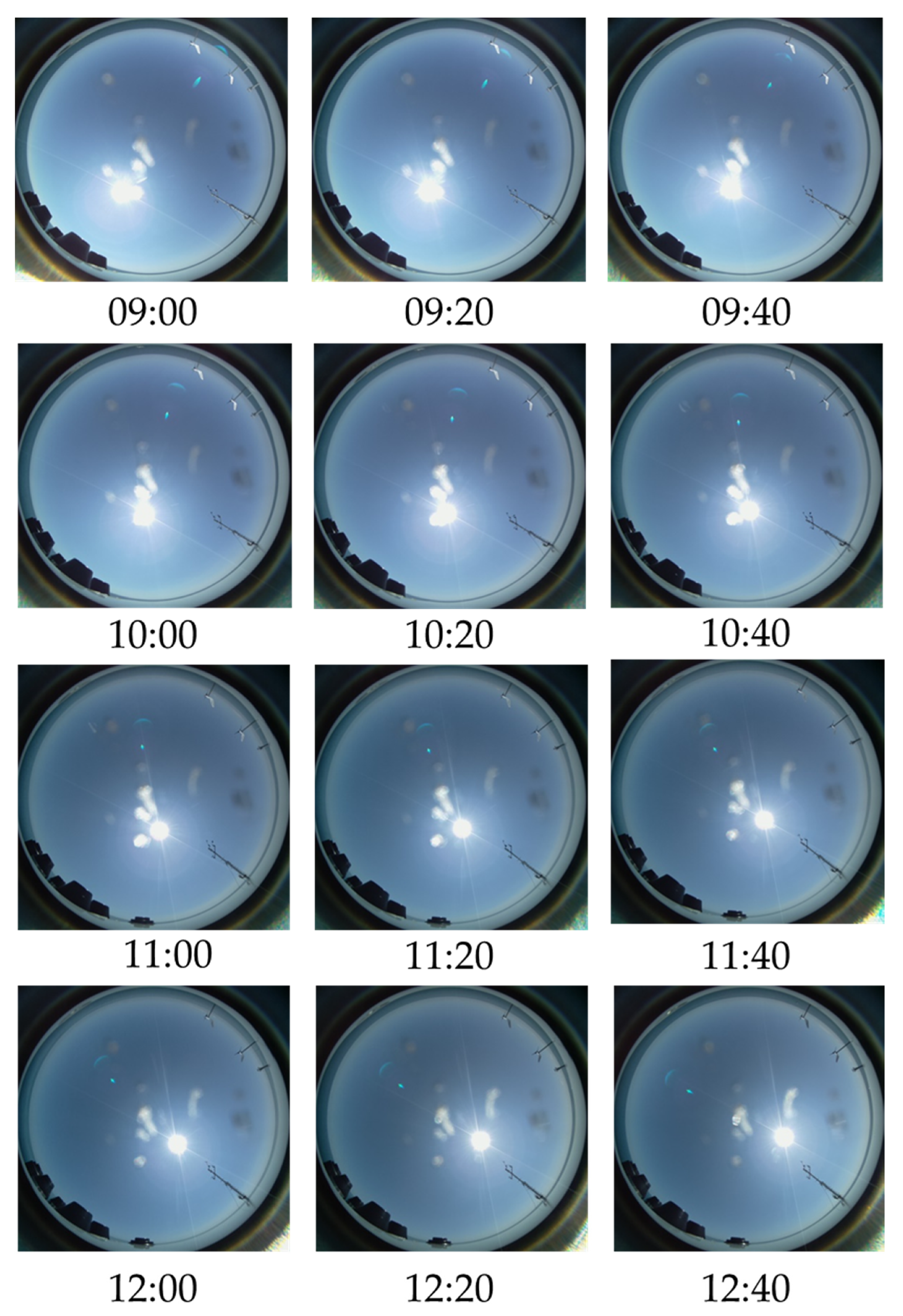
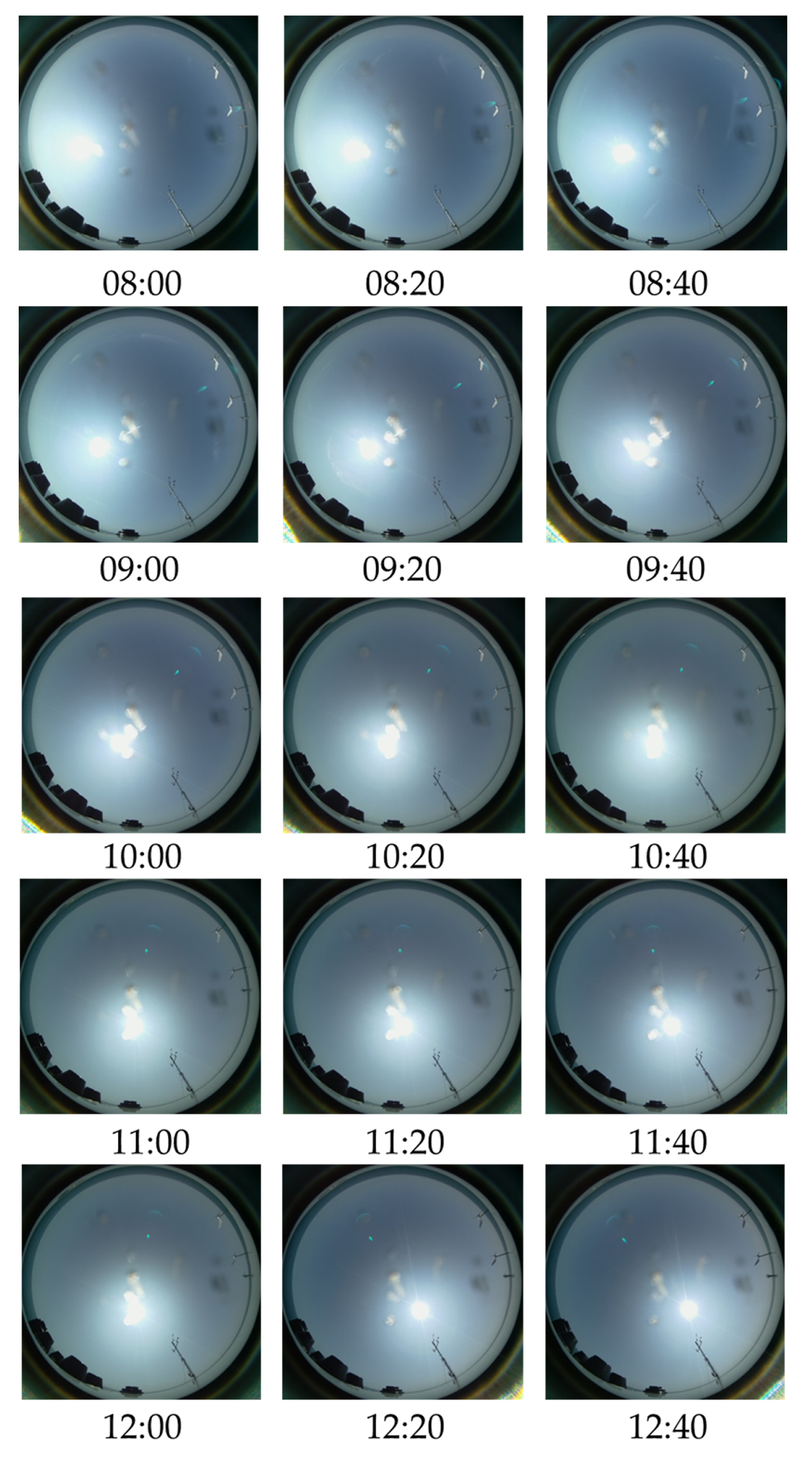
2.10. Environmental Conditions and Selection of Casts

Wind speed data was measured as part of the meteorological platform on the AAOT. Only casts with wind speeds <5 m s⁻¹ and with clear skies and no clouds, characterised from the standard deviation in $E_d$ within which there is a flat signal (Figure 4A–I), were considered in the intercomparison. Using these criteria, 13 casts were valid from 13 July, 15 casts from 14 July and 7 casts on 17 July (Figure 4).

2.11. Inherent Optical Properties and Biogeochemical Concentrations

An AC-9 absorption meter (Wetlabs, USA) with a 25 cm pathlength was used to measure particulate ($a_P$) and coloured dissolved organic material ($a_{CDOM}$) absorption coefficients as well as particulate attenuation ($c_P$) and scattering ($b_P$) coefficients every hr. Waters samples were collected from the base of the tower using a stainless steel bucket which was deployed to ~2–3 m depth and then raised by hand to the surface. One litre of the water was filtered through 0.2 µm nucleopore filters using an all-glass Sartorius filtration system. Discrete seawater samples of both filtered and unfiltered seawater were then used to measure $a_{CDOM}$ and $a_P$, respectively. The absorption of purified water (milliQ) was measured after every 10 measurements and used as a blank to correct for the absorption of water ($a_w$).

Pigment composition was analysed on triplicate samples by HPLC following the method of [64] and adjusted following [49]. In brief, samples were measured using a Waters 600 controller (Waters GmbH, Eschborn, Germany) combined with a Waters 2998 photodiode array detector and a Waters 717plus auto sampler. Details of the solvent and solvent gradient used are given in Table 1 in [49]. As an internal standard, 100 μL canthaxanthin (Roth) was added to each sample. Identification and quantification of the different pigments were carried out using the program EMPOWER by Waters. The pigment data were quality controlled according to [65]. The total chlorophyll a concentration (TChl a) was derived from the sum of monovinyl-chlorophyll a, chlorophyllide a and divinyl-chlorophyll a concentrations, although the latter two pigments were not present in these samples.

2.12. Statistical Analyses

For all above-water systems $E_d$, $L_t,$ $L_{sky}$ and $R_{rs}$ were acquired over a 5 min period for each cast. After each institute’s quality control procedure was applied (Table 2), mean, median and standard deviation values were then submitted. These were compared to the weighted mean of above-water systems that were submitted by the ‘blind’ submission date, and subsequently used as a reference. The mean of 3 × TriOS-RAMSES (RAMSES-A, -B and -C) systems was calculated, then the mean of two Seabird-HyperSAS systems (HyperSAS-A, HyperSAS-B) was calculated and from these, the weighted mean was calculated. Since HyperSAS-B were not available for all casts 1, 2, 3, 4, 5, 6, 12, 14 and 20, only HyperSAS-A data for these casts were used. In-water systems were excluded from the computation of reference values to allow a direct comparison with above-water systems and because of the lower number of comparable radiometric products.

The following statistical metrics were then computed against the reference data:

$$\mathrm{RPD}=100\frac{1}{N}{\displaystyle \sum }_{n=1}^N\frac{Rc\left(n\right)-Rr\left(n\right)}{Rr\left(n\right)}.$$

(15)

RPD is the relative percentage difference, where N is the number of measurements, Rc(n) is the institute measurement or method and Rr(n) is the reference measurement.

$$\mathrm{RMS}=\sqrt{\frac{1}{N}{\displaystyle \sum }_{n=1}^N{\left[Rc\left(n\right)-Rr\left(n\right)\right]}^2}.$$

(16)

RMS is the root mean square difference.

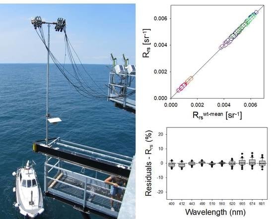
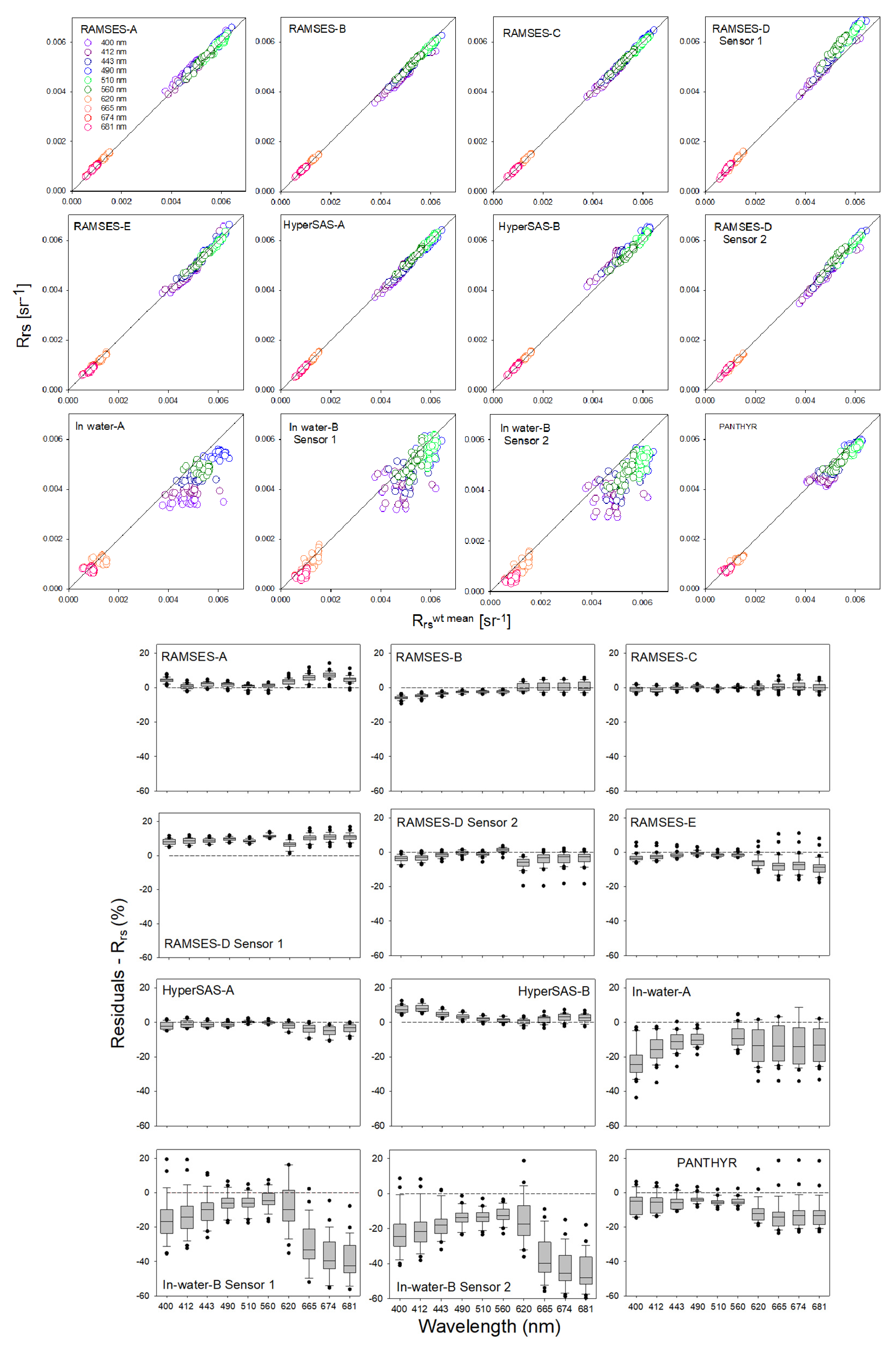
2.13. Sources of Variability in $R_{rs}$

Finally, we investigated which of the input terms in Equation (3) (i.e., $L_t, L_{sky}, E_d, {\rho }^{\prime }$) contributed most of the inter-group variability of $R_{rs}$. To this aim, we first removed the variability in $R_{rs}$ that was due to variations in environmental conditions by calculating anomalies (with respect to the median value of all measurements) of $R_{rs}$ and of $L_t, L_{sky}, E_d \mathrm{and} {\rho }^{\prime }$. We then used the standard law of propagation [2] to compute the combined variance in the anomaly of $R_{rs}$ as follows:

$$u_{R_{rs}}^2={{\displaystyle \sum }}_i{\left(\frac{\partial R_{rs}}{\partial x_i}{u}_{x_i}\right)}^2+2{{\displaystyle \sum }}_i{{\displaystyle \sum }}_j\frac{\partial R_{rs}}{\partial x_i}\frac{\partial R_{rs}}{\partial x_i}{u}_{x_i}{u}_{x_j}r\left(x_i,x_j\right),$$

(17)

where $u_{R_{rs}}^2$ is the variance in the anomaly of $R_{rs}$; $x_i$ is the anomaly of the i-th input term of (Equation (3)); $u_{x_i}$ is the robust standard deviation in the anomaly of the i-th input term; and $r\left(x_i,x_j\right)$ is the correlation coefficient between the anomalies of input terms $x_i$ and $x_j$. The term ${\left(\frac{\partial R_{rs}}{\partial x_i}{u}_{x_i}\right)}^2$ is the variance in the anomaly of $R_{rs}$ due to the variance in the anomaly of the i-th input term. The term $2{{\displaystyle \sum }}_i{{\displaystyle \sum }}_j\frac{\partial R_{rs}}{\partial x_i}\frac{\partial R_{rs}}{\partial x_i}{u}_{x_i}{u}_{x_j}r\left(x_i,x_j\right)$ are adjustments for the correlations among the input terms. We then computed the fractional contribution from the variance of each input term (as well as from the adjustment for the correlations) to the variance in the anomaly in $R_{rs}$ by calculating the ratios of each ${\left(\frac{\partial R_{rs}}{\partial x_i}{u}_{x_i}\right)}^2$ term and of the adjustment for the correlations to $u_{R_{rs}}^2$.

3. Results

3.1. Data Submission

SeaPRISM is a permanent fixture at the AAOT. Of the other nine institutes that participated in the field intercomparison, eight submitted data ‘blind’ by the submission deadline of 15 August 2018. One institute submitted their final data sets (PANTHYR and RAMSES-E) after the first results had been circulated. Of the original eight, two institutes re-processed their data. For RAMSES-D and in-water B, the irradiance Sensor 1 was found to have an angular response significantly deviating from cosine [1,4]. Data for RAMSES-D and in-water B were, therefore, re-processed using irradiance Sensor 2. The in-water B radiance sensor 2 still exhibited large deviations from the reference measurements, which was due to errors in the data processing. The final corrected in-water B data set was submitted on 3 January 2020. For HyperSAS-A the original data were submitted using a ‘Case 1 water-type’ processor which were later re-processed using a ‘case 2 type’ processor. RAMSES-B, RAMSES-C, RAMSES-D and HyperSAS-A submitted N = 35 casts. Due to problems with sensor logging at the beginning of the campaign, RAMSES-A submitted N = 34 and HyperSAS-B submitted N = 27 casts. In-water-B submitted N = 28 casts due to power outage on 13 July and on 14 July the cable for the upwelling radiance sensor broke, which led to omission of 5 casts. Due to time constraints on deployment and retrieval of the in-water-A, this institute submitted N = 28 casts.

3.2. Inherent Optical Properties (IOPs) and Biogeochemical Concentrations

Median (±median absolute deviation) and range of IOPs and HPLC TChl a during the campaign are given in

Table 3. Median and median absolute deviation of IOPs (absorption coefficients of particulate material ($a_P$), coloured dissolved organic material ($a_{CDOM}$) and water ($a_w$); scattering coefficient of water ($b_w$); attenuation coefficient of particulate material ($C_P$)) and HPLC TChl a during the AAOT intercomparison.

Quantity [Units]	Median ± abs Dev	Min–Max Range
$a_P$(440) [m−1]	0.079 ± 0.014	0.063–0.092
$a_{CDOM}$(412) [m−1]	0.112 ± 0.010	0.107–0.131
$a_{CDOM}$(440) [m−1]	0.080 ± 0.009	0.070–0.091
$c_P$(440) [m−1]	0.929 ± 0.166	0.856–1.229
$a_w\left(440\right)$ [m−1]	0.0063 ± 0.001	N/A
$b_w$(440) [m−1]	0.004 ± 0.001	N/A
TChl a [mg m−3]	0.77 ± 0.12	0.61–0.94

. $a_P$(440), c_p(440), $a_{CDOM}$(412), TChl a were slightly lower than values reported during the ARC MERIS intercomparison during July 2010 at the AAOT [17]. Notably $a_P$(440) and $a_{CDOM}$(440) were similar indicating riverine influence from neighbouring Northern Adriatic Rivers. The TChl a concentrations were typical for this site and time of year (Table 3). The standard deviation for the HPLC TChl a triplicates ranged from 1% to 9% (median and mean 5%, stdev <3%). Diel variability in TChl a was evident on 13 July and on 14 July (Figure 4M–O) and varied by 23% and 9%, respectively.

3.3. Intercomparison of $E_d\left(\lambda \right)$, $L_{sky}\left(\lambda \right)$, $L_t\left(\lambda \right)$, $R_{rs}\left(\lambda \right) and L_{wn}\left(\lambda \right)$

The variability in $E_d\left(443\right)$, $L_{sky}\left(443\right)$ and $L_t\left(443\right)$ for the days and casts used in the intercomparison are shown in Figure 4. The criteria for selection of data used in the intercomparison was a smooth $E_d\left(443\right)$ signal, indicating the absence of clouds (see also Appendix A1 for variability of these parameters on cloudy days and Figure A2 and Figure A3 for fish eye images on 13 and 14 July to show the cloud-free sky conditions). Although the conditions were clear, there were some fairly large variations in $L_{sky}\left(443\right)$. On 13 July the variation in $L_{sky}\left(443\right)$ was 40% and on 14 July it was 57%, with the largest changes at 09:20 and 10:40, respectively (Figure 4D–F). The variations in $L_{sky}\left(443\right)$ were partly due to temporal changes in sky conditions and partly due to using either 90° or 135° viewing angles (shaded areas in Figure 4D–J indicate 135° viewing angles). $L_{sky}\left(443\right)$ was always higher for both RAMSES and HyperSAS sensors (see Figure A4) with viewing angles of 90°. For example, on 14 July the viewing angle at 10:20 was 135° and was changed to 90° at 10:40. Changes in $L_t\left(443\right)$ were more uniform, indicating lower variability of in-water conditions except at 10:20 on 13 July and 10:40 on 14 July, when the changes were 20% and 35% of early morning values, respectively. Again $L_t\left(443\right)$ were consistently higher using viewing angles of 90° compared to 135° (Figure A4). The variation in $L_t\left(443\right)$ at 10:40 on 14 July co-varied with $L_{sky}\left(443\right)$, but at 10:20 on 13 July $L_t\left(443\right)$ and $L_{sky}\left(443\right)$ diverged even though the sky conditions were similar (Figure A2), possibly due to a sea surface microlayer slick. On 13 July from 12:20 to 12:40 there was a decrease in $L_t\left(443\right)$, due to a change in the viewing angle from 90° to the right to 90° to the left. Prior to 17 July there was a storm and rain on 15 and 16 July, which may change the atmospheric aerosol type and in-water conditions on 17 July, compared to those on 13 and 14 July. To further assess whether the variation in $L_{sky}\left(443\right)$ on 13 and 14 July reduced the quality of the radiometric data used in the intercomparison, across-group coefficient of variation in $R_{rs}\left(443\right)$ from the above-water systems on 13, 14 and 17 July are also presented in Figure 4J–L. The change in viewing angle from 90° to 135° and co-varying temporal changes in $E_d$, $L_t$ and $L_{sky}$ cancel out when computing $R_{rs}$ (e.g., Figure A5 and Figure A6). The $R_{rs}\left(443\right)$ coefficient of variation, therefore, represents temporal changes in both in-water constituents and the bi-directionality of the light field. This varied from 0.029 to 0.055, with the highest value recorded on 13 July at 10:40 when there was a decrease in $L_{sky}$ and increase in $L_t$. Despite the relatively large variations in $L_{sky}\left(443\right)$, the coefficient of variation in $R_{rs}\left(443\right)$ was <5.5% across above-water systems, indicating that the observed variability in $L_{sky}\left(443\right)$ was not introducing large variations in $R_{rs}$. Comparison of variations in $E_d\left(443\right)$, $L_t\left(443\right)$ and $L_{sky}\left(443\right)$ during cloudy conditions on 15 and 16 July 2018 are given in Figure A1. These data were not used for the intercomparison, but illustrate that under non-ideal conditions there are larger variations in both $E_d\left(443\right)$, $L_t\left(443\right)$ and $L_{sky}\left(443\right)$.

The intercomparison results of $E_d$ and the corresponding residuals are shown in Figure 5 and the statistics are given in

Table 4. Relative percentage difference (RPD) and root mean square (RMS) in mWm⁻²nm⁻¹ for spectral values of $E_d$ at OLCI bands 443, 560 and 665 nm. N is the number of measurements. For RAMSES-D and in-water B, S1 is Sensor 1 and S2 is Sensor 2.

Sensor Type	N	RMS 443	RPD 443	RMS 560	RPD 560	RMS 665	RPD 665
RAMSES-A	34	0.007	−1.55	0.023	−4.88	0.027	−5.74
RAMSES-B	35	0.029	6.64	0.014	3.01	0.017	3.76
RAMSES-C	35	0.006	1.13	0.005	−0.92	0.004	−0.28
RAMSES-D S1	35	0.034	−7.92	0.046	−9.66	0.048	−10.58
RAMSES-D S2	35	0.004	0.35	0.009	−1.64	0.007	−1.03
RAMSES-E	35	0.004	0.73	0.005	−1.03	0.003	−0.24
PANTHYR	30	0.007	0.85	0.011	2.18	0.018	4.07
HyperSAS-A	35	0.011	−2.30	0.008	1.61	0.004	0.78
HyperSAS-B	27	0.009	−1.79	0.005	−0.19	0.006	0.65
In-water A	28	0.005	0.03	0.014	−2.90	0.005	0.03
In-water B S1	28	0.032	−6.64	0.044	−9.04	0.046	−9.55
In-water B S2	28	0.010	1.21	0.011	−0.82	0.010	−0.22

. There was good agreement between the TriOS-RAMSES above-water systems, with an RMS <0.03 mWm⁻²nm⁻¹ across the visible spectrum and with most sensors having an RPD <5% (with some exceptions; e.g., RAMSES-A >5% at 665 nm; RAMSES-B > 6.5% at 443 nm; Table 4). There was a tendency for RAMSES irradiance sensors to over-estimate at 400 nm relative to the weighted mean, which was highest for RAMSES-B (Figure 5). RAMSES-A tended to under-estimate in red and green channels. There was a systematic bias in the RAMSES-D and in-water-B Sensor 1 $E_d$ data, compared to the weighted mean, whereby all channels were underestimated by >5% varying from ±7.9% at 443 nm to ±10.6% at 665 nm. This bias was due to poor cosine response of the sensor. To correct for this, $E_d$ from the RAMSES-D sensor 2 were processed for both RAMSES-D and in-water B data, which significantly reduced the differences against the weighted mean (Figure 6, Table 4). Due to the problems discovered with RAMSES-D and in-water B Sensor 1 data, only the corrected data using Sensor 2 are therefore plotted in Figure 5. The two Seabird-HyperSAS irradiance sensors exhibited an RMS of <0.01 mWm⁻²nm⁻¹ across the visible spectrum which was higher in the blue. Both in-water systems measured $E_d$ above-water, but tended to underestimate $E_d$. The in-water A system was within <3% at 443, 560 and 665 nm (Table 4), although it exhibited high scatter at 400 nm (Figure 5).

There was also a temporal difference between casts for the above- and in-water systems. Some outliers are observed for the PANTHYR system in Figure 5, with respect to other systems. This is thought to be due to variation of sky conditions, including sun zenith angle, between the time of the automated PANTHYR measurements and the other measurements, which were synchronized at a different time. It could also be due to the PANTHYR irradiance sensor being located on the railings rather than the mast so it may be affected by the surrounding AAOT infrastructure. The outliers in the box plots are from the first measurement taken on 14 July (Cast 14), when $E_d\left(443\right)$ was varying most quickly in time (Figure 4A).

The comparison between $L_{sky}$ measurements from the above-water systems (except PANTHYR which was viewing at different azimuth) and the corresponding residuals are presented in Figure 7 and the statistics relative to the weighted mean of the above-water systems in

Table 5. RPD and RMS in mWm⁻²nm⁻¹sr⁻¹ for spectral values of $L_{sky}$ at OLCI bands 443, 560 and 665 nm, used to quantify differences between systems and methods. N is the number of measurements.

Sensor Type	N	RMS 443	RPD 443	RMS 560	RPD 560	RMS 665	RPD 665
RAMSES-A	34	0.011	2.42	0.003	0.19	0.003	0.38
RAMSES-B	35	0.003	0.65	0.003	−0.26	0.004	−0.38
RAMSES-C	35	0.011	2.37	0.004	0.41	0.005	0.93
RAMSES-D	35	0.004	0.46	0.004	−0.49	0.005	−0.41
RAMSES-E	35	0.008	1.78	0.007	1.23	0.008	1.27
HyperSAS-A	35	0.011	−2.47	0.007	1.43	0.0041	−1.31
HyperSAS-B	27	0.005	−0.82	0.012	−2.49	0.010	−1.88

. There was very good agreement between the TriOS-RAMSES with an RMS <0.011 mWm⁻²nm⁻¹sr⁻¹ and RPD <2.5% across all channels. The Seabird-HyperSAS sensors exhibited similar results with <2.5% difference at 443, 560 and 665 nm, though HyperSAS-A at 400 nm was −5.3%. For HyperSAS-B, there was an underestimate in the green and red channels of −2.5 and −1.9%, respectively, and a slight overestimate in the 400 nm channel.

$L_t$ measurements and the corresponding residuals are shown in Figure 8, and the statistics relative to the weighted mean of the above-water systems are given in

Table 6. RPD and RMS in mWm⁻²nm⁻¹sr⁻¹ for spectral values of $L_t$ at OLCI bands 443, 560 and 665 nm, used to quantify differences between systems and methods. N is the number of measurements.

Sensor Type	N	RMS 443	RPD 443	RMS 560	RPD 560	RMS 665	RPD 665
RAMSES-A	34	0.007	1.57	0.004	−0.83	0.003	0.31
RAMSES-B	35	0.009	3.00	0.002	0.97	0.008	2.97
RAMSES-C	35	0.005	0.86	0.006	−1.21	0.003	−0.12
RAMSES-D	35	0.006	−0.57	0.005	−0.33	0.015	−2.66
RAMSES-E	35	0.005	0.39	0.007	−0.56	0.006	−0.37
HyperSAS-A	35	0.015	−2.35	0.006	1.23	0.005	−0.8
HyperSAS-B	27	0.006	1.26	0.003	−0.24	0.004	0.06

.

Again, there was good agreement between TriOS-RAMSES and Seabird-HyperSAS sensors, with RMS values generally <0.015 mWm⁻²nm⁻¹sr⁻¹ and RPD values were <3.0% at 443, 560 and 665 nm.

Similar to $L_{sky}$, at 400 nm, HyperSAS-A $L_t$ exhibited a consistent underestimate and RAMSES-A, -B, -C and –E overestimated at 400 nm (Figure 8). RAMSES-D had a low but consistent off-set from the weighted mean. For $L_{sky}$ and $L_t$ the pattern between TriOS-RAMSES and Seabird-HyperSAS was similar, but reduced compared to $E_d$, with a slight over-estimate in blue channels for RAMSES and under-estimate for HyperSAS. RAMSES-E showed a higher variability in $L_t$ compared to the other RAMSES systems, which was due to outliers on the first measurement of July 13 (Cast 1) and second measurement of July 14 (Cast 15), which correspond to low values $L_{sky}\left(443\right)$ and $L_t\left(443\right)$ or large variations in $L_{sky}$(443) (Figure 3D–H).

Scatter plots for $R_{rs}$ and the accompanying residuals relative to the weighted mean are given in Figure 9 and the accompanying statistics are given in

Table 7. RPD and RMS in sr⁻¹ for spectral values of $R_{rs}$ at OLCI bands 443, 560 and 665 nm to quantify differences in $R_{rs}$ between systems and methods. Data sets are compared against the weighted mean $R_{rs}$ from above-water systems (RAMSES-A, -B, -C, HyperSAS-A, -B). N is the number of measurements. For RAMSES-D and in-water B, S1 is $E_d$ Sensor 1 and S2 is $E_d$ Sensor 2.

Sensor Type	N	RMS 443	RPD 443	RMS 560	RPD 560	RMS 665	RPD 665
RAMSES-A	34	0.010	1.89	0.008	0.98	0.026	5.55
RAMSES-B	35	0.016	−3.39	0.011	−2.23	0.011	0.39
RAMSES-C	35	0.006	0.01	0.005	0.19	0.004	0.75
RAMSES-D S1	35	0.038	8.79	0.049	11.61	0.045	10.30
RAMSES-D S2	35	0.010	−1.63	0.008	1.34	0.027	−4.01
RAMSES-E	35	0.010	−1.46	0.004	−1.42	0.023	−7.42
HyperSAS-A	35	0.032	−1.15	0.008	−0.01	0.042	−4.02
HyperSAS-B	27	0.023	5.04	0.009	1.49	0.015	2.14
PANTHYR	29	0.032	−5.58	0.026	−5.00	0.077	−13.22
In-water A	27	0.065	−12.07	0.051	−8.20	0.097	−8.85
In-water B S1	28	0.066	−10.09	0.034	−4.39	0.19	−29.98
In-water B S2	28	0.096	−17.05	0.065	−12.30	0.229	−36.59

. Spectral comparison of $R_{rs}$ at OLCI bands for selected Casts on 13, 14 and 17 July are also given in Figure A5, Figure A6 and Figure A7. The TriOS-RAMSES and one Seabird-HyperSAS system tended to slightly overestimate $R_{rs}$ by <5% in the blue, <3% in the green, but >5% in the red (Figure 9). TriOS-RAMSES systems generally had a similar RMS in blue, green and red bands (<0.02 sr⁻¹, <0.01 sr⁻¹, <0.027 sr⁻¹, respectively) to Seabird-HyperSAS systems (<0.04 sr⁻¹, <0.01 sr⁻¹, <0.042 sr⁻¹, respectively; Table 7). For RAMSES-D, the underestimate in $E_d$ using Sensor 1 caused an overestimate in $R_{rs}$ of between 9% in the blue to 10% in the red. This was reduced to 2% and 4% respectively when Sensor 2 was used to compute $R_{rs}$. HyperSAS-A tended to underestimate $R_{rs}$, where the RPD at 443 nm was −1.5% and at 665 nm was −4%. The PANTHYR system showed consistent precision with an RMS <0.032 sr⁻¹ at the blue and <0.026 sr⁻¹ at green bands, with differences from the weighted mean of $R_{rs}$ of <5.6% at 443 nm, <5% at 560 nm, and 13% at 665 nm (Table 7). The in-water systems underestimated $R_{rs}$, and they exhibited a high scatter and bias compared to the weighted mean of the five above-water systems (see also magnitude and shape of In-water spectra in Figure A5, Figure A6 and Figure A7). For in-water A, the difference was <10% across visible bands. For in-water B Sensor 2, the RPD and RMS were −17% and 0.1 sr⁻¹ at 443 nm and 12.3% and 0.065 sr⁻¹ at 560 nm, respectively. These differences may in part be due to comparisons against a weighted mean from some of the above-water systems. For in-water B, the effect of using an $E_d$ sensor with poor cosine response on $R_{rs}$ (Sensor 1), gave higher values which fortuitously agreed better with the weighted mean of the above-water systems in blue and green bands (RPD of 10% at 443 nm and 4% at 560 nm). For $R_{rs}$ red bands, both in-water B Sensor 1 and 2 the difference was much higher (~30%).

For $L_{wn}$, SeaPRiSM was used as an independent reference for both above-water and in-water systems rather than the weighted mean from three of the TriOS-RAMSES and two of the Seabird HyperSAS systems. There were, however, only nine near-coincident casts with SeaPRiSM during 13, 14 and 17 July 2018 and this was reduced to six casts for HyperSAS-B and in water-B. PANTHYR was not compared with SeaPRiSM, due to the differences in relative azimuth angles and the BRDF correction used for RAMSES and HyperSAS systems. TriOS-RAMSES systems tended to underestimate $L_{wn}$, which was generally <8.0% at 441 nm with an RMS <0.052 mWm⁻²nm⁻¹sr⁻¹, <6.0% at 551 nm and an RMS <0.031 mWm⁻²nm⁻¹sr⁻¹ and <9.5% at 667 nm and RMS <0.057 mWm⁻²nm⁻¹sr⁻¹ (Figure 10,

Table 8. RPD and RMS for spectral values of $L_{wn}$(λ) at SeaPRiSM bands 441, 551 and 667 nm, used to quantify differences between systems and methods compared to AERONET-OC $L_{wn}$(λ). For RAMSES-D and in-water B, S1 is Sensor 1, S2 is Sensor 2.

Sensor Type	N	RMS 441	RPD 441	RMS 551	RPD 551	RMS 667	RPD 667
RAMSES-A	9	0.046	−6.32	0.009	−0.83	0.057	9.45
RAMSES-B	9	0.051	−7.89	0.031	−5.82	0.046	2.55
RAMSES-C	9	0.011	−3.49	0.004	−3.69	0.005	4.73
RAMSES-D S1	9	0.037	1.22	0.027	5.10	0.064	9.00
RAMSES-D S2	9	0.048	−6.00	0.020	−2.59	0.052	−0.10
RAMSES-E	9	0.052	−5.65	0.030	−5.62	0.055	−5.90
HyperSAS-A	9	0.048	−5.52	0.021	−3.94	0.064	−4.81
HyperSAS-B	6	0.025	−1.39	0.041	−7.37	0.058	3.99
In-water A	8	0.063	−11.51	0.051	−10.25	0.071	−9.06
In-water B S1	6	0.039	−3.38	0.036	−3.18	0.164	−17.44
In-water B S2	6	0.069	−10.49	0.043	−4.71	0.200	−24.67

). The HyperSAS systems also underestimated $L_{wn}$ compared to SeaPRISM which were between −1.4% and −5.5% at 441 nm, −4.0% and −7.5% at 551 nm and <5.0% at 667 nm.

In-water A exhibited a −10.2% difference across 441, 555 and 667 nm bands. In-water B Sensor 2 exhibited smaller differences at blue and green bands with an RMS 0.11 to 0.23 mWm⁻²nm⁻¹sr⁻¹ and RPD of −10% and −5% at 441 nm, respectively. At 667 nm, the RPD for in-water B was more than double that of in-water A (Table 8). For in-water B using $E_d$ Sensor 1, $L_{wn}$ was higher and more accurate than Sensor 2. This was probably caused by the extrapolation of $L_u$ from in-water profiles to above surface which compensated the error in $E_d$ due to non-normal cosine response for Sensor 1.

4. Discussion

Using a stable measurement platform, under near-ideal illumination and environmental conditions to compare a range of above-water optical measurement systems, there was generally <6% difference in $E_d$ among sensors with an RMS <0.03 mW m⁻² nm⁻¹. This was also the case for the sole instrument deployed on a ship (in-water A), for which the unavoidable tilt can introduce additional uncertainty. In a previous intercomparison at the AAOT, [17] reported similar differences between two TriOS-RAMSES sensors and the WiSPER system, which were <5.5% at blue, green and red wavebands. In this study, compared to the weighted mean, TriOS-RAMSES tended to slightly overestimate, and Seabird-HyperSAS slightly underestimated $E_d$ (Table 4), also reported by [4]. These differences were always greater at 400 nm for both types of $E_d$ sensors (Figure 5). The weighted mean does not represent the true value of $E_d$, so we can only conclude that the RAMSES and HyperSAS sensor types are different, particularly at 400 nm. This wavelength is also where the highest uncertainty is expected for calibration coefficients, since at 400 nm the calibration lamp signal is at its lowest. The greatest difference was for RAMSES-D, in which Sensor 1 exhibited a systematic bias (Figure 6), due to a poor cosine response of the $E_d$ sensor (see also sensor 81EA data in Figures 13 and 15 of [4]). By contrast, RAMSES-D Sensor 2 had an appropriate cosine response (sensor 81E7 in [4]), and performed similarly to the other $E_d$ sensors. In the absence of this field inter-comparison the poor cosine response may have been used unchecked for satellite validation. The <6% difference observed for the other sensors may arise from smaller differences in cosine response among or between sensor types [4], as well as from the temperature effects of individual and specific sensors. Even within a single sensor type, cosine response may be quite different from unit to unit, as shown by [66]. For the in-water systems, the differences were also low and generally <2.5%. Similar to the study of [17], the sensors were pre-calibrated at the same laboratory [1] and potential biases due to differences in the calibration coefficients from different sources were, therefore, removed. This contributed to the small differences in $E_d$ between sensor types and methods, both above- and in-water.

For radiance measurements, the differences in above-water $L_{sky}$ over visible bands compared to the weighted mean, except at 400 nm, were <2.5% with an RMS <0.01 mWm⁻²nm⁻¹sr⁻¹ (Table 5). The differences between RAMSES and HyperSAS sensors were similar at blue bands and higher for HyperSAS in green and red bands. The differences within RAMSES sensors were generally small, with one group showing a slightly higher deviation. This may in part arise from the processing methods used and specifically the number of replicates processed per cast (Table 2), especially in view of the high variability in $L_{sky}$ (Figure 4). This is further discussed in Section 4.1.5. For $L_t$, the differences for both above-water sensor types were <3.5% with an RMS <0.009 mWm⁻²nm⁻¹sr⁻¹. The differences in $L_t$ in the blue and green for RAMSES and HyperSAS were similar, but were lower for HyperSAS in the red where the signal is lower (Table 6, Figure 8).

Of the radiometric quantities measured, $E_d$ showed the largest variation between sensor types and methods, and the differences in $L_{sky}$ and $L_t$ between above-water sensor types were smaller. In this study, the differences between sensors were smaller than [4] who made the measurements under heterogenous (partially cloudy) conditions. The factors below contribute to the differences found.

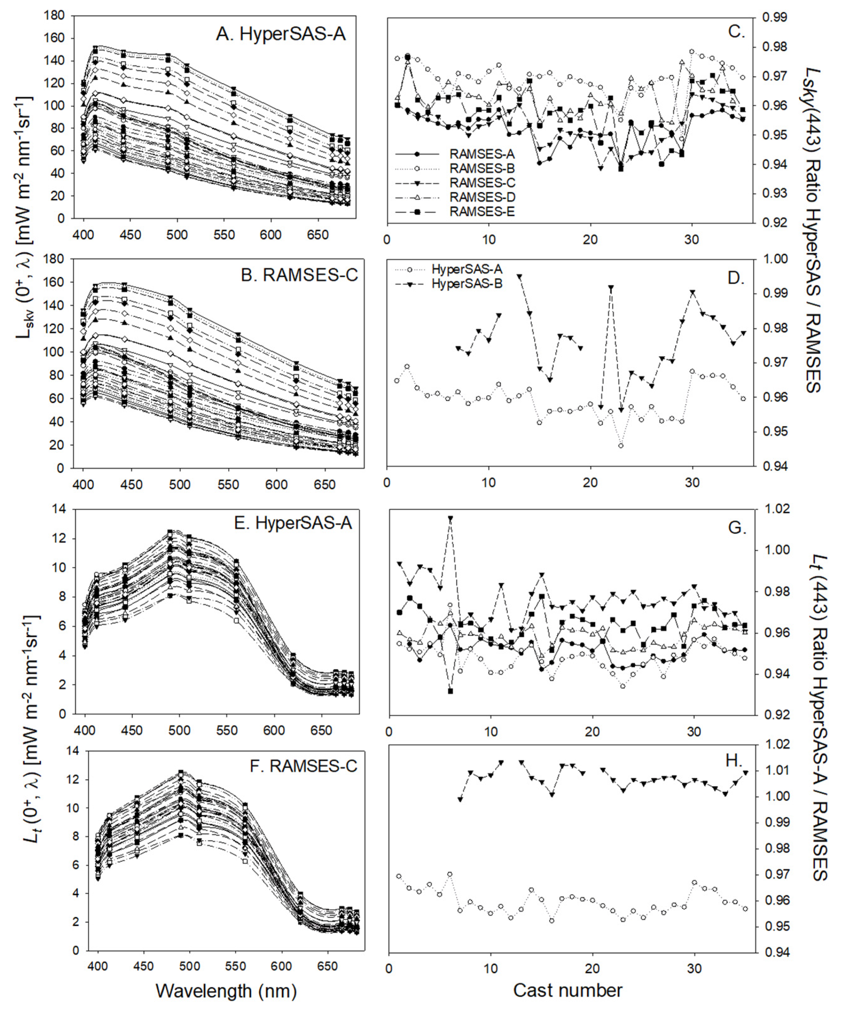
4.1. Sources of Uncertainty

4.1.1. Effects of Sensor Absolute Calibration

All sensors were calibrated at UT in June 2018 under the same laboratory conditions, using the same calibration standards and by the same operator prior to the field intercomparison. Standard uncertainty of the calibration coefficients were of the order of 1% for irradiance and radiance over the whole spectrum. Potential biases due to differences in the calibration coefficients from different sources were therefore removed. According to [1], the long term stability of the calibrations was good with 80% of the sensors experiencing a change of <1% over one year. The largest differences in $E_d$ were at 400 nm especially for two of the RAMSES sensors (RAMSES-B, RAMSES-E) and the two HyperSAS sensors. RAMSES-B and -C, HyperSAS-A and -B $E_d$ sensors were the oldest used for the intercomparison (Table 2). Both RAMSES and HyperSAS have redesigned the geometry of the sensor head over time possibly suggesting that the deviation at blue bands may in part be due to the age and geometry design of the cosine collector. These effects were not visible over one year of calibration [1]. For $L_{sky}$ and $L_t$ there was a similar trend at 400 nm, but the magnitude of the difference was much lower for both RAMSES and HyperSAS sensors. These effects need to be carefully tracked through full and regular sensor characterisation, especially for the $E_d$ sensors.

4.1.2. Differences in Cosine Response

The largest difference in measured $E_d$ was found in the RAMSES-D $E_d$ Sensor 1, in which a poor cosine response caused a high bias in the measurements. As highlighted in [4], the RAMSES-D Sensor 1 had large cosine error of 10–12% in the visible channels, which resulted a negative bias of ~12% at 400 nm and 7–10% in bands >490 nm (Figure 6). The angular dependence of responsivity of the irradiance instrument should correspond to the cosine of incidence angle, but for the RAMSES-D Sensor 1 this was not the case (see also Figures 13 and 15 in [4]). This caused the overestimate and offset in $R_{rs}$ over all spectral bands for RAMSES-D (Figure 9). In addition, [4] highlighted that the manufacturer’s specification of the Seabird-HyperSAS [67] is that the cosine RMS error is <3% at 0–60°, and within 10% at 6–85° incidence angles and that for TriOS-RAMSES [68], the accuracy is between 6–10% depending on spectral range. It is noted, however, that the manufacturer specifications are vague and laboratory measurements on individual radiometers can show quite different behaviour [66]. For the Biospherical $E_d$ sensor the cosine response was measured in February 2014 by the manufacturer and the average cosine error was <2% at 0–60° and within 9% at 60–85°. Deviations from these may be one of the main sources of error contributing to the differences in the field measurements. The cosine response is likely to be the principal cause of the differences between and among sensor types.

4.1.3. Differences in Field of View (FOV) of Radiance Sensors

For all TriOS-RAMSES radiance sensors, the manufacturers state that the FOV is 7° (Table 2). For the Seabird HyperSAS sensors used in this study, FOV is 6°. Theoretically there should be small differences due to the FOV between TriOS-RAMSES and Seabird HyperSAS-A radiance sensors. Instrument-specific differences between the sensors may however, contribute to the differences in $L_{sky}$ observed. This is illustrated in Figure 7 of [4], especially when sky conditions are heterogeneous, with partial clouds, in the viewing direction. In this study, instrument specific differences may be more difficult to distinguish, since the sky conditions were cloud-free and stable (Figure A2 and Figure A3). In addition, the above-water systems were mounted on the same frame so in theory they were viewing the same area of sky, although differences may arise from instrument-specific FOV or alignment differences of the sensors [4]. To assess the difference due to FOV, firstly $L_{sky}$ spectra for each cast from one of the TriOS-RAMSES systems (RAMSES-C; FOV 7°) are compared with those from Seabird-HyperSAS-A (FOV 6°; Figure 11).

In general, and especially for casts with $L_{sky}$(443) >100 mWm⁻²nm⁻¹sr⁻¹, Seabird-HyperSAS-A (Figure 11A) was slightly lower than RAMSES-C (Figure 11B), suggesting possible differences in FOV. To verify this trend, the ratio between $L_{sky}$(443) HyperSAS-A/$L_{sky}$(443) RAMSES for each cast is plotted for each RAMSES sensor (Figure 11C) and then for HyperSAS-A and –B against the mean of the RAMSES sensors (Figure 11D). In theory, the ratio between $L_{sky}$(443) HyperSAS-A or -B/$L_{sky}$(443) RAMSES should be close to 1, since HyperSAS have a similar FOV (6°) compared to RAMSES (7°). Compared to individual RAMSES sensors and the mean of the RAMSES sensors, HyperSAS-A and -B $L_{sky}$(443) are consistently lower. Compared to the RAMSES mean, HyperSAS-A is consistently lower than HyperSAS-B, further suggesting that the small differences in FOV between HyperSAS and RAMSES have an impact on the observed differences. The influence of the number of replicates used to compute median $L_{sky}$ values (Table 2) and the integration time used during these measurements will also contribute to these differences. In theory, this effect should also be seen in the $L_t$ radiance measurements. In Figure 11E–H the same $L_t$ data as for $L_{sky}$ are presented. The difference between HyperSAS-A and –B and RAMSES is less apparent for $L_t$ than it is for $L_{sky}$ (Figure 11A–D). The ratio between $L_t$(443) HyperSAS/$L_t$(443) mean RAMSES is clearly lower for HyperSAS-A compared to HyperSAS-B, further suggesting that differences may be due to these small variations in FOV. This is specific to the conditions during this intercomparison, under clear skies and on a stable platform. Figure 7/C23 of [4] shows variation of sky reflection for different FOV sensors. In addition, Figure 6 of [7] shows that the reflectivity of the sea surface varies strongly and non-linearly over an angular range of 23° around the 40° incidence angle, suggesting that a smaller FOV is preferable for these measurements. Under non-homogeneous sky and sea conditions and on moving vessels, the different FOV could generate greater differences in both $L_{sky}$ and $L_t$. This warrants further investigation.

4.1.4. Temperature Effects

Variations in temperature can affect the performance of the radiometer photo-diode array which can have a significant effect on the uncertainty of the instrument [69]. For TriOS-RAMSES sensors, temperature coefficients vary from −0.04 × 10⁻² °C⁻¹ at 400 nm to +0.33 × 10⁻² °C⁻¹ at 800 nm [69]. For biospherical microradiometers, typical temperature coefficients of −3.65 × 10⁻⁴ °C⁻¹ have been reported [48]. Temperature can affect the dark and light counts of an instrument, across spectral regions differently. In this intercomparison, the calibration temperature (at the University of Tartu) was 20 °C, whereas the air temperature at the AAOT from 13–17 July 2018 varied from 23 °C to 26 °C. Due to heating of the metal super-structure of the AAOT and the sensor body, the internal temperature of the photo-diode array may have been considerably higher than 26 °C. The internal temperature of HyperSAS-B was far higher (~40 °C). Vabson et al. [4] identified that differences in calibration and ambient temperature during field intercomparisons may contribute to the bias in the results. Due to the small difference between the calibration and ambient temperature at the AAOT, theoretically the bias should be smaller, however the internal temperature of each sensor type may respond differently under the same air temperature. The Seabird-HyperSAS sensors are manufactured from plastic with a black finish and have a larger volume, whereas the TriOS-RAMSES are fabricated from stainless steel with a metallic finish and have a smaller volume. The biospherical surface reference sensor is manufactured from plastic with a white painted finish. Although temperature biases should be similar to all sensors with the same internal spectrometer, the design characteristics of TriOS-RAMSES versus the Seabird-HyperSAS may alter the internal temperature of each instrument type with respect to the ambient temperature, which could result in biases between instrument types. Due to the black finish, the HyperSAS sensors used in this study may have a higher internal temperature, which may account for some of the differences seen. In addition the RAMSES power consumption is smaller compared to the HyperSAS sensors, which may contribute to varying the internal temperature of the instrument. Theoretically, the differences should increase throughout the day from the morning casts into the afternoon as the sensors heat up over the course of the day. This needs to be carefully characterized and verified in future intercomparisons.

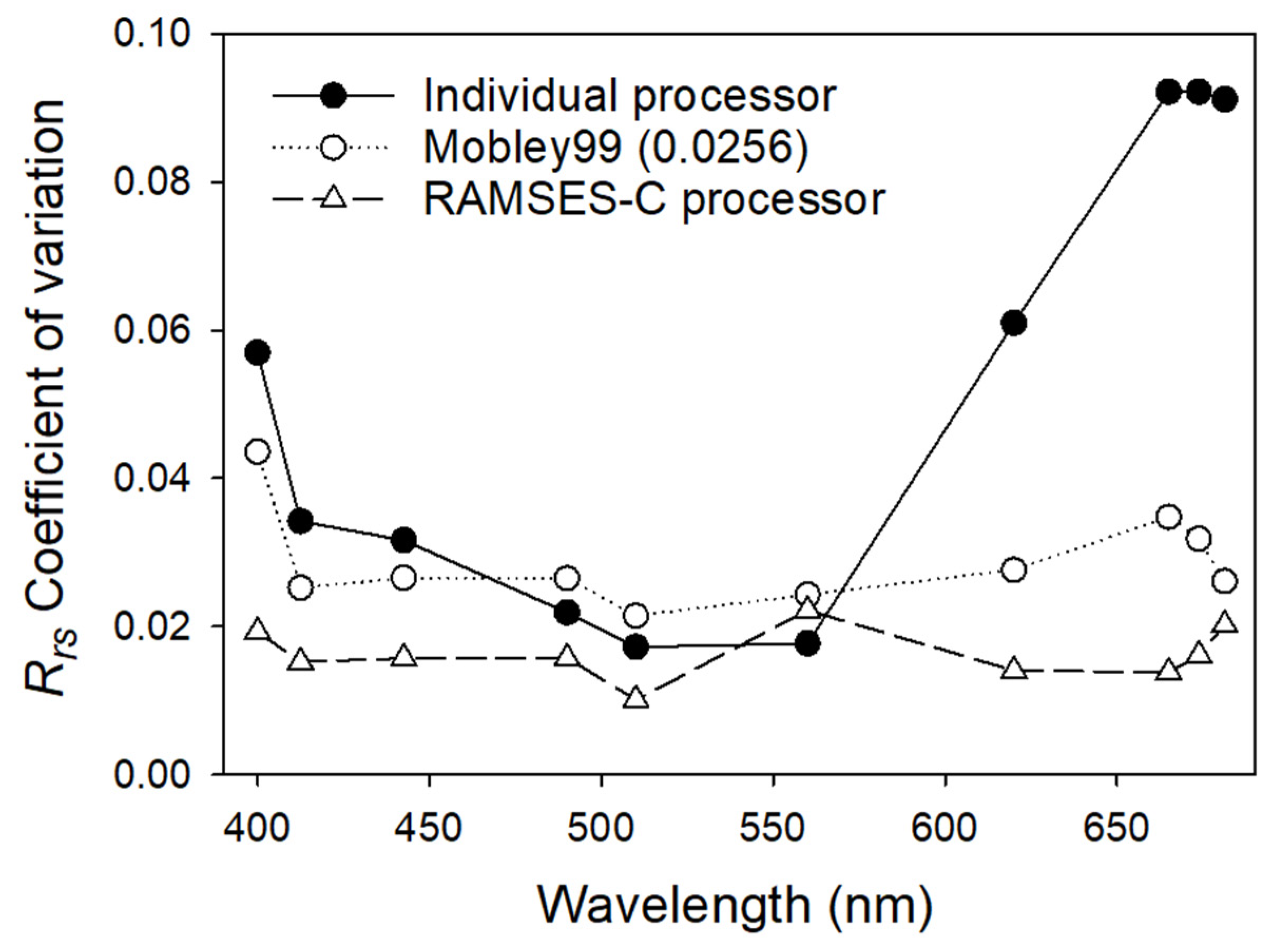
4.1.5. Differences Due to Data Processing

The differences among sensor systems may arise from the diverse methods of processing and quality control in data implemented between institutes. The procedure for data processing includes quality control of measured data, time binning, spectral interpolation and applying appropriate Fresnel reflectance factors, ${\rho }^{\prime }.$ The main differences in data processors between systems are summarised in Table 2. Of the TriOS-RAMSES processors, RAMSES-A and -B used the same number of replicates for $E_d$, $L_{sky}$ and $L_t$ and ${\rho }^{\prime }$ to process $R_{rs}$ (Table 2). RAMSES-E used a different number of replicates for $E_d,$ $L_{sky}$ and $L_t$, a different ${\rho }^{\prime }$ to process $R_{rs}$, and added NIR correction to the processing. For RAMSES-C and RAMSES-D Sensor 2 there were large differences in the number of replicate $E_d$, $L_{sky}$ and $L_t$ used, though RAMSES-D used RAMSES-C $L_{sky}$ measurements. To assess the effect of differences between processing chains, we assessed two steps in the processing for one Cast (Cast 7). Firstly, a subset of TriOS-RAMSES data (RAMSES-B, -C, -E) were run through one processing chain (that of RAMSES-C) to assess the differences in $R_{rs}$ due to processing methods (Figure 12). The differences are only significant at red bands and increase from 620 to 685 nm. Across blue to green bands, the differences are minimal. Using the individual processors, the difference over visible bands for RAMSES-B, and -E compared to RAMSES-C were 3.45%. By comparison using the RAMSES-C processor for all three datasets reduced the difference to 1.31%. For TriOS-RAMSES systems, differences in processors therefore only accounted for ~2% in the blue and green, but up to 8% in the red. Secondly, for Cast 7 we evaluated the differences in processing due to the ${\rho }^{\prime }$ value used by each institute against using a single ${\rho }^{\prime }$ factor (Figure 12). Using the same ${\rho }^{\prime }$ value, the difference was reduced to ~1% at red bands. The difference between using a single ${\rho }^{\prime }$ value was, therefore, as important as using a common processor, but the effect was only significant for red bands. Although a common processor has been advocated for use in the future, this study suggests that the use of common ${\rho }^{\prime }$ values for RAMSES systems is the important aspect for reducing differences between institutes. The use of the same ${\rho }^{\prime }$ for the in-water A system would also be beneficial in reducing differences in $R_{rs}$ of about 1.7%. Further work should focus on deriving ${\rho }^{\prime }$ values from in-water and above-water measurements.

4.1.6. Differences between Case 1 and Case 2 Water-Type Processors

NIR reflectance is expected to be close to zero in waters with low particle scattering [10]. There has been much discussion in the literature around this topic, and the assumption for Case 1 waters where particle scattering is considered low and application to Case 2 waters where it can be significant. An offset from zero in the NIR has been attributed mainly to residual surface water effects (spray, sun glint, whitecaps, and sky radiance including scattered cloud reflected on waves). Any offset observed in the NIR that is not due to particle scattering is expected to be spectrally neutral and can be compensated for by subtracting this signal from the $R_{rs}$(λ). For high particle scattering, the shape of $R_{rs}$(λ) should reflect the spectral dependence of the reciprocal of water absorption [42]. If this is not the case, high particle scattering cannot account for the NIR offset and may thus be subtracted. In Figure 13, the effect of not including and including NIR correction on HyperSAS-A data are compared for three casts (1, 4, 20). When NIR correction is included, the shape of the HyperSAS-A spectra at OLCI bands are closer to the in-water A spectra (Figure 13A–C). When the NIR correction is not implemented the shape of the HyperSAS-A spectra are closer to the mean of the RAMSES spectra (Figure 13D–F). We have to consider which of the $R_{rs}$(λ) spectral shapes are correct; the above-water or in-water? As an independent measurement, we have referenced each system to SeaPRiSM, although this is also an above-water system. Zibordi et al. [17] showed however, that SeaPRISM $L_{wn}$ are within −0.1% of in-water WiSPER measurements. Although we have no measurements from WiSPER in this study, in-water A compare well with SeaPRISM with a slight under-estimate of up to 10% at 441, 551 and 667 nm (Figure 10; Table 8). This possibly suggests that NIR correction for these waters may be necessary. The difference between applying or not the NIR correction on HyperSAS-A data compared to SeaPRiSM is given in Figure 13G,H. HyperSAS-A with NIR correction resulted in a consistent under-estimate in $L_{wn}$ over visible bands, although the scatter was small. For HyperSAS-A with no NIR correction, the data were closer to the 1:1, although the scatter increased. This suggests that no NIR correction, at least for HyperSAS-A, is recommended.

4.1.7. Other Effects

A number of other effects that may have caused significant differences between the sensors have already been considered in detail by [4]. Of these, the impact of the stray light in field measurements is expected to have the greatest effect, which was higher in the blue (<3.5%), and smaller in green and red (<1%). Data interpolation effects during processing can sometimes cause discrepancies. For example the interpolation of the radiometric measurements to OLCI bands is reported to contribute <0.5% of the variance between sensors except at 400 nm where the variance is expected to be larger. This depends however on whether the interpolation is done on the irradiance and radiance parameters that are used to compute reflectance or on the reflectance data directly. If on the latter, the error can be 5% [70]. No large difference between multi- and hyperspectral $E_d$ data were observed (Figure 4), however the uncertainty related to the band shift needs to be assessed further. Polarization, the effect of light exhibiting different properties in different directions, is considered to be smaller still (<0.25%) [4].

4.2. Differences in $R_{rs}\left(\lambda \right)$ and $L_{wn}\left(\lambda \right)$

For $R_{rs}$ the mean absolute differences among TriOS-RAMSES systems were 2.5% at 443 nm, 2.0% at 560 nm and 8% at 665 nm. In a previous study, [17] compared $R_{rs}$ from two TriOS-RAMSES sensors against a WiSPER at the AAOT in 2010 and found that the RPD was <8% at 443 nm, <4% at 555 nm and <11% at 665 nm. The WiSPER was not available to us as an independent reference. However, the above-water sensors that we deployed were located side by side on the same measurement frame with the ability to turn them away from the sun and shade, as opposed to being fixed on the railings of the AAOT in the [17] intercomparison. For Seabird-HyperSAS the differences in $R_{rs}$ were 3.1%, 0.75% and −3.1%, respectively. Only two HyperSAS systems were compared as opposed to five for TriOS-RAMSES, so the lower variability for HyperSAS is expected. The PANTHYR system showed consistent precision, with differences from the weighted mean of $R_{rs}$ of <2.5% in the blue, <3.0% in the green, and <5.5% in the red. Since the PANTHYR was pointed at a different water area than the other sensors during the intercomparison, this result is promising. The differences in $R_{rs}$ were higher between above- and in-water methods, though interpretation of this is compounded by the fact that the reference measurement was from above-water systems only. For the in-water systems the RPD were within 11% at 443 nm, 7.5% at 560 nm and up to 17% at 665 nm, respectively. A large part of the difference comes from the application of BRDF correction to account for the angular response of variation of upwelling light measured by the above-water systems. In addition, the in-water A and B casts did not match exactly with the above-water casts in either location or time, and fewer casts were made in-water.

For the comparison against SeaPRISM data, we eliminated these potential biases by performing BRDF correction to all above-water systems, to compute $L_{wn}$ (Figure 13). The SeaPRISM has a long established legacy as a FRM and for satellite validation and therefore provides high quality data to compare to each system. All above water systems showed a similar pattern with a slightly lower $L_{wn}$ in the blue and green compared to SeaPRISM. The TriOS-RAMSES systems showed a slightly lower difference in $L_{wn}$, which was generally <8%, <6% and <9.5% at 441, 551 and 667 nm, respectively. The differences were probably caused by a combination of imperfect correction of sky glint, propagation of differences in $E_d$ and radiometer calibration and characterization. For HyperSAS, the difference compared to SeaPRiSM were <6%, <8% and <5% at 441, 551 and 667 nm, respectively. For in-water A and in-water-B, there were differences of 10 and 13% respectively, compared to SeaPRiSM across the 441, 551 and 667 nm bands. Processing of the in-water data requires instrument self-shading correction [71,72]. An in-water correction for instrument self-shading of $L_u$ and shading by the deployment cage was not performed for in water-B, which is likely to account for a significant proportion of the error, especially in the red bands. In addition for in water-B, the influence of scattered light from the deployment frame, significant influence of the deployment cable on the light field, or the influence of the AAOT super-structure on the in-water light field and extrapolation of $L_u$(z, λ) to $L_{wn}$, were not accounted for. If these effects were corrected for, undoubtedly the comparison with SeaPRiSM would have improved. Moreover, the use of a Case 1 water model for deriving $L_u$ from irradiance measurements in complex waters is likely to introduce further uncertainty [60]. Further uncertainties for in-water $L_{wn}$ data may result from extrapolating the measured spectra at deeper depths to the surface in order to obtain the subsurface radiance (in-water B) or from the approximation of converting the subsurface upwelling radiance ($L_u$) to $L_{wn}$. A proportion of the difference between the above-water and in-water system and SeaPRiSM will be due to differences in the exact time of casts and interpolation over them.

No uncertainty budget was calculated for each individual sensor or system during this intercomparison. Vabson et al. [4] computed the relative uncertainty of the same above-water sensors under field conditions at an Estonian Lake. The relative uncertainty for irradiance sensors varied from 9.7% to 4.7% from blue to red bands. For $L_{sky}$ and $L_t$, the uncertainty was ~2% and 4%, respectively across visible spectral bands. This study and that of [4] are similar. Both use the same sets of radiometers, and the same procedures to calibrate them. Differences arise from the environmental conditions especially temperature and the repeatability of the measured signal. Both studies do not however, characterise stray light and non-linearity which may be different under the different environmental conditions experienced. The uncertainty budget of differences between radiometers during this study is, therefore, likely to be similar to the budget given in [4]. Zibordi et al. [17] included an uncertainty budget for each measurement system and compared relative uncertainties for each against the reference system. They found that the differences between methods and systems could be explained by the combined uncertainties determined for the systems compared [17].

4.3. Propagation of Errors in $E_d\left(\lambda \right)$, $L_{sky}\left(\lambda \right)$ and $L_t\left(\lambda \right)$ to $R_{rs}\left(\lambda \right)$

We evaluated which of the individual inputs terms in Equation (3) contributed the greatest fraction of the variance in $R_{rs}$ (Figure 14). From 400 nm to 610 nm, $E_d$ accounted for the largest fraction variance in $R_{rs}$. At 443 nm, both $E_d$ and $L_t$ accounted for a similar fraction of the variance in $R_{rs}$.

Wavelengths higher than 610 nm, the contribution of ${\rho }^{\prime }$ (given as Rho in Figure 14) became dominant. $L_{sky}$ consistently exhibited the lowest contribution to the variance in $R_{rs}$ which was <3% over the visible spectrum.

The adjustment for the correlations among the input terms also contributed a relatively large fraction of the variance in $R_{rs}$. The sign of the adjustment was negative indicating that the correlation terms decrease the variance in $R_{rs}$. Overall this analysis showed that minimizing the errors arising from the measurement of $E_d$ is the most important variable for reducing the inter-group differences in $R_{rs}$.

Recommendations: This field intercomparison illustrated that the differences in $E_d,L_{sky}\mathrm{and}{L}_t$ were low and generally less than the target 5%, although there were some anomalies above this for individual sensors and bands. The exercise was also pivotal in highlighting some errors in protocols and anomalies arising from some sensors. The difference in $E_d$ between systems was the highest, which was greater for RAMSES (<7%) compared to HyperSAS (<2.5%) irradiance sensors. For $L_{sky}$ the differences were low and similar at blue bands for RAMSES and HyperSAS but higher in green and red bands for HyperSAS. For $L_t$, differences in the blue and green for RAMSES and HyperSAS were similar, but lower for HyperSAS in the red. The differences in $E_d$ are likely due to differences in cosine response of individual sensors. Differences in $L_{sky}$ and $L_t$ are possibly due to a combination of differences in viewing geometry, angular response and temperature effects between the sensors plus processing methods used. In this study, we could not isolate all of these factors to evaluate the magnitude of their effect individually. Recommendations for future intercomparisons are as follows:

• For both above- and in-water systems, the cosine collector of the $E_d$ sensor needs to be carefully characterised to ensure the most accurate measurements are made.
• We found that above-water Fresnel reflectance factor ${\rho }^{\prime }$ caused a high variability between processing chains which was greater than other differences between processors, as demonstrated by using a single community processor. Future studies should assess further differences between above and in-water systems and the resulting ${\rho }^{\prime }$ under a range of environmental conditions and on moving vessels.
• The experimental design should be carefully considered in order to balance between representative sensor types of different above-water, in-water, and new technological systems whilst capturing a broad international range of participants that are active in satellite ocean colour validation.
• This intercomparison focused mainly on differences within and between TriOS-RAMSES systems. Differences within RAMSES systems were low. Future intercomparisons should include a wider range of sensors and systems to capture a further cross-section of the community, rather than just RAMSES systems.
• A more detailed characterisation of stray light, cosine response, linearity, temperature response and polarization sensitivity of individual instruments should be made to assess the contribution of each of these factors to the overall measurement uncertainty. Once these have been assessed, it is recommended to compute a full uncertainty budget as demonstrated in [4,17,73], to evaluate relative differences in uncertainty between instruments.
• Differences between sensors with varying FOV should be further investigated under non-homogeneous sky and sea conditions. In particular the use of a large FOV may be suboptimal when viewing the sea surface which has strong angular variability at the viewing nadir angle of 40°.
• Further intercomparisons of this nature are required from other types of platforms, such as on moving ships as in [74], and under non-ideal environmental conditions such as high sea states and partially cloudy skies when the errors between sensors are expected to increase.

5. Conclusions

A field intercomparison was conducted at the Acqua Alta Oceanographic Tower (AAOT) in the northern Adriatic Sea, from 9 to 19 July 2018, to assess combined differences in the accuracy of measurements collected using a range of in- and above-water optical systems. Prior to the intercomparison, the absolute radiometric calibration of all sensors was carried out using the same standards and methods at the same reference laboratory (University of Tartu) and the same operator. Measurements were performed at the AAOT under near-ideal conditions, on the same deployment platform and frame, under clear sky conditions, relatively low sun zenith angles and moderately low sea state (<5 m s⁻¹). For $E_d$, there was generally good agreement with differences of <7% between institutes with an RMS of <0.03 mWm⁻²nm⁻¹, except for one $E_d$ sensor which exhibited a systematic bias in the data due to poor cosine response. The difference in $E_d$ was greater for RAMSES than for HyperSAS sensors. For $L_{sky}$ and $L_t$ the differences between systems and institutes were consistently lower. For $L_{sky}$, the differences were <2.5% with an RMS <0.01 mWm⁻² nm⁻¹sr⁻¹, and RAMSES and HyperSAS sensors were similar at blue bands, but HyperSAS was higher in green and red bands. For $L_t$, the differences for both above-water sensor types were <3.5% with an RMS <0.009 mWm⁻²nm⁻¹sr⁻¹. RAMSES and HyperSAS were similar at blue and green bands and HyperSAS was lower in the red. For $R_{rs}$, the differences among TriOS-RAMSES systems varied from 0.01% to −7.5% at visible bands, whereas for HyperSAS the differences were −0.01% to 5.0%. For in-water A the difference in $R_{rs}$ was <10%. For the in-water B system the differences were greater and varied from −12.3% to 36.6%, although this may be largely constrained by using a weighted mean based on above-water measurements. $L_{wn}$ was therefore computed to compare all sensors to SeaPRISM AERONET-OC as an independent reference measurement. The above-water TriOS-RAMSES had an average difference of <4.7% at 441, 551 and 667 nm compared to SeaPRISM. For Seabird-HyperSAS the mean difference over these bands was 4.9%, for in-water A 10.3% and for in-water B 13.3%. Differences between the in-water and above-water systems arise from differences in spatial and temporal sampling and extrapolating the in-water data from depth to the subsurface. The differences between above-water systems mainly arose from differences in $E_d$ cosine response and FOV between $L_{sky}$ and to a lesser extent $L_t$ sensors, and the Fresnel reflectance value used and whether or not an NIR correction was applied at the data processing stage.

References

1. Vabson, V.; Kuusk, J.; Ansko, I.; Vendt, R.; Alikas, K.; Ruddick, K.; Ansper, A.; Bresciani, M.; Burmester, H.; Costa, M.; et al. Laboratory intercomparison of radiometers used for satellite validation in the 400–900 nm range. Remote Sens. 2019, 11, 1101. [Google Scholar] [CrossRef] [Green Version]
2. JCGM. Guide to the Expression of Uncertainty in Measurement—JCGM 100:2008 (GUM 1995 with Minor Corrections—Evaluation of Measurement Data; Joint Committee for Guides in Metrology, 2008; pp. 1–134. [Google Scholar]
3. Zibordi, G.; Donlon, C.J. In Situ Measurement Strategies. In Experimental Methods in the Physical Sciences; Zibordi, G., Donlon, C.J., Parr, A.C., Eds.; Academic Press: Cambridge, MA, USA, 2014; Chapter 5; Volume 47, pp. 527–529. [Google Scholar]
4. Vabson, V.; Kuusk, J.; Ansko, I.; Vendt, R.; Alikas, K.; Ansper, A.; Bresciani, M.; Burmeister, H.; Costa, M.; D’Alimonte, D.; et al. Field intercomparison of radiometers used for satellite validation in the 400–900 nm range. Remote Sens. 2019, 11, 1129. [Google Scholar] [CrossRef] [Green Version]
5. Mueller, J.L. Above-water radiance and remote sensing reflectance measurements and analysis protocols. In Ocean Optics Protocols for Satellite Ocean Color Sensor Validation; Fargion, G.S., Mueller, J.L., Eds.; National Aeronautical and Space Administration: Washington, DC, USA, 2000. [Google Scholar]
6. Tilstone, G.H.; Moore, G.F.; Sorensen, K.; Doerffer, R.; Rottgers, R.; Ruddick, K.G.; Jorgensen, P.V.; Pasterkamp, R. Regional Validation of MERIS Chlorophyll Products in North Sea Coastal Waters: REVAMP Protocols. In ENVISAT Validation Workshop; European Space Agency: Frascatti, Italy, 2004; Available online: http://envisat.esa.int/workshops/mavt_2003/ (accessed on 13 May 2020).
7. Ruddick, K.G.; Voss, K.; Boss, E.; Castagna, A.; Frouin, R.; Gilerson, A.; Hieronymi, M.; Johnson, B.C.; Kuusk, J.; Lee, Z.; et al. A Review of Protocols for Fiducial Reference Measurements of Water-leaving Radiance for the Validation of Satellite Remote Sensing Data over Water. Remote Sens. 2019, 11, 2198. [Google Scholar] [CrossRef] [Green Version]
8. Ruddick, K.G.; Voss, K.; Banks, A.C.; Boss, E.; Castagna, A.; Frouin, R.; Hieronymi, M.; Jamet, C.; Johnson, B.C.; Kuusk, J.; et al. A Review of Protocols for Fiducial Reference Measurements of Downwelling Irradiance for the Validation of Satellite Remote Sensing Data over Water. Remote Sens. 2019, 11, 1742. [Google Scholar] [CrossRef] [Green Version]
9. Hooker, S.B.; Lazin, G.; Zibordi, G.; McClean, S. An evaluation of above- and in-water methods for determining water leaving radiances. J. Atmos. Ocean. Tech. 2002, 19, 486–515. [Google Scholar] [CrossRef]
10. Hooker, S.B.; McLean, S.; Sherman, J.; Small, M.; Lazin, G.; Zibordi, G.; Brown, J.W. The Seventh SeaWiFS Intercalibration Round-Robin Experiment (SIRREX-7), March 1999. NASA Tech. Memo; NASA/TM-2002-206892/VOL17; NASA Goddard Space Flight Center: Prince George’s County, MD, USA, 2002; p. 78. [Google Scholar]
11. Johnson, B.C.; Yoon, H.W.; Bruce, S.S.; Shaw, P.-S.; Thompson, A.; Hooker, S.B.; Eplee, R.E.; Barnes, R.A., Jr.; Maritorena, S.; Mueller, J.L. The fifth SeaWiFS Intercalibration Round Robin Experiment (SIRREX-5), July 1996; NASA Tech Memo. 1999-206892; Hooker, S.B., Firestone, E.R., Eds.; NASA Goddard Space Flight Center: Prince George’s County, MD, USA, 1999; Volume 7, p. 75. [Google Scholar]
12. Meister, G.; Abel, P.; McClain, C.; Barnes, R.; Fargion, G.; Cooper, J.; Davis, C.; Korwan, D.; Godin, M.; Maffione, R. The First SIMBIOS Radiometric Intercomparison (SIMRIC-1), April–September 2001; National Aeronautics and Space Administration, Goddard Space Flight: Greenbelt, MD, USA, 2002. [Google Scholar]
13. Meister, G.; Abel, P.; Carder, K.; Chapin, A.; Clark, D.; Cooper, J.; Davis, C.; English, D.; Fargion, G.; Feinholtz, M.; et al. The Second SIMBIOS Radiometric Intercomparison (SIMRIC-2), March–November 2002; NASA Technical Memorandum; National Aeronautics and Space Administration, Goddard Space Flight Center: Prince George’s County, MD, USA, 2003; Volume 210006, pp. 1–65. [Google Scholar]
14. Tilstone, G.H.; Moore, G.F.; Sorensen, K.; Doerffer, R.; Rottgers, R.; Ruddick, K.G.; Pasterkamp, R. Protocols for the validation of MERIS products in Case 2 waters. In Proceedings of the ENVISAT MAVT Conference, Frascatti, Italy, 20–24 October 2003. [Google Scholar]
15. Moore, G.F.; Icely, J.D.; Kratzer, S. Field Inter-comparison and validation of in-water radiometer and sun photometers for MERIS validation. In Proceedings of the ESA Living Planet Symposium, Bergen, Norway, 28 June–2 July 2010. [Google Scholar]
16. Zibordi, G.; D’Alimonte, D.; van der Linde, D.; Berthon, J.-F.; Hooker, S.B.; Mueller, J.-L.; Lazin, G.; McLean, S. The Eighth SeaWiFS Intercalibration Round-Robin Exercise (SIRREX-8), September–December 2001. NASA Tech Memo. 2002-206892; Hooker, S.B., Firesetone, E.R., Eds.; NASA Goddard Space: Prince George’s County, MD, USA, 2002; Volume 20, p. 39. [Google Scholar]
17. Zibordi, G.; Ruddick, K.; Ansko, I.; Moore, G.; Kratzer, S.; Icely, J.; Reinart, A. In situ determination of the remote sensing reflectance: An intercomparison. Ocean Sci. 2012, 8, 567–586. [Google Scholar] [CrossRef] [Green Version]
18. Mobley, C.D. Estimation of the remote-sensing reflectance from above-surface measurements. Appl. Opt. 1999, 38, 7442–7455. [Google Scholar] [CrossRef]
19. Deschamps, P.-Y.; Fougnie, B.; Frouin, R.; Lecomte, P.; Verwaerde, C. SIMBAD: A field radiometer for satellite ocean-color validation. Appl. Opt. 2004, 43, 4055–4069. [Google Scholar] [CrossRef]
20. Zibordi, G.; Melin, F.; Hooker, S.B.; D’Alimonte, D.; Holben, B. An autonomous above-water system for the validation of ocean color radiance data. IEEE Trans. Geosc. Rem. Sens. 2004, 42, 401–415. [Google Scholar] [CrossRef]
21. Hooker, S.B.; Lazin, G. The SeaBOARR-99 Field Campaign; NASA: Greenbelt, MD, USA, 2000; p. 46. [Google Scholar]
22. Waters, K.J.; Smith, R.C.; Lewis, M.R. Avoiding ship-induced light-field perturbation in the determination of oceanic optical properties. Oceanography 1990, 3, 18–21. [Google Scholar] [CrossRef] [Green Version]
23. Leymarie, E.; Penkerc’h, C.; Vellucci, V.; Lerebourg, C.; Antoine, D.; Boss, E.; Lewis, M.R.; d’Ortenzio, F.; Claustre, H. ProVal: A new autonomous profiling float for high quality radiometric measurements. Front. Mar. Sci. 2018, 5, 437. [Google Scholar] [CrossRef] [Green Version]
24. Clark, D.K.; Yarbrough, M.A.; Feinholz, M.; Flora, S.; Broenkow, W.; Kim, Y.S.; Johnson, B.C.; Brown, S.W.; Yuen, M.; Mueller, J.L. MOBY, a Radiometric Buoy for Performance Monitoring and Vicarious Calibration of Satellite Ocean Color Sensors: Measurement and Data Analysis Protocols; National Aeronautics and Space Administration, Goddard Space Flight: Greenbelt, MD, USA, 2003; Chapter 2. [Google Scholar]
25. Morel, A. Résultats expérimentaux concernant la pénétration de la lumière du jour dans les eaux Méditerranéennes. Cah. Océanograph. 1965, 17, 177–184. [Google Scholar]
26. Gordon, H.R. Normalized water-leaving radiance: Revisiting the influence of surface roughness. Appl. Opt. 2005, 44, 241–248. [Google Scholar] [CrossRef] [PubMed]
27. Thuillier, G.; Floyd, L.; Woods, T.N.; Cebula, R.; Hilsenrath, E.; Herse, M.; Labs, D. Solar irradiance reference spectra for two solar active levels. Adv. Space Res. 2004, 34, 256–261. [Google Scholar] [CrossRef]
28. Morel, A.; Antoine, D.; Gentili, B. Bidirectional reflectance of oceanic waters: Accounting for Raman emission and varying particle phase function. Appl. Opt. 2002, 41, 6289–6306. [Google Scholar] [CrossRef]
29. Berthon, J.F.; Zibordi, Z. Bio-optical relationships for the northern Adriatic Sea. Int. J. Remote. Sens. 2004, 25, 1527–1532. [Google Scholar] [CrossRef]
30. OLCI spectral response functions. In Technical Guide; European Space Agency, ESRIN: Frascatti, Italy, 2016.
31. Melin, F.; Scleps, G. Band shifting for ocean color multi-spectral reflectance data. Opt. Express 2015, 23, 2262–2279. [Google Scholar] [CrossRef]
32. Zibordi, G.; Melin, F.; Berthon, J.-F. Comparison of SeaWiFS, MODIS and MERIS radiometric products at a coastal site. Geophys. Res. Lett. 2006, 33, L06617. [Google Scholar] [CrossRef]
33. Zibordi, G.; Berthon, J.-F.; M’elin, F.; D’Alimonte, D.; Kaitala, S. Validation of satellite ocean color primary products at optically complex coastal sites: Northern Adriatic Sea, Northern Baltic Proper and Gulf of Finland. Remote Sens. Environ. 2009, 113, 2574–2591. [Google Scholar] [CrossRef]
34. Zibordi, G.; D’Alimonte, D.; Berthon, J.-F. An evaluation of depth resolution requirements for optical profiling in coastal waters. J. Atmos. Ocean. Tech. 2004, 21, 1059–1073. [Google Scholar] [CrossRef]
35. Zibordi, G.; Mélin, F.; Berthon, J.; Holben, B.; Slutsker, I.; Giles, D.; D’Alimonte, D.; Vandemark, D.; Feng, H.; Schuster, G. AERONET-OC: A Network for the Validation of Ocean Color Primary Products. J. Atmos. Ocean. Tech. 2009, 26, 1634–1651. [Google Scholar] [CrossRef]
36. Zibordi, G.; Hooker, S.B.; Berthon, J.-F.; D’Alimonte, D. Autonomous above–water radiance measurement from an offshore platform: A. field assessment. J. Atmos. Ocean. Tech. 2002, 19, 808–819. [Google Scholar] [CrossRef]
37. Artegiani, A.; Bregant, D.; Paschini, E.; Pinardi, N.; Raicich, F.; Russo, A. The Adriatic Sea general circulation. Part I: Air-sea interactions and water mass structure. J. Phys. Oceanogr. 1997, 27, 1492–1514. [Google Scholar] [CrossRef]
38. Zavatarelli, M.; Pinardi, N.; Kourafalou, V.H.; Maggiore, A. Diagnostic and prognostic model studies of the Adriatic Sea general circulation: Seasonal variability. J. Geophys. Res. 2002, 107, 3004. [Google Scholar] [CrossRef] [Green Version]
39. D’Alimonte, D.; Zibordi, G.; Kajiyama, T. Effects of integration time on in-water radiometric profiles. Opt. Express 2018, 26, 5908–5939. [Google Scholar] [CrossRef]
40. Uudeberg, K.; Ansko, I.; Põru, G.; Ansper, A.; Reinart, A. Using Optical Water Types to Monitor Changes in Optically Complex Inland and Coastal Waters. Remote Sens. 2019, 11, 2297. [Google Scholar] [CrossRef] [Green Version]
41. Hieronymi, M. Polarized reflectance and transmittance distribution functions of the ocean surface. Opt. Express 2016, 24, A1045–A1068. [Google Scholar] [CrossRef]
42. Theis, A. Validation of MERIS, MODIS and SeaWiFS Level-2 Products with Ground Based in-situ Measurements in Atlantic Case 1 Waters. Mater’s Thesis, University of Bremen, Bremen, Germany, 2009; pp. 1–91. Available online: https://epic.awi.de/21447/1/The2009a.pdf (accessed on 13 May 2020).
43. Ruddick, K.; Cauwer, V.D.; van Mol, B. Use of the near infrared similarity spectrum for the quality control of remote sensing data. In Proceedings of the SPIE International conference on Remote Sensing of the Coastal Oceanic Environment, San Diego, CA, USA, 23 August 2005; Volume 5885, p. 588501. [Google Scholar]
44. Ruddick, K.; De Cauwer, V.; Park, Y.-J. Seaborne measurements of near infra-red water leaving reflectance: The similarity spectrum for turbid waters. Limnol. Oceanogr. 2006, 51, 1167–1179. [Google Scholar] [CrossRef] [Green Version]
45. Brewin, R.J.W.; Dall’Olmo, G.; Pardo, S.; van Dongen-Vogel, V.; Boss, E.S. Underway spectrophotometry along the Atlantic Meridional Transect reveals remarkable performance in satellite chlorophyll data. Remote Sens. Environ. 2016, 183, 82–97. [Google Scholar] [CrossRef] [Green Version]
46. Carswell, T.; Costa, M.; Young, E.; Komick, N.; Gower, J.; Sweeting, R. Evaluation of MODIS-Aqua Atmospheric Correction and Chlorophyll Products of Western North American Coastal Waters Based on 13 Years of Data. Remote Sens. 2017, 9, 1063. [Google Scholar] [CrossRef] [Green Version]
47. Vansteenwegen, D.; Ruddick, K.; Cattrijsse, A.; Vanhellemont, Q.; Beck, M. The Pan-and-Tilt Hyperspectral Radiometer System (PANTHYR) for Autonomous Satellite Validation Measurements—Prototype Design and Testing. Remote Sens. 2019, 11, 1360. [Google Scholar] [CrossRef] [Green Version]
48. Morrow, J.H.; Hooker, S.B.; Booth, C.R.; Bernhard, G.; Lind, R.N.; Brown, J.W. Advances in Measuring the Apparent Optical Properties (AOPs) of Optically Complex Waters; NASA/TM-2010-215856; NASA: Greenbelt, MD, USA, 2010. [Google Scholar]
49. Taylor, B.B.; Torrecilla, E.; Bernhardt, A.; Taylor, M.H.; Peeken, I.; Röttgers, R.; Piera, J.; Bracher, A. Bio-optical provinces in the eastern Atlantic Ocean and their biogeographical relevance. Biogeosciences 2011, 8, 3609–3629. [Google Scholar] [CrossRef] [Green Version]
50. Mueller, J.L.; Giulietta, S.; Fargion, C.; McClain, R. Ocean Optics Protocols For Satellite Ocean Color Sensor Validation; Revision 5; Biogeochemical and Bio-Optical Measurements and Data Analysis Protocols National Aeronautical and Space Administration: Washington, DC, USA, 2003; Volume V. [Google Scholar]
51. Ebuchi, N.; Kizu, S. Probability Distribution of Surface Wave Slope Derived Using Sun Glitter Images from Geostationary Meteorological Satellite and Surface Vector Winds from Scatterometers. J. Oceanogr. 2002, 58, 477–486. [Google Scholar] [CrossRef]
52. Zibordi, G. Experimental evaluation of theoretical sea surface reflectance factors relevant to above-water radiometry. Opt. Express 2016, 24, A446. [Google Scholar] [CrossRef] [PubMed]
53. Mobley, C.D. Polarized reflectance and transmittance properties of windblown sea surfaces. Appl. Opt. 2015, 54, 4828–4849. [Google Scholar] [CrossRef]
54. Bracher, A.; Taylor, M.; Taylor, B.B.; Dinter, T.; Röttgers, R.; Steinmetz, F. Using empirical orthogonal functions derived from remote sensing reflectance for the prediction of phytoplankton pigment concentrations. Ocean Sci. 2015, 11, 139–158. [Google Scholar] [CrossRef] [Green Version]
55. Mueller, J.L.; Fargion, G.S.; McClain, C.R. Ocean Optics Protocols for Satellite Ocean Color Sensor Validation; Revision 4; Radiometric Measurements and Data Analysis Protocols; NASA Goddard Space Flight Center: Greenbelt, MD, USA, 2003; Volume III. [Google Scholar]
56. IOCCG Protocol Series; Protocols for Satellite Ocean Colour Data Validation: In situ Optical Radiometry. In IOCCG Ocean Optics and Biogeochemistry Protocols for Satellite Ocean Colour Sensor Validation; Zibordi, G.; Voss, K.J.; Johnson, B.C.; Mueller, J.L. (Eds.) IOCCG: Dartmouth, NS, Canada, 2019; Volume 3.0. [Google Scholar]
57. Gould, R.W.; Arnone, R.A.; Sydor, M. Absorption, scattering, and remote sensing reflectance relationships in coastal waters: Testing a new inversion algorithm. J. Coastal Res. 2001, 17, 328–341. [Google Scholar]
58. Hooker, S.B.; Zibordi, G.; Berthon, J.-F.; Brown, J.W. Above-Water Radiometry in shallow coastal waters. Appl. Opt. 2004, 43, 4254–4268. [Google Scholar] [CrossRef]
59. Hooker, S.B.; Morrow, J.H.; Matsuoka, A. Apparent optical properties of the Canadian Beaufort Sea—Part 2: The 1% and 1 cm perspective in deriving and validating AOP data products. Biogeosciences 2013, 10, 4511–4527. [Google Scholar] [CrossRef] [Green Version]
60. Morel, A.; Maritorena, S. Bio-optical properties of oceanic waters: A reappraisal. J. Geophys. Res. 2001, 106, 7163–7180. [Google Scholar] [CrossRef] [Green Version]
61. Gregg, W.W.; Carder, K.L. A simple spectral solar irradiance model for cloudless maritime atmospheres. Limnol. Oceanogr. 1990, 35, 1657–1675. [Google Scholar] [CrossRef]
62. Stramski, D.; Reynolds, R.A.; Babin, M.; Kaczmarek, S.; Lewis, M.R.; Röttgers, R.; Sciandra, A.; Stramska, M.; Twardowski, M.S.; Franz, B.A.; et al. Relationships between the surfaceconcentration of particulate organic carbon and optical properties in the eastern South Pacific and eastern Atlantic Oceans. Biogeosciences 2008, 5, 171–201. [Google Scholar] [CrossRef] [Green Version]
63. Chance, J.; Kurucz, R.L. An improved high-resolution solar reference spectrum for earth’s atmosphere measurements in the ultraviolet, visible, and near infrared. J. Quant. Spectrosc. Radiat. Transf. 2010, 111, 1289–1295. [Google Scholar] [CrossRef]
64. Barlow, R.G.; Cummings, D.G.; Gibb, S.W. Improved resolution of mono-and divinyl chlorophylls a and b and zeaxanthin and lutein in phytoplankton extracts using reverse phase C-8 HPLC. Mar. Ecol. Prog. Ser. 1997, 161, 303–307. [Google Scholar] [CrossRef]
65. Aiken, J.; Pradhan, Y.; Barlow, R.; Lavender, S.; Poulton, A.; Holligan, P.; Hardman-Mountford, N. Phytoplankton pigments and functional types in the Atlantic Ocean: A decadal assessment, 1995–2005. Deep-Sea Res. Part II Top. Stud. Oceanogr. 2009, 56, 899–917. [Google Scholar] [CrossRef]
66. Mekaoui, S.; Zibordi, G. Cosine error for a class of hyperspectral irradiance sensors. Metrologia 2013, 50, 187. [Google Scholar] [CrossRef]
67. Sea-Bird Scientific. Specifications for HyperOCR Radiometer. 2019. Available online: https://www.seabird.com/hyperspectral-radiometers/hyperocr-radiometer/family?productCategoryId=54627869935 (accessed on 13 May 2020).
68. TriOS. RAMSES Technische Spezifikationen, TriOS Mess- und Datentechnik. 2019. Available online: https://www.trios.de/ramses.html (accessed on 13 May 2020).
69. Zibordi, G.; Talone, M.; Jankowski, L. Response to Temperature of a Class of In Situ Hyperspectral Radiometers. J. Atmos. Ocean. Technol. 2017, 34, 1795–1805. [Google Scholar] [CrossRef]
70. Burggraaff, O. Biases from incorrect reflectance convolution. Opt. Express 2020, 28, 13801. [Google Scholar] [CrossRef]
71. Gordon, H.; Ding, K. Self-shading of in-water optical measurements. Limnol. Oceanogr. 1992, 37, 491–500. [Google Scholar]
72. Talone, M.; Zibordi, G. Spectral assessment of deployment platform perturbations on above-water radiometry. Opt. Express 2019, 27, A878–A889. [Google Scholar] [CrossRef]
73. Białek, A.; Douglas, S.; Kuusk, J.; Ansko, I.; Vabson, V.; Vendt, R.; Casal, T. Example of Monte Carlo Method Uncertainty Evaluation for Above-Water Ocean Colour Radiometry. Remote Sens. 2020, 12, 780. [Google Scholar] [CrossRef] [Green Version]
74. Alikas, K.; Vabson, V.; Ansko, I.; Tilstone, G.H.; Dall’Olmo, G.; Vendt, R.; Donlon, C.; Casal, T. Comparison of above-water Seabird and TriOS radiometers along an Atlantic Meridional Transect. Remote Sens. 2020. (in revision). [Google Scholar]
Figure 1. (A) Map showing the location of the Acqua Alta Oceanographic Tower (AAOT) in Europe and (B) in the Northern Adriatic Sea; (C) schematic of the AAOT. For the intercomparison, the radiance sensors were located on the deployment platform on level 3, on a 6 m pole that raised them above the solar panels on level 4. A telescopic (Fireco) mast for the irradiance sensors was located in the eastern corner of level 4.
Remotesensing 12 01587 g001
Figure 2. Photographs of the radiance sensors showing (A) the mounting for L s k y and L t radiometers, (B) location of sensors next to the AERONET-OC SeaPRISM, (C) location of the sensors on level 3 of the AAOT, (D) location of the irradiance sensors on the mounting block, (E) telescopic mast with irradiance sensors at the eastern corner of the AAOT, (F) proximity of the telescopic mast with irradiance sensors and the PANTHYR system just above the railings below.
Remotesensing 12 01587 g002
Figure 3. In-water sensors (A) C-OPS being deployed from RV Litus, (B) positioning of C-OPS in-water, (C) in-water TriOS deployment from an extendable boom on the AAOT, (D) TriOS in-water irradiance sensor in metal deployment frame.
Remotesensing 12 01587 g003
Figure 4. Variation in measurements used for the intercomparison for (A) E d ( 443 ) on 13 July 2018, (B) 14 July 2018, (C) 17 July 2018; L s k y ( 443 ) on (D) 13 July 2018, (E) 14 July 2018, (F) 17 July 2018; L t ( 443 ) on (G) 13 July 2018, (H) 14 July 2018, (I) 17 July 2018; (J) coefficient of variation in R r s ( 443 ) on 13 July 2018, (K) 14 July 2018, (L) 17 July 2018 and TChl a on (M) 13 July 2018, (N) 14 July 2018, (O) 17 July 2018. Only above water sensor results are shown. L s k y and L t were measured at 90 and 135° relative azimuth. Grey shaded bars represent measurements taken at 135° relative azimuth; the un-shaded area are measurements made at 90° relative azimuth.
Remotesensing 12 01587 g004
Figure 5. Top Panel: Scatter plots of E d for each cast from the different above- and in-water systems versus weighted mean E d ( E d w t   m e a n ) from above-water systems (RAMSES-A, -B, -C, HyperSAS-A, -B). The different coloured points correspond to the different Ocean and Land Colour Instrument (OLCI) bands given in the RAMSES-A sub-plot. Bottom Panel: residuals of E d from each cast expressed as percent residuals for the different above- and in-water systems. The residuals at each wavelength are calculated for each system as [( E d E d w t   m e a n )/ E d w t   m e a n ]∗100. The weighted mean from above-water systems (RAMSES-A, -B, -C, HyperSAS-A, -B), is given as the dotted line. The boundary of the box closest to zero indicates the 25th percentile, the solid line within the box is the median, the dashed line is the mean and the boundary of the box farthest from zero indicates the 75th percentile. The error bars above and below the box indicate the 90th and 10th percentiles and the points beyond the error bars are outliers. For RAMSES-D and in-water B data from Sensor 2 are shown.
Remotesensing 12 01587 g005
Figure 6. Scatter plots and residuals of E d for RAMSES-D and in-water B for Sensor 1 and Sensor 2.
Remotesensing 12 01587 g006
Figure 7. Top Panel: Scatter plots of L s k y at 90° and 135° relative azimuth from the different above-water systems versus weighted mean L s k y ( L s k y w t   m e a n ) from above-water systems (RAMSES-A, -B, -C, HyperSAS-A, -B). The different coloured points correspond to the different OLCI bands given in the RAMSES-A subplot. Bottom Panel: Residuals of L s k y expressed as a percent for the different above--water systems. The residuals at each wavelength are calculated from each system [( L s k y L s k y w t   m e a n )/ L s k y w t   m e a n ] ∗ 100.
Remotesensing 12 01587 g007
Figure 8. Top Panel: Scatter plots of L t at 90° and 135° relative azimuth from the different above-water systems versus weighted mean L t ( L t w t   m e a n ) from above-water systems (RAMSES-A, -B, -C, HyperSAS-A, -B). The different coloured points correspond to the different OLCI bands given in the RAMSES-A subplot. Bottom Panel: Percent residuals of L t for the different above- and in-water systems. The residuals at each wavelength are calculated from each system as [( L t L t w t   m e a n )/ L t w t   m e a n ] × 100.
Remotesensing 12 01587 g008
Figure 9. Top Panel: Scatter plots of R r s from the different above- and in-water systems versus weighted mean R r s ( R r s w t   m e a n ) from above-water systems (RAMSES-A, -B, -C, HyperSAS-A, -B). For RAMSES-D and in-water B, S1 is Sensor 1 and S2 is Sensor 2. Bottom Panel: Percent residuals of R r s for the different above- and in-water systems. The residuals at each wavelength are calculated from each system as [( R r s R r s w t   m e a n )/ R r s w t   m e a n ] ∗ 100.
Remotesensing 12 01587 g009
Figure 10. Top Panel: Scatter plots of L w n (λ) from the different above- and in-water systems versus AERONET-OC SeaPRiSM L w n (λ). The different coloured points correspond to the different SeaPRiSM bands given in the panel for RAMSES-A. For RAMSES-D and in-water B, S1 is Sensor 1 and S2 is Sensor 2. Bottom Panel: Percent residuals of L w n for the different above- and in-water systems. The residuals at each wavelength are calculated from each system as [( L w n − SeaPRiSM L w n )/SeaPRiSM L w n ] ∗ 100. Note the change of scale for in-water B Sensor 1 and 2.
Remotesensing 12 01587 g010
Figure 11. L s k y spectra of all casts for (A) HyperSAS-A, (B) RAMSES-C, and for each cast over time as the ratio of (C) L s k y (443) for HyperSAS-A/each RAMSES system and (D) HyperSAS-A and -B/mean of RAMSES systems (RAMSES-A, -B, -C, -D, -E). L t spectra of all casts for (E) HyperSAS-A, (F) RAMSES-C, and for each cast over time as the ratio of (G) L t (443) for HyperSAS-A/each RAMSES system and (H) HyperSAS-A and -B/mean of RAMSES systems (RAMSES-A, -B, -C, -D, -E).
Remotesensing 12 01587 g011
Figure 12. Coefficient of variation in R r s spectra from for Cast 7 for RAMSES-B, -C, -E processed using individual processors (solid circle), the same ρ factor (open circle) and the same (RAMSES-C’s) processor (open triangles).
Remotesensing 12 01587 g012
Figure 13. Variation in L w n spectra at OLCI bands using near-infrared (NIR) correction in HyperSAS-A processing on (A) Cast 1, (B) Cast 4, (C) Cast 20, and no NIR correction in HyperSAS-A processing on (D) Cast 1, (E) Cast 4 (F) Cast 20. Scatter plots of L w n for HyperSAS-A versus AERONET-OC SeaPRiSM L w n using (G) NIR correction and (H) not applying NIR correction.
Remotesensing 12 01587 g013
Figure 14. Fraction of variance in R r s due to the different input terms of E d ( λ ) , L s k y ( λ ) , L t ( λ ) , ρ ( λ ) and the correlation among them.
Remotesensing 12 01587 g014