Article

A New Identification Method for Surface Cracks from UAV Images Based on Machine Learning in Coal Mining Areas

1
Institute of Land Reclamation and Ecological Restoration, China University of Mining and Technology, Beijing 100083, China
2
School of Environment Science and Spatial Informatics, China University of Mining and Technology, Xuzhou 221116, China
3
Yulin Economic Development Zone, Yulin 719000, China
4
Shenmu Hanjiawan Coal Mining Company Ltd., Shanxi Coal and Chemical Industry Group, Shenmu 719315, China
*
Author to whom correspondence should be addressed.
Remote Sens. 2020, 12(10), 1571; https://doi.org/10.3390/rs12101571
Submission received: 28 March 2020 / Revised: 12 May 2020 / Accepted: 14 May 2020 / Published: 15 May 2020
(This article belongs to the Section Environmental Remote Sensing)

Abstract

:
Obtaining real-time, objective, and high-precision distribution information of surface cracks in mining areas is the first task for studying the development regularity of surface cracks and evaluating the risk. The complex geological environment in the mining area leads to low accuracy and efficiency of the existing extracting cracks methods from unmanned air vehicle (UAV) images. Therefore, this manuscript proposes a new identification method of surface cracks from UAV images based on machine learning in coal mining areas. First, the acquired UAV image is cut into small sub-images, and divided into four datasets according to the characteristics of background information: Bright Ground, Dark Dround, Withered Vegetation, and Green Vegetation. Then, for each dataset, a training sample is established with cracks and no cracks as labels and the RGB (red, green, and blue) three-band value of the sub-image as feature. Finally, the best machine learning algorithms, dimensionality reduction methods and image processing techniques are obtained through comparative analysis. The results show that using the V-SVM (Support vector machine with V as penalty function) machine learning algorithm, principal component analysis (PCA) to reduce the full features to 95% of the original variance, and image color enhancement by Laplace sharpening, the overall accuracy could reach 88.99%. This proves that the method proposed in this manuscript can achieve high-precision crack extraction from UAV image.

Graphical Abstract

1. Introduction

In western China, especially in the sandy areas, surface cracks are one of the geological environmental problems caused by coal mining [1]. Surface cracks have caused deformation of buildings, damage to underground pipelines, damage to cultivated land, accelerated soil moisture evaporation, vegetation destruction, and soil erosion [2,3,4]. This creates considerable difficulties for mining area management staff. Therefore, it is necessary to obtain real-time, objective, and high-precision distribution information of surface cracks in mining areas, which can be used to study the development regularity of surface cracks and evaluate the risk to provide guarantees for land reclamation [5].
Traditional surface crack information acquisition methods mainly include field surveys, radar detection technology [6,7], and satellite remote sensing images [8]. Although field survey accuracy is high, the cost is expensive [9]. Airborne radar technology is used in landslide monitoring and surface crack detection [10]. However, due to the complex geological environment in the mining area, the application conditions of using radar to detect ground crack are limited. Mining caused the surface to collapse, making airborne radar unable to cover the entire area. Crack extraction through images can effectively extract cracks. Mohan summarized some crack detection techniques based on the type of the image used, including camera image, IR (infrared) image, Ultrasonic Image, Time of Flight Diffraction image, Laser image, and various other distinctive image types through a review [11]. Satellite remote sensing image is a method of extracting cracks from images, but the resolution of satellite remote sensing is difficult to extract small cracks. Unmanned air vehicles (UAVs) have significant advantages, such as high resolution, flexible maneuverability, high efficiency, and low operating costs [12]. Their resolution can reach the level of centimeters [13], which provides an ideal data source for information extraction of surface cracks in mining areas. At present, the methods for extracting surface cracks from UAV image data are mainly object-oriented [13,14], edge detection [15], threshold segmentation [16], and artificial visual interpretation [9].
The object-oriented method achieved good results in surface crack extraction, but its class and inheritance characteristics led to many more pointer operations in the program for locating the function entry and maintaining additional virtual method tables and other additional work causes the program’s processing efficiency to be relatively low. The object-oriented method for surface crack extraction needs to be divided into multiple steps. First, spectral feature extraction must be performed, then whether the extraction results satisfies geometric features, linear features, and fractal dimension features in turn. It is difficult to distinguish because the spectral color characteristics of surface cracks and withered vegetation on the ground are similar. At the same time, stepwise detection also requires a lot of additional work, resulting in low efficiency [14]. Methods such as edge detection and threshold segmentation can cause many error points, and the accuracy of crack extraction is poor, which affects the extraction effect of surface cracks. Edge detection is used to identify the characteristic points with obvious brightness changes in the image. Because the surface of the mining area contains a lot of vegetation, the edge detection method will also extract the contour of the vegetation to appear as error points, which makes the cracks extraction have low efficiency [16]. The threshold segmentation method is to extract the ground crack pixel gray value range to extract it. Because the spectral color characteristics of surface crack and withered vegetation on the ground are similar, many error points will appear in the extraction result [17]. The artificial visual interpretation method requires workers to manually process each image [9]. This method is too complicated and has low efficiency and poor timeliness, so it is not popular or practical. Machine learning has been widely used in the field of graphic recognition. It can not only improve accuracy but also greatly improve efficiency. Deep learning techniques for feature extraction of image have been applied over a wide range of applications through UAV image [18]. Fei Y. uses deep learning to detect cracks in 3D asphalt pavement images [19]. N. Ammour using convolutional neuron network(CNN) and SVM for car detection and counting, which is superior in accuracy and computational time [20]. Zeggada, proposing a novel method based on convolutional neural networks to solve problem of multilabeling UAV image, typically characterized by a high level of information content [21]. However, the complexity of land surface information in mining areas has limited its application. Therefore, finding a method to reasonably apply machine learning to the extraction of surface cracks in mining areas is a key requirement.
To solve the problems mentioned above, this article provides a method for detecting surface cracks in areas with complex geological environments, such as mining areas, using UAV images as data sources; machine learning as technical means; and optimizing the best machines learning algorithms, dimensionality reduction methods, and image processing methods through comparative analysis. The detailed research method idea is introduced into the second part. This method can effectively reduce the interference from complex surface environments such as vegetation on the extraction of cracks.
The rest of the article is organized as follows. Section 2 introduces the materials and methods, Section 3 shows the experimental results, and Section 4 discusses and concludes the study in the final section.

2. Materials and Methods

2.1. Data Source and Construction of the Dataset

2.1.1. Data Source

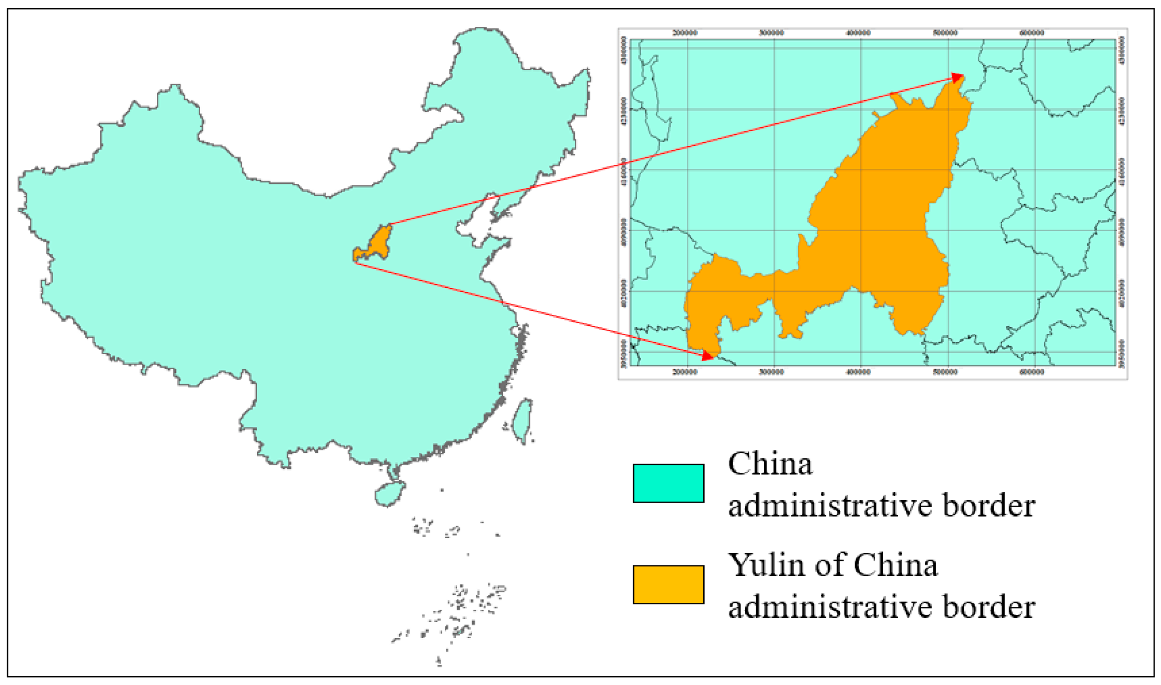
The research area is Yulin, Shaanxi Province, China. The research object is the information about the surface cracks in the sandy area. The research data are UAV images. The parameter information of UAV image data is shown in Table 1. Figure 1 shows the geographical location of Yulin, Shaanxi Province, China. Figure 2 shows four UAV image datasets.

2.1.2. Construction of the Datasets

As SVM, RF, and KNN are all supervised learning algorithms, it is necessary to build UAV image datasets for model construction. Four UAV images were cut into 50 × 50 pixel images with MATLAB, and 795 crack images and some no crack images were obtained. The background information of the UAV image refers to the land surface information mainly included in the image except for the surface cracks, which mainly include bare land and vegetation. Because background information can interfere with the classification results of machine learning, to improve classification accuracy, datasets of UAV images must be constructed reasonably.
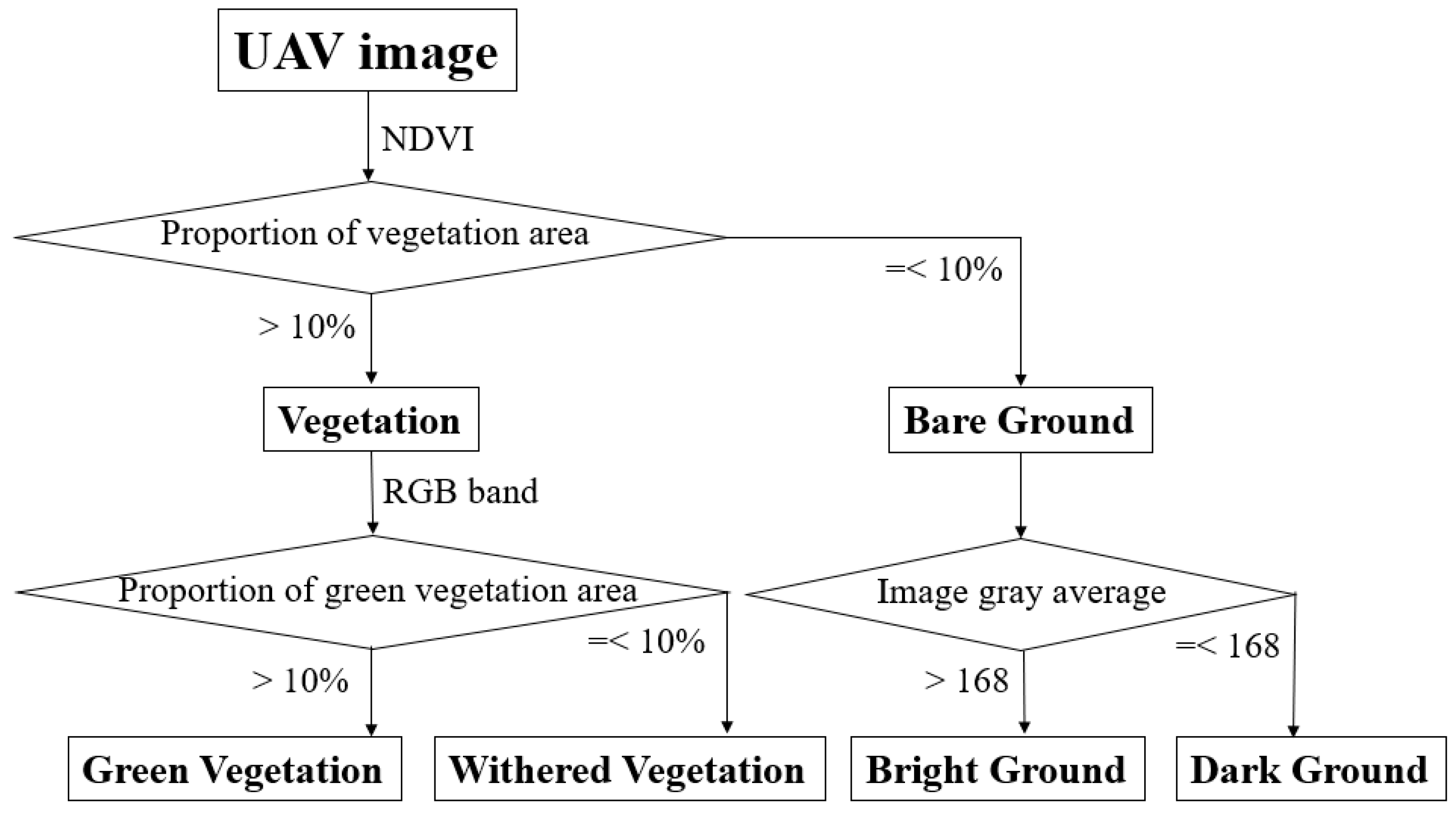
This article proposes a method based on cluster analysis [22] and the characteristics of the background information of the UAV images. The clustering method is shown in Figure 3. First, obtain the percentage of vegetation area of each image through Normalized Difference Vegetation Index (NDVI). When it exceeds 10%, divide this image into Vegetation dataset; otherwise, it is Bare Ground dataset. Then, for the images in the Vegetation dataset, obtain the percentage of the green vegetation area of each image through the RGB band. When it exceeds 10%, divide this image into the Green Vegetation dataset; otherwise, the Withered Vegetation dataset. Next, for the image of the Bare Ground dataset, convert the image into grayscale image and obtain its grayscale average value. When this value exceeds 168, divide the image into a Bright Ground dataset; otherwise, it is a Dark Ground dataset. Finally, select the same number of crack and no crack images with the same background information to construct four datasets, respectively: Green Vegetation dataset, Withered Vegetation, Bright Ground dataset, and Dark Ground dataset.
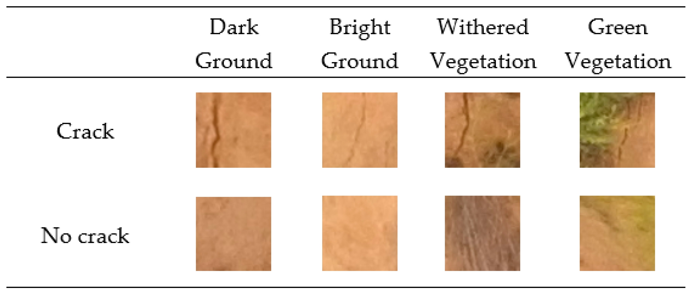
Example: Figure 4 is the classification process of one image when constructing dataset, where Figure 4a is a UAV image, Figure 4b is a vegetation image extracted through NDVI, and Figure 4c is a green vegetation image extracted through RGB. First, the percentage of vegetation area obtained through NDVI for this image is 44.2% as shown in Figure 4b, 44.2% > 10%, so this image is divided into Vegetation dataset. Then, the percentage of green vegetation area obtained through the RGB band for this image is 4.3% as shown in Figure 4c, 4.3% < 10%, so this image is divided into Withered Vegetation dataset. All other images are divided by this method, and finally four datasets are obtained: Green Vegetation dataset, Withered Vegetation, Bright Ground dataset, and Dark Ground dataset. Figure 5 is the schematic diagram of UAV images with cracks and no cracks in the four datasets.
It needs to be specifically explained that 10% and 168 both are thresholds, the 10% threshold is vegetation area percentage (vegetation area divided by image area), and the 168 threshold is image grayscale average. The first image classification according to whether its vegetation area percentage exceeds 10% threshold. Further, the second image classification according to whether its green vegetation area percentage exceeds 10% threshold for Vegetation dataset or whether its image grayscale average exceeds the 168 threshold for Bare Ground dataset. These thresholds are empirical parameters and only applicable to this research area. When using UAV images from different regions as research objects, researchers need to further determine the thresholds reasonably.
The training samples are established with cracks and no cracks as labels, and the same number of no crack images with the same background information is combined with crack images. The number of training samples for the four datasets is shown in Table 2. The features used for machine learning are all the R, G, B values of each image. As the image pixel size is 50 × 50, the total number of features values is 7500 (50 × 50 × 3).
The image background information in the D2 dataset is bright ground, containing 165 crack images and 165 no-crack images. The image background information in the D3 dataset is dark ground, containing 206 crack images and 206 no-crack images. The image background information in the D4 dataset is withered vegetation, containing 392 crack images and 392 no-crack images. The image background information in the D5 dataset is green vegetation, containing 32 crack images and 32 no-crack images. The D1 dataset is a combination of all images in the four datasets D2, D3, D4, and D5, including 795 crack images and 795 no crack images. The features of each image (7500 feature values) are used as training samples of machine learning.

2.1.3. Research Method

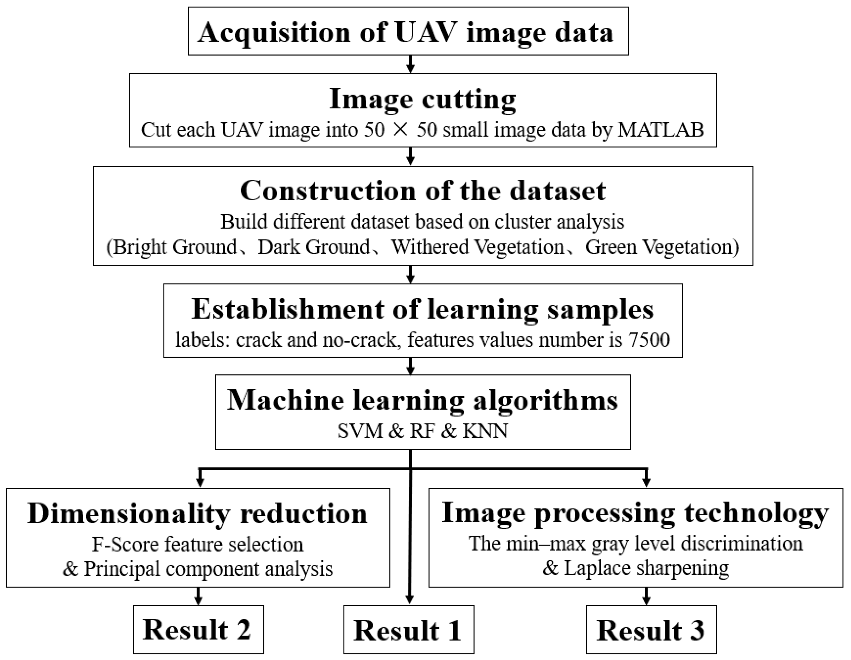
This article proposes a new identification method for surface cracks from UAV images based on machine learning in coal mining areas. As shown in Figure 6, first, the UAV image data are acquired. Second, the images were cut into 50 × 50 pixel images with MATLAB. Third, we build four types of datasets based on characteristics of the UAV image background information: bright ground, dark ground, withered vegetation, and green vegetation. Fourth, for each type of dataset, training sample is established with cracks and no cracks as labels and features values number is 7500. Finally, the best machine learning algorithms, dimensionality reduction methods, and image processing technology are selected through comparative analysis. The validation methods are leave-one-out cross-validation and permutation tests. The classification accuracy and Area Under Curve (AUC) values are evaluation indicators. Result 1 is the classification result of three machine learning algorithms, from which the best machine learning algorithm is selected. Result 2 is the classification result using two dimensionality reduction methods. Result 3 is the classification result using two image enhancement methods to process images.
The leave-one-out cross-validation is used to divide a large dataset into k small datasets. Then, k-1 is used as the training set, and the other is used as the test set. Then, select the next one as the test set, and the remaining k-1 as the training set. By analogy, the k classification accuracy is obtained and the average value is taken as the final classification accuracy of the dataset.

2.2. Machine Learning Methods

Machine learning is a common research hotspot in the field of artificial intelligence and pattern recognition. Common algorithms include support vector machine (SVM) algorithm, random forest (RF) algorithm, k-nearest neighbor (KNN) algorithm, Naïve Bayes (NB) algorithm, and deep learning (DP). It has been widely used in graphics recognition and other fields. It plays an important role in the rapid and efficient resolution of complex problems.

2.2.1. Support Vector Machine

Hoang, ND found that SVM is superior to RF and ANN machine learning algorithms in the research of asphalt pavement crack classification [23]. Wang found that the HOG + SVM (Histogram of Oriented Gradients + Support Vector Machine) method can efficiently count oil palm trees from UAV images [24]. The kernel function [25] changes in the form and parameters implicitly change the mapping from the input space to the feature space and then affect the characteristics of the feature space, ultimately changing the performance of various kernel function methods.
C-SVM is a support vector machine algorithm with parameter C as penalty function. It is a two-category classification model [26]. It is defined as the linear classifier with the largest interval in feature space. The learning strategy is margin maximization. This translates into a solution to a convex quadratic programming problem. For linearly separable cases, the C-SVM problem can be transformed into the following quadratic programming problem,
min = 1 2 w 2 + C i = 1 l ξ i
where C is a penalty parameter. The larger C is, the more the SVM punishes the incorrect classification. C is the only adjustable parameter in the C-SVM. ξ i represents a relaxation variable.   l represents the amount of variable. w represents the normal vector of the classification hyperplane in the high-dimensional space and b is the constant term. x i represents the training set.
There are two contradictory goals in C-SVM, namely, maximum margin and minimum training error, and C plays a role in regulating these two goals. The selection of parameter C is difficult. Based on C-SVM, V-SVM is proposed. V-SVM is a support vector machine algorithm with parameter V as penalty function to replace C [27]. In the case of linear separability, the V-SVM model is as follows,
min = 1 2 w 2 ρ v + 1 l i = 1 l ξ i
s . t .   y i [ w T x i + b ] ρ ξ i ,   i = 1 , 2 , , l ,   ρ 0 ,   ξ i 0 ,   i = 1 , 2 , , l ,
where l is the number of training sample points. The parameter v can be used to control the number and error of support vectors. In addition, it is also easier to choose. Parameter ρ represents two types of points (classes −1 and +1) that are separated by an interval of 2 ρ w .

2.2.2. Random Forest

Random forest (RF) is a classifier containing multiple decision trees in machine learning. Its output category is determined by the mode of the categories output by individual trees [28]. Quanlong F. has achieved good results using the UAV images for Urban Vegetation Mapping through random forest [29]. Su J. has achieved good monitoring results by random forest algorithm to monitor Wheat yellow rust from multispectral UAV aerial imagery [30].
Random forest [31] uses bootstrap resampling technology to randomly extract k samples from the original training sample set N to generate a new training sample set and then generates k based on the self-service sample set. Each classification tree forms a random forest, and the classification results of the new data are determined by how many points the classification tree votes. In essence it is an improvement on the decision tree algorithm. Multiple decision trees are merged together. The establishment of each tree depends on an independent sample. Each tree in the forest has the same distribution. The classification error depends on the classification ability of each tree and the correlation between them.
Random forest has three main hyperparameter adjustments: node size, number of trees, and number of predictor samples. A reasonable selection of the number of trees can effectively improve the accuracy of classification.

2.2.3. K-Nearest Neighbors

The core idea of k-nearest neighbor is that if most of the k-nearest-neighbors of a sample in the feature space belong to a certain category, then the sample also belongs to this category and has the characteristics of this category [32]. In determining the classification decision, the method only determines the category to which the sample to be classified belongs according to the category of the nearest sample or samples. The KNN method is only related to a very small number of adjacent samples when making category decisions. The KNN method mainly depends on the limited neighboring samples, rather than the method of discriminating the class domain. The KNN method is more suitable than other methods for the set of sample domains that have many intersections or overlaps [33]. Liu K. has achieved good results that estimating forest structural attributes using UAV-LiDAR data by K-Nearest Neighbors [34]. The three elements of the KNN algorithm are distance measurement, k-value selection, and classification decision rules.

2.3. Dimensionality Reduction Method

Dimensionality is the number of feature vectors in the image. More than three feature vectors perpendicular to each other represents a high-dimensional space that cannot be visualized. When the dimension is higher, the amount of information contained is larger, and the classification difficulty of the machine learning algorithm is also greater. When the dimension exceeds a certain value, the curse of dimensionality occurs [35]. At this time, dimensionality reduction is needed to achieve the best classification effect.

2.3.1. F-Score Feature Selection

Feature selection selects the features that are most effective for classification and recognition from among many features to achieve compression of the feature space dimension. The F-score is a method for measuring the ability of features to be distinguished between two categories [36]. This method can achieve the most effective feature selection, and the detailed description is as follows.
The training sample set xk ∈ Rm, k = 1, 2,…, n where n+ and n− are the number of positive and negative samples, respectively. The F-score of the i-th feature of the training sample is defined as
F i = ( x ¯ i ( + ) x ¯ i ) 2 + ( x ¯ i ( ) x ¯ i ) 2 1 n + 1 k = 1 n + ( x ¯ k i ( + ) x ¯ i ( + ) ) 2 + 1 n 1 k = 1 n ( x ¯ k i ( ) x ¯ i ( ) ) 2
where x ¯ i ,   x ¯ i ( + ) , and x ¯ i ( ) are the average value of the i-th feature over the entire dataset, the average value on the positive type dataset, and the negative type dataset, respectively; x ¯ k i ( + ) is the eigenvalue of the i-th feature of the k-th positive sample point; and x ¯ k i ( ) is the k-th negative sample point.

2.3.2. Principal Component Analysis

Principal component analysis (PCA) is a dimensionality reduction method often used in image processing [37]. The steps are as follows.
First, input the sample set D = {x1, x2, …, xm} and map it to the low-dimensional (k-dimensional) space dimension. Second, transform the samples in X to the standard normal distribution N ~ (0,1). Third, find the covariance matrix XTX∈Rm*m and solve the eigenvalues and eigenvectors of the covariance matrix, X T X = V V 1 . Fourth, find the maximum k eigenvalues and the corresponding eigenvectors and record them as ( ω 1 , ω 2 , ω 3 ω k ) and output them as W = { ω 1 , ω 2 , ω 3 ω k }.

2.4. Image Processing Technology

Image enhancement is a common image processing method. It can emphasize the local features of an image [23]. According to the difference in the nature of the enhanced image, it can be divided into two types: one is image gray enhancement, the image is a grayscale image after enhancement, and the other is image color enhancement, the image is a color image after enhancement. This article selects two representative image enhancement methods for research, the min–max gray level discrimination and laplace sharpening.

2.4.1. The Min–Max Gray Level Discrimination (M2GLD)

Hoang [38] proposed a method for min–max gray level discrimination for image gray enhancement, hereinafter referred to as M2GLD. Let I0(m,n) be the gray value of a pixel at the coordinate (m,n), and I0(m,n) is transformed using the following formulas,
I A ( m , n ) = m i n ( I 0 m a x ,   R A )   i f   I 0 ( m , n ) > I 0 m i n   + τ · ( I 0 m a x I 0 m i n   )
I A ( m , n ) = m a x ( I 0 m i n ,   R A 1 )   i f   I 0 ( m , n )   I 0 m i n   + τ · ( I 0 m a x I 0 m i n   )
where IA(m,n) represents the adjusted gray intensity of the pixel at position (m,n). RA denotes the adjusting ratio. I 0 m a x and I 0 m i n   represent the maximum and minimum values of the gray intensity of the original image, respectively. τ is a margin parameter.
The M2GLD method aims at discriminating the gray intensity of potential crack and noncrack pixels. Hence, after being processed, the crack pixels become darker and the noncrack pixels tend to be lighter. In this article, referring to Nhat-Duc Hoang [38], the two parameters RA and τ are selected as 1.5 and 0.1.

2.4.2. Laplace Sharpening

The Laplace operator [39] is an edge detection operator. The effect of this operator on f(x,y) is
2 f = f 2 x 2 + f 2 y 2
From the sharpening formula of the one-dimensional signal, the sharpening formula of the two-dimensional digital image is
g ( m , n ) = f ( m , n ) + α [ 2 f ( m , n ) ]
In digital image processing, f 2 x 2 and f 2 y 2 can be expressed as a differential equation as
f 2 x 2 = f ( m + 1 , n ) + f ( m 1 , n ) 2 f ( m , n )
f 2 y 2 = f ( m , n + 1 ) + f ( m , n 1 ) 2 f ( m , n )
By adding Equations (10) and (11) into g (m, n), the Laplacian sharpening expression is
g ( m , n ) = ( 1 + 4 α ) f ( m , n ) α [ f ( m , n + 1 ) + f ( m , n 1 ) + f ( m + 1 , n ) + f ( m 1 , n ) ]
where α is the sharpening intensity coefficient. The larger the α, the stronger the sharpening degree, and the larger the “overshoot” corresponding to the figure.

3. Results

3.1. Comparison of Machine Learning Algorithms

3.1.1. Penalty Function Selection of SVM

Table 3 shows the classification results of UAV image surface cracks by SVM with two kernel functions: C-SVM and V-SVM. The classification accuracy and AUC values are used as evaluation indicators. Table 3 shows that the classification accuracy and AUC value of V-SVM are higher than those of C-SVM, which has a better classification effect.

3.1.2. Tree Number Selection of RF

The number of trees is an important parameter of the RF. This article uses 100, 200, 300, 400, and 500 as the quantitative parameters of the tree.
Table 4 shows the classification results of UAV image surface cracks by RF. The classification accuracy and AUC values are used as evaluation indicators. From Table 4, we find that when the number of RF trees is between 100 and 500, the classification accuracy of the RF has little difference, and it is relatively optimal when the number of RF trees selected is 300 for a comprehensive comparison.

3.1.3. K-Value Selection of KNN

K-value selection is one of the elements of the KNN. Cross-validation is usually used to select a suitable k value. This article uses 3, 6, 9, 12, and 15 as k-value parameters for research.
Table 5 shows the classification results of UAV image surface cracks by KNN. The classification accuracy and AUC values are used as evaluation indicators. From Table 5, we find that when the k value of the KNN is between 3 and 15, the classification accuracy of the KNN is not significantly different, and it is relatively optimal when the k value of the KNN is 9 for a comprehensive comparison.

3.1.4. Optimization of SVM & RF & KNN

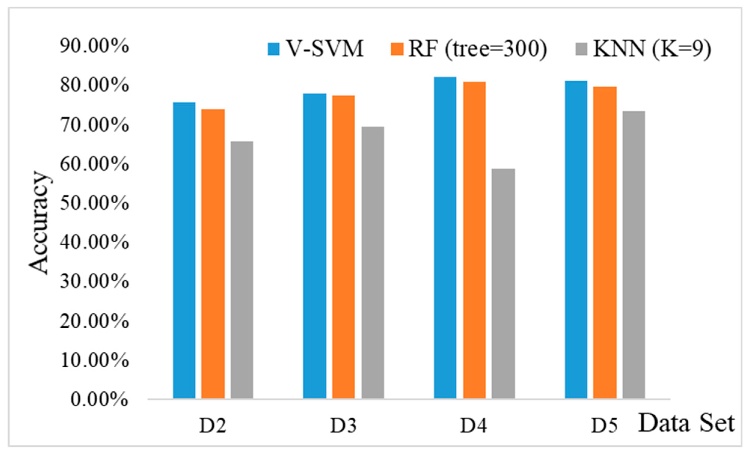
The methods with the best parameters in SVM, RF, and KNN are selected to compare the machine learning algorithms. SVM selects V-SVM, the number of RF tree selections is 300, and the K value of KNN selection is 9. The comparison of the prediction results of the three machine learning algorithms of SVM, RF, and KNN is shown in Table 6 and Figure 7. V-SVM has the best classification accuracy.

3.2. Comparison of Dimensionality Reduction Methods

Dimensionality is the number of feature vectors in the image. More than three feature vectors are perpendicular to each other. It is a high-dimensional space that cannot be visualized. When the dimension is higher, the amount of information contained is larger, and the classification difficulty of the machine learning algorithm is also greater. When the dimension exceeds a certain value, the phenomenon of the dimension disaster (curse of dimensionality) will occur [35]. At this time, dimensionality reduction is needed to achieve the best classification effect.

3.2.1. F-Score Feature Selection

The parameter selection of the F-score is 0.1:0.1:1, which means that according to the weight/F value, the first 0.1 features are selected first, and then 0.1 is used as the step size, and the features are selected gradually to 1 (100%). V-SVM is used as the machine learning algorithm. Four datasets, D2, D3, D4, and D5, are used as the research objects. The classification results are shown in Figure 8, where the left figure is a schematic diagram of the change in accuracy in the case of different feature selections. The figure on the right is the ROC curve and its AUC value. As seen in Figure 8, when full feature selection is performed on the image, the classification accuracy and AUC value are the largest, which has a better classification effect.

3.2.2. Principal Component Analysis

Principal component analysis (PCA) is a commonly used method of dimensionality reduction. This research compares the classification results with 95% dimensionality reduction and no dimensionality reduction. V-SVM is used as the machine learning algorithm. Four datasets, D2, D3, D4, and D5, are used as the research objects. The classification accuracy and AUC values are used as evaluation indicators. Table 7 shows the results of the surface crack classification in UAV images using PCA to reduce the dimensions to 95% of the original variance and no dimensionality reduction. It can be seen from Table 7 that when PCA is used to reduce the dimensions to 95% of the original variance, its classification accuracy and AUC value are greater, which has a better classification effect.

3.3. Comparison of Image Processing Technologies

3.3.1. The Min–Max Gray Level Discrimination (M2GLD)

M2GLD is an image gray enhancement image processing technology. Table 8 is a schematic diagram of the effect of the image after M2GLD and the original image, where A represents the original image and B represents the image after M2GLD. V-SVM is used as the machine learning algorithm. Four datasets, D2, D3, D4, and D5, are used as the research objects. The classification accuracy and AUC values are used as evaluation indicators. Table 9 shows the results of the surface crack classification in UAV images using M2GLD and No-M2GLD. It can be seen from Table 9 that when M2GLD is used to enhance the grayscale of an image, its classification accuracy and AUC value are smaller, which has a worse classification effect.

3.3.2. Laplace Sharpening

Laplace sharpening is an image color enhancement image processing technology. Table 10 is a schematic diagram of the effect of the image after Laplace sharpening and the original image, where A represents the original image and B represents the image after Laplace sharpening. V-SVM is used as the machine learning algorithm. Four datasets, D2, D3, D4, and D5, are used as the research objects. The classification accuracy and AUC values are used as evaluation indicators. Table 11 shows the results of the surface crack classification in UAV images using Laplace sharpening and no Laplace sharpening. It can be seen from Table 11 that when Laplace sharpening is used to enhance the color of an image, its classification accuracy and AUC value are greater, which has a better classification effect.

3.4. Comparison of Cluster Analysis Results

In view of the fact that background information will interfere with the classification results of machine learning algorithms, based on the idea of cluster analysis and characteristics of the background information of the UAV image, this article divides the UAV image data into four types of datasets, namely, bright ground, dark ground, withered vegetation, and green vegetation. V-SVM is used as the machine learning algorithm. Four datasets, D2, D3, D4, and D5, are used as the research objects. The images are processed by Laplace sharpening image color enhancement processing. PCA is used to reduce the dimensions to 95% of the original variance for all features. The classification accuracy and AUC values are used as evaluation indicators. The final classification results are shown in Table 12.
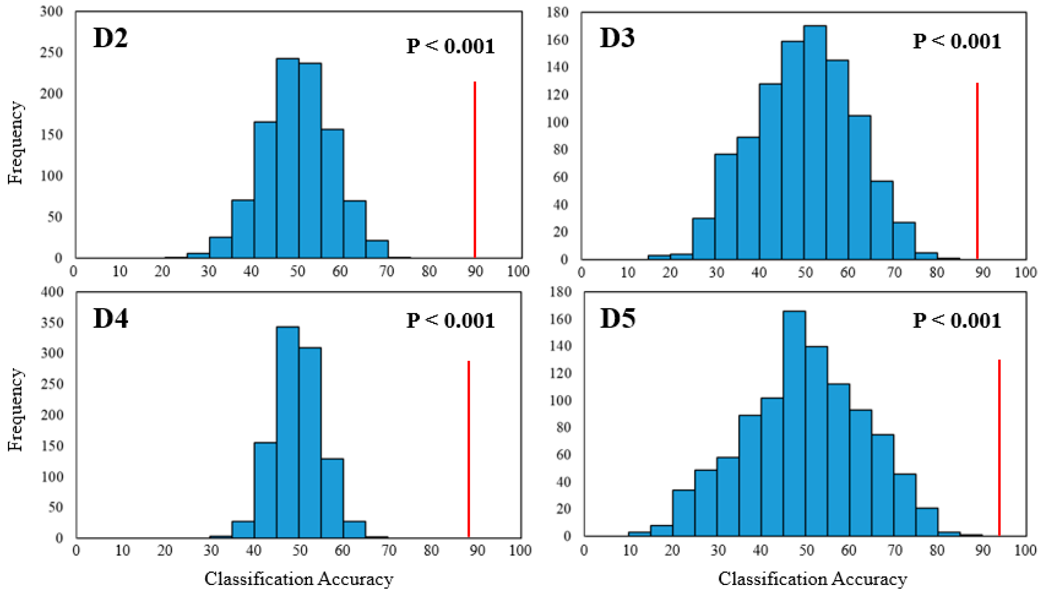
Statistically significant p-values are obtained by permutation tests. The permutation test is a method proposed by Fisher that is computationally intensive, uses a random arrangement of sample data to perform statistical inference, and is widely used in the field of machine learning. The specific use is similar to bootstrap methods by sequentially replacing samples, recalculating statistical tests, constructing empirical distributions, and then inferring the p-value based on this. Assume N replacement tests are performed, and the classification accuracy rate obtained by n replacement tests is higher than the true accuracy rate, then p-value = n/N. When the classification accuracy rate obtained without the replacement test is higher than the true accuracy rate, it is usually recorded as p-value <1/N. The smaller the p-value is, the more significant the difference. In this article, N = 1000 permutation tests are performed on the four datasets. As shown in Figure 9, the blue histogram represents the statistical distribution of classification accuracy for 1000 replacement tests, and the red straight line represents the true accuracy.
As shown in Table 12 and Figure 9, the p-values of the four datasets are <0.001. This indicates that the classification effect of machine learning has strong statistical significance. The classification accuracy of bright ground reaches 89.70%, dark ground reaches 88.35%, winter vegetation reaches 88.65%, green vegetation reaches 93.75%, and the overall classification accuracy reaches 88.99%.
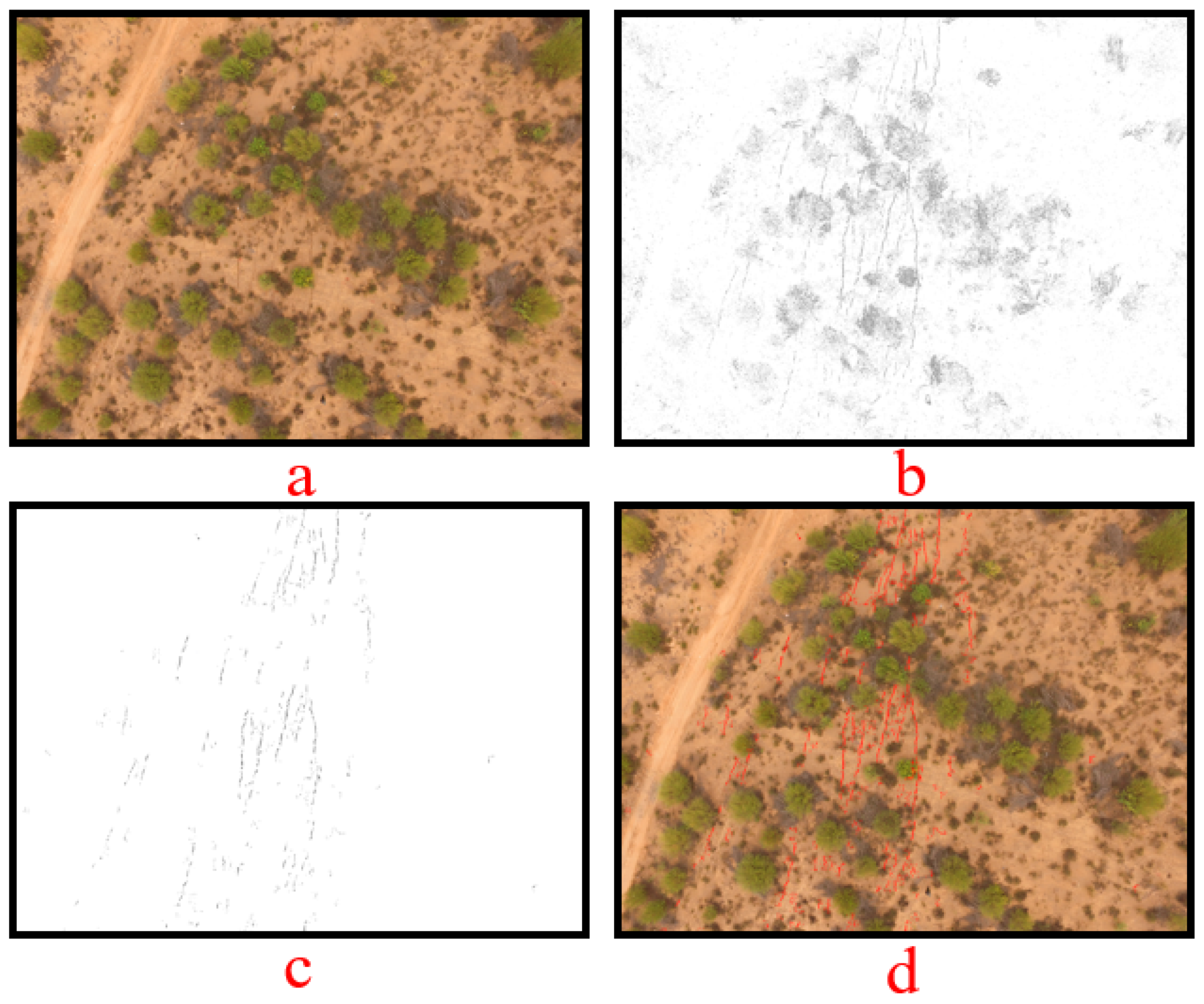
The method proposed in this article is used to identify whether the UAV image has cracks. The edge segmentation method is used to extract cracks from the UAV image with cracks, and the results are processed by the opening operation. The processing becomes a white background from the UAV image with no cracks. Finally, each processed image is joined according to the serial number of the image cutting. The final schematic diagram of the crack extraction effect in the UAV image is shown in Figure 10, where Figure 10a represents the original UAV image, Figure 10b represents the schematic diagram of the crack extraction effect by edge segmentation for the original UAV image, Figure 10c represents the schematic diagram of the crack extraction effect by edge segmentation for the UAV image after the method mentioned in this article, and Figure 10d represents the comparison of the final schematic diagram of the crack extraction effect in the UAV image and original UAV image. Figure 10 shows that the effect in Figure 10c is better than the effect in Figure 10b, and the method proposed in this article can extract crack information from UAV images well.

4. Discussion

4.1. Machine Learning Methods

In the SVM machine learning algorithm, when the parameter penalty function C of C-SVM tends to infinity, it means that samples with classification errors are not allowed to exist, and it easily causes hard-margin SVM overfitting. When C approaches 0, it means no longer focus on whether the classification is correct; only the interval needs to be maximized, which easily leads to underfitting of the algorithm. V-SVM uses a new parameter V instead of C, which can be used to control the number and error of support vectors and is relatively easy to choose. Therefore, better classification results are achieved.
In the RF machine learning algorithm, the classification effect improves correspondingly with the increase in the tree within a certain range. When it reaches a certain number, it will be balanced. However, when the number of trees is too large, it will cause overfitting. Instead, the classification accuracy of the random forest is reduced. Therefore, the final selection number of trees is 300 through comparative analysis.
In the KNN machine learning algorithm, the classification effect improves as the k value decreases in a certain range. However, when the k value is too low, it will cause overfitting. Therefore, this article finally chooses the k value of 9 through comparative analysis.
Among the three machine learning algorithms for surface crack extraction in mining areas, SVM is superior to RF and KNN. It has the best classification effect, which is consistent with the conclusions of Hoang. in research on road crack extraction [23].

4.2. Dimensionality Reduction Method

In the F-score feature selection, as the UAV images have been cut, the information contained in each image has been sufficiently simplified. Therefore, full feature selection has been adopted to achieve better classification results. When PCA is used to reduce the dimensions to 95% of the original variance, its classification accuracy and AUC value are greater, which has a better classification effect. This is consistent with the conclusions of Chen W. in research on face detection and recognition using PCA for dimensionality reduction has a better detection success rate [40].

4.3. Image Processing Technology

Before performing machine learning, images are usually preprocessed first, among which image enhancement methods are widely used. In this article, the min–max gray level discrimination (M2GLD) and Laplace sharpening image enhancement methods are selected for research. M2GLD is an image gray enhancement method that has no effect on the classification accuracy of surface cracks in mining areas. This may be because when the color image is converted into a gray image to enhance the crack information, the background interference information is also enhanced, resulting in worse classification results. Laplace sharpening is an image color enhancement method that can effectively enhance the crack information of the land in the mining area and has achieved a good classification effect. Jijun W. uses the four-neighbor laplace sharpening to enhance image detail information and obtain more effective results [41]. This is consistent with our results using laplace sharpening to enhance the image crack information and obtain higher classification accuracy.

4.4. Cluster Analysis Results

UAV remote sensing technology plays an important role in land reclamation in mining areas and has the characteristics of low cost and high efficiency. Machine learning has been widely used in the field of pattern recognition. This article proposes a new identification method for surface cracks from UAV images based on machine learning in coal mining areas. This method first cuts the drone images to simplify the surface information contained in each image and then uses the idea of cluster analysis to differentiate the background information of the images. Clustering is performed twice so that images with similar background information are combined to build datasets: bright ground, dark ground, withered vegetation, and green vegetation. Therefore, this method can effectively reduce the interference of background information on the classification results. The overall accuracy is improved to 88.99%.
5. Conclusions

This article proposes a new identification method for surface cracks from UAV images based on machine learning in coal mining areas. The cluster analysis is used to construct different datasets based on the background information of the image. Through dimensionality reduction methods and image processing technologies, three types of SVM, RF, and KNN are compared. The following four conclusions are made.
  • In the surface crack recognition of UAV images, the accuracy of SVM is better than the RF and KNN.
  • Image color enhancement can improve the accuracy of machine learning, but image gray enhancement cannot.
  • Reasonable use of dimensionality reduction methods can improve the accuracy of machine learning
  • By using the V-SVM machine learning algorithm, PCA to reduce the full features to 95% of the original variance, and image color enhancement by Laplace sharpening, the overall accuracy could reach 88.99%.
The method provided in this article could effectively identify and extract ground cracks. It would provide data support for further research on the crack information such as the length, width, direction, and crack rate of the surface cracks and the development regularity.

Author Contributions

Conceptualization, F.Z. and Z.H.; methodology, F.Z. and Y.F.; software, F.Z.; formal analysis, K.Y.; investigation, Y.F.; resources, K.Y.; data curation, F.Z.; writing—original draft preparation, F.Z.; writing—review and editing, Z.H.; project administration, Z.F.; funding acquisition, Q.W. All authors have read and agreed to the published version of the manuscript.

Funding

This research was funded by the Research and Demonstration of Key Technology for Water Resources Protection and Utilization and Ecological Reconstruction in Coal Mining area of Northern Shaanxi, grant number is 2018SMHKJ-A-J-03.

Acknowledgments

We thank Sijia Wang from Tianjin Medical University for the inspiration to explore the identification method for surface cracks from UAV images based on machine learning.

Conflicts of Interest

The authors declare no conflict of interest.

References

  1. Xu, L.; Li, S.; Cao, X.; Somerville, I.D.; Cao, H. Holocene intracontinental deformation of the northern north china plain: Evidence of tectonic ground fissures. J. Asian Earth Sci. 2016, 119, 49–64. [Google Scholar] [CrossRef]
  2. Li, Y.; Yang, J.; Hu, X. Origin of ground fissures in the Shanxi Graben System, Northern China. Eng. Geol. 2000, 55, 267–275. [Google Scholar] [CrossRef]
  3. Wang, W.; Yang, Z.; Kong, J.; Cheng, D.; Duan, L.; Wang, Z. Ecological impacts induced by groundwater and their thresholds in the arid areas in Northwest China. Environ. Eng. Manag. J. 2013, 12, 1497–1507. [Google Scholar] [CrossRef]
  4. Youssef, A.M.; Sabtan, A.A.; Maerz, N.H.; Zabramawi, Y.A. Earth fissures in wadi najran, kingdom of saudi arabia. Nat. Hazards 2014, 71, 2013–2027. [Google Scholar] [CrossRef]
  5. Stumpf, A.; Malet, J.P.; Kerle, N.; Niethammer, U.; Rothmund, S. Image-based mapping of surface fissures for the investigation of landslide dynamics. Geomorphology 2013, 186, 12–27. [Google Scholar] [CrossRef] [Green Version]
  6. Kasai, M.; Ikeda, M.; Asahina, T.; Fujisawa, K. LiDAR-derived DEM evaluation of deep-seated landslides in a steep and rocky region of Japan. Geomorphology 2009, 113, 57–69. [Google Scholar] [CrossRef]
  7. Glenn, N.F.; Streutker, D.R.; Chadwick, D.J.; Thackray, G.D.; Dorsch, S.J. Analysis of LiDAR-derived topographic information for characterizing and differentiating landslide morphology and activity. Geomorphology 2006, 73, 131–148. [Google Scholar] [CrossRef]
  8. Shruthi, R.B.V.; Kerle, N.; Jetten, V. Object-based gully feature extraction using high spatial resolution imagery. Geomorphology 2011, 134, 260–268. [Google Scholar] [CrossRef]
  9. Peng, J.; Qiao, J.; Leng, Y.; Wang, F.; Xue, S. Distribution and mechanism of the ground fissures in wei river basin, the origin of the silk road. Environ. Earth Sci. 2016, 75, 718. [Google Scholar] [CrossRef]
  10. Zheng, X.; Xiao, C. Typical applications of airborne lidar technolagy in geological investigation. Int. Arch. Photogramm. Remote Sens. Spat. Inf. Sci. 2018, 42, 3. [Google Scholar] [CrossRef] [Green Version]
  11. Mohan, A.; Poobal, S. Crack detection using image processing: A critical review and analysis. Alex. Eng. J. 2018, 57, 787–798. [Google Scholar] [CrossRef]
  12. Nex, F.; Remondino, F. Uav for 3d mapping applications: A review. Appl. Geomat. 2014, 6, 1–15. [Google Scholar] [CrossRef]
  13. Pádua, L.; Vanko, J.; Hruka, J.; Adao, T.; Sousa, J.J.; Peres, E.; Morais, R. UAS, sensors, and data processing in agroforestry: A review towards practical applications. Int. J. Remote Sens. 2017, 38, 2349–2391. [Google Scholar] [CrossRef]
  14. Maragos, P.; Sofou, A.; Stamou, G.B.; Tzouvaras, V.; Papatheodorou, E.; Stamou, G.P. Image analysis of soil micromorphology: Feature extraction, segmentation, and quality inference. EURASIP J. Adv. Signal Process. 2004, 2004, 902–912. [Google Scholar] [CrossRef] [Green Version]
  15. Lindi, J.Q. A review of techniques for extracting linear features from imagery. Photogramm. Eng. Remote Sens. 2004, 70, 1383–1392. [Google Scholar] [CrossRef] [Green Version]
  16. Papari, G.; Petkov, N. Edge and line oriented contour detection: State of the art. Image Vis. Comput. 2011, 29, 79–103. [Google Scholar] [CrossRef]
  17. Chambon, S.; Gourraud, C.; Moliard, J.M.; Nicolle, P. Road Crack Extrction with Adapted Filtering and Markov Model-Based Segmentation Introduction and Validation; Insticc-Inst Syst Technologies Information Control & Communication: Setubal, Portugal, 2010. [Google Scholar]
  18. Carrio, A.; Sampedro, C.; Rodriguez-Ramos, A.; Campoy, P. A review of deep learning methods and applications for unmanned aerial vehicles. J. Sens. 2017. [Google Scholar] [CrossRef]
  19. Fei, Y.; Wang, K.C.P.; Zhang, A.; Chen, C.; Li, J.Q.; Liu, Y.; Yang, G.; Li, B. Pixel-level cracking detection on 3d asphalt pavement images through deep-learning-based cracknet-v. IEEE Trans. Intell. Transp. Syst. 2020, 21, 273–284. [Google Scholar] [CrossRef]
  20. Ammour, N.; Alhichri, H.; Bazi, Y.; Benjdira, B.; Alajlan, N.; Zuair, M. Deep learning approach for car detection in UAV imagery. Remote Sens. 2017, 9, 312. [Google Scholar] [CrossRef] [Green Version]
  21. Zeggada, A.; Melgani, F.; Bazi, Y. A deep learning approach to uav image multilabeling. IEEE Geoence Remote Sens. Lett. 2017, 14, 694–698. [Google Scholar] [CrossRef]
  22. Everitt, B. Cluster analysis. Qual. Quant. 1980, 14, 75–100. [Google Scholar] [CrossRef]
  23. Hoang, N.D.; Nguyen, Q.L. A novel method for asphalt pavement crack classification based on image processing and machine learning. Eng. Comput. 2019. [Google Scholar] [CrossRef]
  24. Wang, Y.; Zhu, X.; Wu, B. Automatic detection of individual oil palm trees from uav images using hog features and an svm classifier. Int. J. Remote Sens. 2019, 40, 7356–7370. [Google Scholar] [CrossRef]
  25. Mercer, J. Functions of positive and negative type and their connection with the theory of integral equations. Philos. Trans. Roy. Soc. Lond. 1909, 559, 415–446. [Google Scholar] [CrossRef]
  26. Zhang, L.; Zhang, B. Relationship between support vector set and kernel functions in svm. J. Comput. Sci. Technol. 2002, 17, 549–555. [Google Scholar] [CrossRef]
  27. Wang, X.; Wu, S.; Li, Q.; Wang, X. v-SVM for transient stability assessment in power systems. Autonomous Decentralized Systems. In Proceedings of the ISADS 2005, Chengdu, China, 4–8 April 2005. [Google Scholar] [CrossRef]
  28. Breiman, L. Random forests. Mach. Learn. 2001, 45, 5–32. [Google Scholar] [CrossRef] [Green Version]
  29. Quanlong, F.; Jiantao, L.; Jianhua, G. Uav remote sensing for urban vegetation mapping using random forest and texture analysis. Remote Sens. 2015, 7, 1074–1094. [Google Scholar] [CrossRef] [Green Version]
  30. Su, J.; Liu, C.; Coombes, M.; Hu, X.; Wang, C.; Xu, X.; Li, Q.; Guo, L.; Chen, W.H. Wheat yellow rust monitoring by learning from multispectral uav aerial imagery. Comput. Electron. Agric. 2018, 155, 157–166. [Google Scholar] [CrossRef]
  31. Waske, B.; van der Linden, S.; Oldenburg, C.; Jakimow, B.; Rabe, A.; Hostert, P. Imagerf—A user-oriented implementation for remote sensing image analysis with random forests. Environ. Model. Softw. 2012, 35, 192–193. [Google Scholar] [CrossRef]
  32. Pan, J.; Manocha, D. Bi-level locality sensitive hashing for k-nearest neighbor computation. In Proceedings of the 2012 IEEE 28th International Conference on Data Engineering, Washington, DC, USA, 1–5 April 2012. [Google Scholar] [CrossRef]
  33. Sismanis, N.; Pitsianis, N.; Sun, X. Parallel Search of k-Nearest Neighbors with Synchronous Operations. IEEE High Perform. Extrem. Comput. 2012. [Google Scholar] [CrossRef]
  34. Liu, K.; Shen, X.; Cao, L.; Wang, G.; Cao, F. Estimating forest structural attributes using uav-lidar data in ginkgo plantations. ISPRS J. Photogramm. Remote Sens. 2018, 146, 465–482. [Google Scholar] [CrossRef]
  35. Chan, T.-H.H.; Jiang, S.H.-C. Reducing curse of dimensionality: Improved ptas for tsp (with neighborhoods) in doubling metrics. ACM Trans. Algorithms 2018, 14, 1–18. [Google Scholar] [CrossRef]
  36. Tao, P.; Yi, H.; Wei, C.; Ge, L.Y.; Xu, L. A method based on weighted F-score and SVM for feature selection. In Proceedings of the 2013 25th Control and Decision Conference (CCDC), Guiyang, China, 25–27 May 2013. [Google Scholar] [CrossRef]
  37. Hervé, A.; Williams, L.J. Principal component analysis. Wiley Interdiscip. Rev. Comput. Stat. 2018, 2, 433–459. [Google Scholar] [CrossRef]
  38. Hoang, N.D. Detection of surface crack in building structures using image processing technique with an improved Otsu method for image thresholding. Adv. Civil. Eng. 2018, 2018, 3924120. [Google Scholar] [CrossRef] [Green Version]
  39. Wang, X.Y.; Niu, P.P.; Yang, H.Y.; Chen, L.L. Affine invariant image watermarking using intensity probability density-based Harris laplace detector. J. Vis. Commun. Image Represent. 2012, 23, 892–907. [Google Scholar] [CrossRef]
  40. Chen, W. Application of Multi-Scale Principal Component Analysis and SVM to the Motor Fault Diagnosis. In Proceedings of the International Forum on Information Technology & Applications, Chengdu, China, 15–17 May 2009. [Google Scholar] [CrossRef]
  41. Jijun, W. An uav image matching method based on sift and laplace image sharpening. Beijing Surv. Mapp. 2019. [Google Scholar] [CrossRef]
Figure 1. Geographical location of Yulin, Shaanxi Province, China.
Remotesensing 12 01571 g001
Figure 2. Unmanned aerial vehicle (UAV) image data.
Remotesensing 12 01571 g002
Figure 3. Flowchart of dataset construction.
Remotesensing 12 01571 g003
Figure 4. The classification process of one image when constructing dataset (a) is a UAV image, (b) is a vegetation image extracted through NDVI, and (c) is a green vegetation image extracted through RGB).
Remotesensing 12 01571 g004
Figure 5. Schematic diagram of the UAV images with cracks and no cracks in the four datasets.
Remotesensing 12 01571 g005
Figure 6. Flowchart of a new identification method for surface cracks from UAV images based on machine learning in coal mining areas.
Remotesensing 12 01571 g006
Figure 7. Comparison of the prediction results of three machine learning algorithms.
Remotesensing 12 01571 g007
Figure 8. Comparison of F-score feature selection results.
Remotesensing 12 01571 g008
Figure 9. The results of the permutation test (N = 1000).
Remotesensing 12 01571 g009
Figure 10. Final schematic diagram of the crack extraction effect in the UAV image. (a) is the original UAV image, (b) is thethe schematic diagram of the crack extraction effect by edge segmentation for the original UAV image, (c) is the schematic diagram of the crack extraction effect by edge segmentation for the UAV image after the method mentioned in this article, and (d) is the comparison of the final schematic diagram of the crack extraction effect in the UAV image and original UAV image.
Remotesensing 12 01571 g010
Table 1. UAV image data parameter information.
ParametersValue
Data typeMultispectral image
Flight dateJune 25, 2019
Flight height50 m
UAV modelM210RTK
Camera modelMS600pro
Focal length6 mm
Band range450 nm, 555 nm, 660 nm, 710 nm, 840 nm and 940 nm
Ground spatial resolution (GSD)3.125 cm
Table 2. The number of training samples for the four datasets.
DatasetBackground InformationNumber of Training Samples
CrackNo CrackTotal
D1ALL7957951590
D2Bright Ground165165330
D3Dark Ground206206412
D4Withered Vegetation392392784
D5Green Vegetation323264
Table 3. Prediction performance of C-SVM and V-SVM for the testing dataset.
Type C-SVMV-SVM
DatasetNumber of Training SamplesNumber of Correct ClassificationsAccuracyAUCNumber of Correct ClassificationsAccuracyAUC
D11590107667.67%0.7219120475.72%0.8022
D233023972.42%0.759725777.88%0.8172
D341231175.49%0.771633882.04%0.8855
D478460877.55%0.830863681.12%0.8379
D5645484.38%0.90115789.06%0.9619
Table 4. Prediction performance of random forest (RF) for the testing dataset.
Number of Trees100200300400500
DatasetAccuracy
D270.91%71.52%73.94%73.64%73.64%
D376.46%76.94%77.43%77.43%76.94%
D479.34%80.36%80.99%80.87%80.87%
D576.56%78.13%79.69%78.13%79.69%
Mean75.82%76.74%78.01%77.52%77.79%
Table 5. Prediction performance of K-nearest neighbor (KNN) for the testing dataset.
Value of k3691215
DatasetAccuracy
D263.64%64.55%65.76%65.76%65.15%
D367.50%67.00%69.50%69.00%68.50%
D457.50%56.17%58.83%57.00%58.00%
D571.88%62.50%73.44%71.88%73.44%
Mean65.13%62.55%66.88%65.91%66.27%
Table 6. Comparison of prediction performance of support vector machine (SVM), RF, and KNN.
TypeV-SVMRF (Tree = 300)KNN (K = 9)
DatasetAccuracy
D275.72%73.94%65.76%
D377.88%77.43%69.50%
D482.04%80.99%58.83%
D581.12%79.69%73.44%
Mean79.19%78.01%66.88%
Table 7. Comparison of the results of the surface crack classification using PCA to reduce the dimensions to 95% of the original variance and no dimensionality reduction.
Type No Dimensionality ReductionDimensionality Reduction 95%
DatasetNumber of Training SamplesNumber of Correct ClassificationsAccuracyAUCNumber of Correct ClassificationsAccuracyAUC
D233027382.73%0.857228486.06%0.9619
D341233882.04%0.837934884.47%0.9251
D478465683.67%0.885567485.97%0.9464
D5645789.06%0.96195992.19%0.9671
Table 8. Schematic diagram of the effect of the image after M2GLD and original image.
Dark GroundBright Ground Withered VegetationGreen Vegetation
ABABABAB
Crack Remotesensing 12 01571 i001 Remotesensing 12 01571 i002 Remotesensing 12 01571 i003 Remotesensing 12 01571 i004 Remotesensing 12 01571 i005 Remotesensing 12 01571 i006 Remotesensing 12 01571 i007 Remotesensing 12 01571 i008
No crack Remotesensing 12 01571 i009 Remotesensing 12 01571 i010 Remotesensing 12 01571 i011 Remotesensing 12 01571 i012 Remotesensing 12 01571 i013 Remotesensing 12 01571 i014 Remotesensing 12 01571 i015 Remotesensing 12 01571 i016
Table 9. The results of the surface crack classification in UAV images using M2GLD and no M2GLD.
Type M2GLDNo M2GLD
DatasetNumber of Training SamplesNumber of Correct ClassificationsAccuracyAUCNumber of Correct ClassificationsAccuracyAUC
D233024774.85%0.811228486.06%0.9619
D341230173.06%0.763434884.47%0.9251
D478458073.98%0.787667485.97%0.9464
D5644976.56%0.86625992.19%0.9671
Table 10. Schematic diagram of the effect of the image after Laplace sharpening and original image.
Dark GroundBright GroundWithered VegetationGreen Vegetation
ABABABAB
Crack Remotesensing 12 01571 i017 Remotesensing 12 01571 i018 Remotesensing 12 01571 i019 Remotesensing 12 01571 i020 Remotesensing 12 01571 i021 Remotesensing 12 01571 i022 Remotesensing 12 01571 i023 Remotesensing 12 01571 i024
No crack Remotesensing 12 01571 i025 Remotesensing 12 01571 i026 Remotesensing 12 01571 i027 Remotesensing 12 01571 i028 Remotesensing 12 01571 i029 Remotesensing 12 01571 i030 Remotesensing 12 01571 i031 Remotesensing 12 01571 i032
Table 11. The results of the surface crack classification in UAV images using Laplace sharpening and no Laplace sharpening.
Type Laplace SharpeningNo Laplace Sharpening
DatasetNumber of Training SamplesNumber of Correct ClassificationsAccuracyAUCNumber of Correct ClassificationsAccuracyAUC
D233029689.70%0.980628486.06%0.9619
D341236488.35%0.967134884.47%0.9251
D478469588.65%0.972367485.97%0.9464
D5646093.75%0.98515992.19%0.9671
Table 12. Final classification result by the method proposed in this article.
DatasetBackground InformationNumber of Training SamplesNumber of Correct ClassificationsAccuracyAUC
D2Bright Ground33029689.70%0.9806
D3Dark Ground41236488.35%0.9671
D4Withered Vegetation78469588.65%0.9723
D5Green Vegetation646093.75%0.9851
TotalALL1590141588.99%