Fine-Resolution Mapping of Soil Total Nitrogen across China Based on Weighted Model Averaging

Abstract

Accurate estimates of the spatial distribution of total nitrogen (TN) in soil are fundamental for soil quality assessment, decision making in land management, and global nitrogen cycle modeling. In China, current maps are limited to individual regions or are of coarse resolution. In this study, we compiled a new 90-m resolution map of soil TN in China by the weighted summation of random forest and extreme gradient boosting. After harmonizing soil data from 4022 soil profiles into a fixed soil depth (0–20 cm) by equal area spline, 18 environmental covariates were employed to characterize the spatial pattern of soil TN in topsoil across China. The accuracy assessments from independent validation data showed that the weighted model averaging gave the best predictions with an acceptable R² (0.41). The prediction map showed that high-value areas of soil TN were mainly distributed in the eastern Tibetan Plateau, central Qilian Mountains and the north of the Greater Khingan Range. Climate factors had a considerable influence on the variation of the soil TN, and land-use types played a pivotal part in each climate zone. This high-resolution and high-quality soil TN data set in China can be very useful for future inventories of soil nitrogen, assessments of soil nutrient status, and management of arable land.

1. Introduction

Soil nitrogen is a common macronutrient needed by plants for vegetation growth [1]. Changes in the soil nitrogen, an important part of the nitrogen cycle, can affect the stability and sustainability of global ecosystems [2,3]. Via the biological processes of nitrification and denitrification, excessive soil nitrogen can diffuse into the atmosphere as a greenhouse gas (N₂O and NO) [4,5]. Dissolved nitrogen may seep into water bodies where it may contribute to eutrophication and trigger other ecosystem changes and responses [6]. Therefore, an explicit understanding of soil nitrogen content and its spatial variation are of great importance for soil quality assessment, decision making in land management, and global nitrogen cycle modeling, which have grave impacts on various global issues.

Maps of soil attributes are conventionally complied by filling polygons with the average attribute values of a particular soil type or land use [7,8]. The procedure is laborious, time-consuming, expensive, and heavily based on expert knowledge, which makes these soil maps difficult to update. As an alternative, digital soil mapping (DSM) can be used to predict soil properties at a large scale, from either sparse or discrete samples [9]. The Scorpan model, as the core of DSM, is an extension of Jenny’s [10] equation, and it enables to predict soil properties by their relationships with seven factors, including soil (other soil information), climate, organisms, relief, parent material, age and position [9]. Indeed, with limited soil samples and environmental covariates derived from remote sensing and ancillary data, DSM is a convenient, rapid, and cost-efficient way to support us in estimating the spatial distribution of soil nitrogen.

The current literature is replete with the applications of DSM approaches in modeling and mapping soil total nitrogen (TN) of China. The multiple DSM approaches range from multiple linear regression model [11,12,13], geostatistical models [14,15], support vector machine (SVM) [16] to tree-based models such as boosted regression trees (BRTs) and random forest (RF) model [17,18,19]. It is worth noting that single models are good at handling certain types of data, when data is complex, the uncertainty of modeling and predicting is large [20,21].

In recent years, weighted model averaging has proved its superior predictive capacity comparing to the single DSM model [22,23]. Weighted average is a simple realization of ensemble modeling, a process of training multiple models and then synthesizing the predictions of these base learners into a single prediction value [24]. Model averaging can increase the robustness and lessen the inadequacy of each original model [25] and, therefore, can gain better predictive performance than could be obtained from any of the raw algorithms. However, compared with other DSM methods mentioned above, its applications in predicting soil properties are relatively few. So far, weighted model averaging (WMA) has not been employed to conduct a soil TN map.

Moreover, previous studies on TN distribution have generally been limited to either specific regions [26] or specific types of ecosystems or landforms, such as the Loess Plateau [12,27] and alpine ecosystems [16,28,29]. National-scale soil TN map of high-resolution has been rarely reported in China.

The objectives of this study were to: (1) construct soil TN prediction models by different machine-learning approaches and combine them by weighted model averaging; (2) compare and select the most robust model to map the national distribution of topsoil TN content at a spatial resolution of 90 m and estimate its prediction uncertainty; (3) identify the controlling factors of the spatial distribution patterns of soil TN.

2. Materials and Methods

2.1. Soil Data

The soil data are from the Second National Soil Survey [30,31,32,33,34,35], which was conducted from 1979 to 1985. While the geographic locations of the data points were recorded, the specific spatial coordinates are not recorded, which means that errors are inevitable. Despite this, we have used this dataset in this study because of its wide spatial coverage and range of attributes. The information about soil TN in this database was determined using the semi-micro Kjeldahl digestion procedure [36].

The contents of soil TN were recorded by soil genetic horizons, so we derived in the uppermost 20 cm soil TN using the equal-area smoothing spline function, which proposed by Bishop et al. [37], debuted in soil depth functions by Malone et al. [38], and widely employed in several studies [17,19].

If we suppose that a soil profile has n horizons, and that x is the sampling depth, then for layer i (i = 1, 2, …, n), the upper and lower boundaries are x_i−1 and x_i, and f(x) is depth function between the depth x and the soil TN measurement. The measurement of TN in layer i is, therefore y_i and is calculated as:

$$y_i={\overline{f}}_i+e_i,$$

(1)

where ${\overline{f}}_i$ is the f(x) mean value of layer i and ${\overline{f}}_i={\displaystyle {\int }_{x_{i-1}}^{x_i}f(x)d(x)/(x_i-}{x}_{i-1})$, $e_i$ is the measurement error and ${\overline{e}}_i=0$. We can determine the formula for f(x) by minimizing as follows:

$$\frac{1}{n}{\displaystyle \sum _{i=1}^n{(y_i-{\overline{f}}_i)}^2}+\lambda {\displaystyle {\int }_{x_0}^{x_n}{f}^{\prime }{(x)}^{2}d(x)}$$

(2)

where $\lambda$ is the spline smoothing parameter. The smaller the value of $\lambda$, the tighter the fit between the spline and the input values. The optimal $\lambda$ value is obtained from the smallest mean squared error.

After spline interpolating with Spline Tool v2 (www.asris.csiro.au), 4022 soil TN records at 0–20 cm were obtained from soil profiles data (Figure 1). In this study, the soil TN data were logarithmically transformed so that the samples showed less deviation from the normal distribution. Later, the prediction results were back-transformed to the original values with an antilogarithm.

2.2. Environmental Covariates

In this study, we collected 18 environmental variables from available remote-sensing and ancillary data that may have influenced the distribution of soil TN (

Table 1. Environmental covariates used in modeling soil TN.

Set	Covariate	Resolution	Source
Terrain	Digital Elevation Model (DEM)	90 m	https://www2.jpl.nasa.gov/srtm/
	Slope
	Aspect
	Curvature
	Terrain ruggedness index (TRI)
	Topographic wetness index (TWI)
	Multi-resolution Valley-bottom flatness (MrVBF)
Organism	Normalized difference vegetation index (NDVI)	8000 m	[40]
	Net primary productivity (NPP)	8000 m	[41]
	Vegetation types	1000 m	http://www.resdc.cn/
	Land use types	1000 m	http://www.resdc.cn/
Climate	Land surface temperature, day time (LSTD)	1000 m	https://lpdaac.usgs.gov/
	Land surface temperature, night time (LSTN)	1000 m	https://lpdaac.usgs.gov/
	Mean annual solar radiation (MASR)	1000 m	http://www.geodata.cn
	Mean annual temperature (MAT)	1000 m	http://www.resdc.cn/
	Mean annual precipitation (MAP)	1000 m	http://www.resdc.cn/
	Evapotranspiration (ET)	1000 m	https://lpdaac.usgs.gov/
Soil	Soil types (1:1,000,000 map)		[43]

).

Terrain information at a resolution of 90 m was obtained from the shuttle radar topographic mission (SRTM, https://www2.jpl.nasa.gov/srtm/). Other terrain attributes, including slope, aspect, curvature, terrain ruggedness index (TRI), topographic wetness index (TWI), and multi-resolution valley-bottom flatness (MrVBF) were calculated from DEM in SAGA (System for Automated Geoscientific Analyses) GIS [39]. The main terrain features were displayed in Figure S1 as well as the climate zones.

We obtained values of net primary productivity (NPP) and normalized difference vegetation index (NDVI) from the Global Production Efficiency Model (GloPEM) and Global Inventory Modeling and Mapping Studies (GIMMS) datasets, respectively, held by the Global Land Cover Facility at the University of Maryland [40,41]. For each grid point, the mean values of NPP and NDVI were calculated from 1981 to 1985 and used then as variables to aid the predictions.

Land surface temperature, day time (LSTD), land surface temperature, night time (LSTN), and evapotranspiration (ET) were collected from two Moderate Resolution Imaging Spectroradiometer (MODIS) datasets (https://lpdaac.usgs.gov/), namely MOD11A2 and MOD16A3. To correct the non-negligible difference between the acquisition time of the profiles and satellite data, fusion data was calculated using collocated cokriging [42], with the ground meteorological station data for 1980 to 1985, downloaded from the National Meteorological Information Center (http://data.cma.cn/), as the main variable, and the MODIS data sets as auxiliary variables. Data for the mean annual temperature (MAT) and mean annual precipitation (MAP) were derived from the Resource and Environment Data Cloud Platform (REDCP, http://www.resdc.cn/). The mean annual solar radiation (MASR) data can be acquired from the National Earth System Science Data Sharing Infrastructure (http://www.geodata.cn).

Data for land use and vegetation types in 1980 were also obtained from the REDCP. These two datasets contain six land-use types (25 subclasses) and 10 vegetation groups (54 subgroups). The Chinese 1:1,000,000 soil map was published after China’s Second National Soil Inventory [43]. We converted 61 soil groups based on the Genetic Soil Classification of China (GSCC) system into 13 soil types based on the World Reference Base for Soil Resources (WRB) system [44,45]. Some groups with few samples and similar characteristics had been integrated into a great group to ensure that each category has enough samples to train a model. Finally, the TN contents at the great group level were summarized in Figure 2.

All of these raster layers were resampled to the 90 m grid.

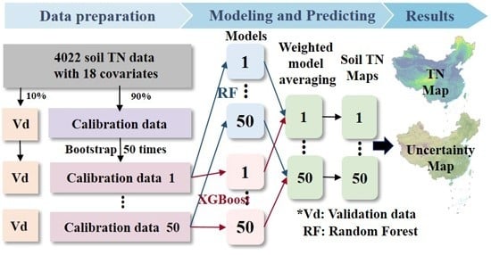
2.3. Model Development

Two machine-learning approaches named extreme gradient boosting (XGBoost) and random forest (RF) were used to produce the predictions and their lower and upper 90%. These two predictions were then ensembled by WMA.

2.3.1. Machine-Learning Approaches

The Random Forest creates a series of randomly generated classification and regression trees based on a bagging algorithm [46]. The basic idea of RF is that each tree grows independently by randomly sampling replacements from an original training set, with the unselected samples considered as out-of-bag data for testing the accuracy of the predictions. Then m covariates (m is less than the total number of the covariates) are randomly selected to split the tree at each node in an optimal way by minimizing the variance of the split groups. Each tree of the model will be at its maximum growth with no pruning, and the final prediction is the average of all fitted trees.

XGBoost is based on a gradient-boosting algorithm [47]. This method attaches importance to incorrect predictions done by prior learners and converts a series of weak and inaccurate learners to a strong predictor by weighted summation. In XGBoost, the objective function that needs to be minimized is equal to the sum of two parts, the training loss and regularization loss. Regularization is a function defined by the complexity of a tree that can avoid overfitting; shrinkage and column subsampling also play the same role.

2.3.2. Weighted Model Averaging

Each machine learning algorithm has its strengths and weaknesses [25]. Weighted model averaging is an approach combining the outcomes across different contributor models by the weighted summation. The principle of model averaging suggests the new prediction value is at least as good as any of the individual prediction value [25]. The new prediction value of ${\hat{y}}_{WMA}$ is calculated as:

$${\hat{y}}_{WMA}={\displaystyle \sum _{m=1}^M{w}_m{\hat{y}}_m}$$

(3)

where M is the number of predictors, ${\hat{y}}_{mi}$ is the prediction from the predictor m, and $w_m$ is the weight attributed to that model.

In this study, M = 2, the value of ${\hat{y}}_{WMA}$ is the weighted summation of the predictions from RF and XGBoost: ${\hat{y}}_{RF}$ and ${\hat{y}}_{XGBoost}$. The least absolute shrinkage and selection operator (LASSO) regression was used to solve for the parameters: $w_{RF}$ and $w_{XGBoost}$. The LASSO algorithm is better than the unpenalized least squares algorithms as it can enforce regularity rather than simply lead to putting all weight on the most complicated predictor, which had been proved by Hansen [18].

2.3.3. Model Calibration and Validation

After partitioning the soil samples into calibration data (90%, 3620) and validation data (10%, 402), we constructed prediction models using calibration data and their corresponding 18 covariates, and then the model performance was evaluated with 402 validation data.

For validation purposes, three indices including the determination coefficient (R²), the root mean squared error (RMSE) and the mean error (ME) were selected to estimate the prediction accuracy by the aforementioned models. Their formulae are listed as follows.

$$R^2=1-\frac{{\displaystyle \sum _{i=1}^n{(y_i-f_i)}^2}}{{\displaystyle \sum _{i=1}^n{(y_i-\overline{y})}^2}}$$

(4)

$$RMSE=\sqrt{\frac{{\displaystyle {\sum }_{i=1}^n{(y_i-f_i)}^2}}{n}}$$

(5)

$$ME=\frac{{\displaystyle {\sum }_{i=1}^n(f_i-y_i)}}{n}$$

(6)

where $\overline{y}$ is the mean of the measured data (equal-area spline interpolated values in our case), and y_i and f_i are measured and predicted values for sample i (i = 1, 2, …, n) respectively.

2.4. Uncertainty Assessment

To measure and quantify the uncertainty associated with the predictions, we generated 50 calibration datasets based on 50 times non-parametric bootstrapping. We constructed 50 RF models and 50 XGBoost models based on the 50 calibration datasets in R software with Caret (Classification and Regression Training) package [48,49]. Then the WMA assigned weight parameters to the RF and XGBoost model of each iteration using the LASSO algorithm, with the TN measurement values as the dependent variable and the TN prediction values from RF and XGBoost as independent variables. The 50 WMA models were constructed with glmnet package [50].

After applying these models on each pixel (90 × 90 m), we derived 50 maps of soil TN for each single machine learning method. We calculated the weighted summation of two maps (i.e. a RF map and a XGBoost map) obtained from one iteration and then generated 50 WMA maps. We took the average of the 50 soil TN maps as one final map of China. For clarity, the process of spatial modeling was presented in Figure S2.

For each grid point, we calculated the 90% confidence intervals (CIs) of the prediction values from each algorithm, which indicated that the true value of the TN content has 90% possibility within the interval between upper and lower CI limits. The 90% CIs is calculated in Equation (7):

$$CIs=\overline{P}\pm 1.645\frac{s}{\sqrt{n}}$$

(7)

where $\overline{P}$ is the average soil TN content of the n times predictions, and in this study, n = 50. s is the standard deviation of n times predictions.

Finally, we can calculate the uncertainty of our estimates in Equation (8):

$$U=\frac{C{I}_{upper}-C{I}_{lower}}{\overline{P}}$$

(8)

where $C{I}_{upper}$ and $C{I}_{lower}$ are the lower and upper bounds of CIs.

2.5. One-Way Analysis of Variance (ANOVA) Test

One-way ANOVA (analysis of variance) test was used to test if the value of R² differs significantly between XGBoost, RF, and WMA models.

3. Results

3.1. Importance of Covariates

The results of the average relative importance of the covariates through 50 iterations of XGBoost and RF are shown in Figure 3. The climate variables played a vital role among 18 covariates. Precipitation had relative values of about 28%, followed by land surface temperature (26%), radiation (22%), temperature (22%) and ET (21%). While elevation (24%) was the foremost topographic variable. The NDVI (26%) and NPP (22%) were of almost equal importance. The vegetation and land-use types were much less important than the other factors, with relative values of less than 12%. The importance of soil types is 23%. The prediction models assigned the highest importance to precipitation, land surface temperature and NDVI that these factors were pivotal to shape the spatial distribution pattern of soil TN.

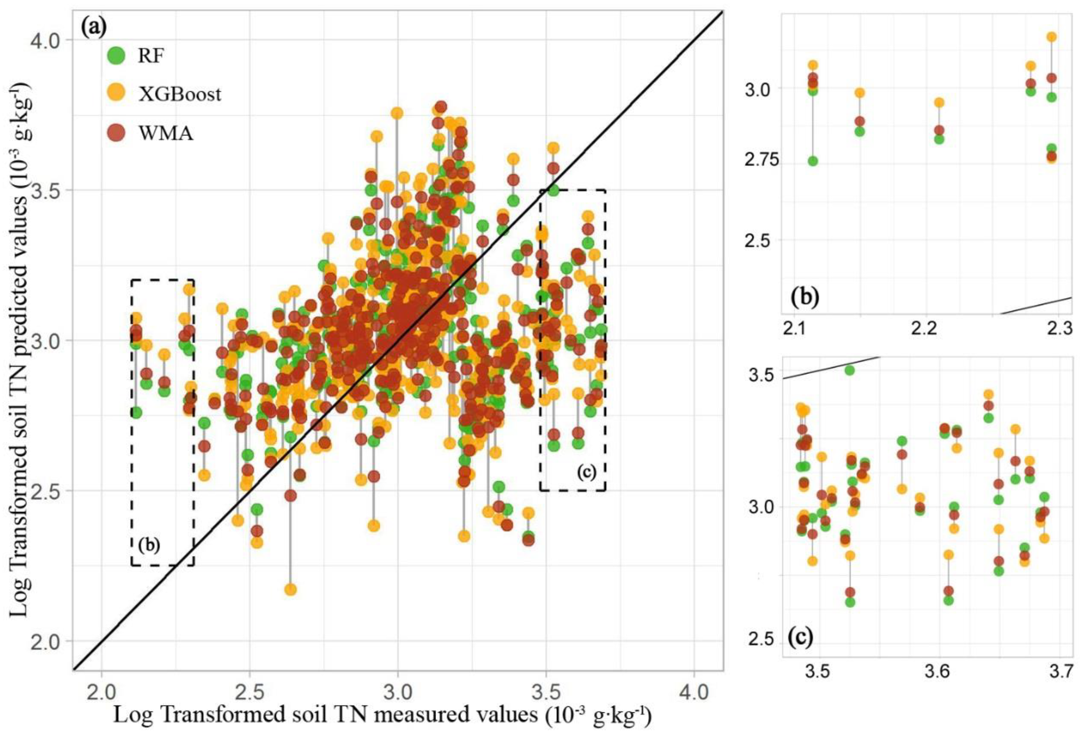
3.2. Evaluation of the Approaches

The weight parameters assigned to RF and XGBoost models through 50 iterations are summarized in Figure S3.

Table 2. Model diagnostics for independent validation.

	R2	RMSE 1 (g·kg−1)	ME 2 (g·kg−1)
XGBoost	0.34	1.20	−0.26
RF	0.38	1.18	−0.27
WMA	0.41	1.15	−0.29

¹ The root mean squared error. ² The mean error.

showed the average values of validation indices through 50 iterations of XGBoost, RF, and WMA algorithms are presented in Table 2. A plot between the measured and predicted log-transformed TN values from the three models is presented in Figure 4. Table S1 showed the output of the ANOVA analysis and whether there is a significant difference between the three models’ average R².

The ME values in the three models were very small, which indicated that the predictions were roughly unbiased. The R² of the Random Forest was always 0.04 higher, and the RMSE was 0.02 g·kg⁻¹ lower than those for the XGBoost method. Therefore, the RF models were always preferred and assinged bigger weight parameters than XGBoost in constructing a WMA model (Figure S3). Figure 4a showed that both RF and XGBoost overestimated predictions in low values of targets and underestimated high values. Compared with each other, RF and XGBoost produced better predictions for the data points with low (Figure 4b) and high (Figure 4c) TN contents, respectively. After the two models were weight-averaged, consequently, the model performance was best with R² of 0.41 and RMSE value of 1.15 g·kg⁻¹; this showed that the WMA could explain 41% of the spatial variation in the TN contents. The results of one-way ANOVA showed (p = 0.000) that there was a statistically significant difference in the mean R² values between WMA, RF and XGBoost.

The three uncertainty results for each validation data with the 50 XGBoost, 50 RF, and 50 WMA models are shown in Figure 5. The mean uncertainty value of WMA is 0.05, much smaller than that of XGBoost (0.14) and RF (0.08). For each validation data, the finest result always derived from the WMA method, except for the two points emphasized with orange color in Figure 5, which demonstrated that there was a high probability that the prediction uncertainty could be reduced by using the WMA approach.

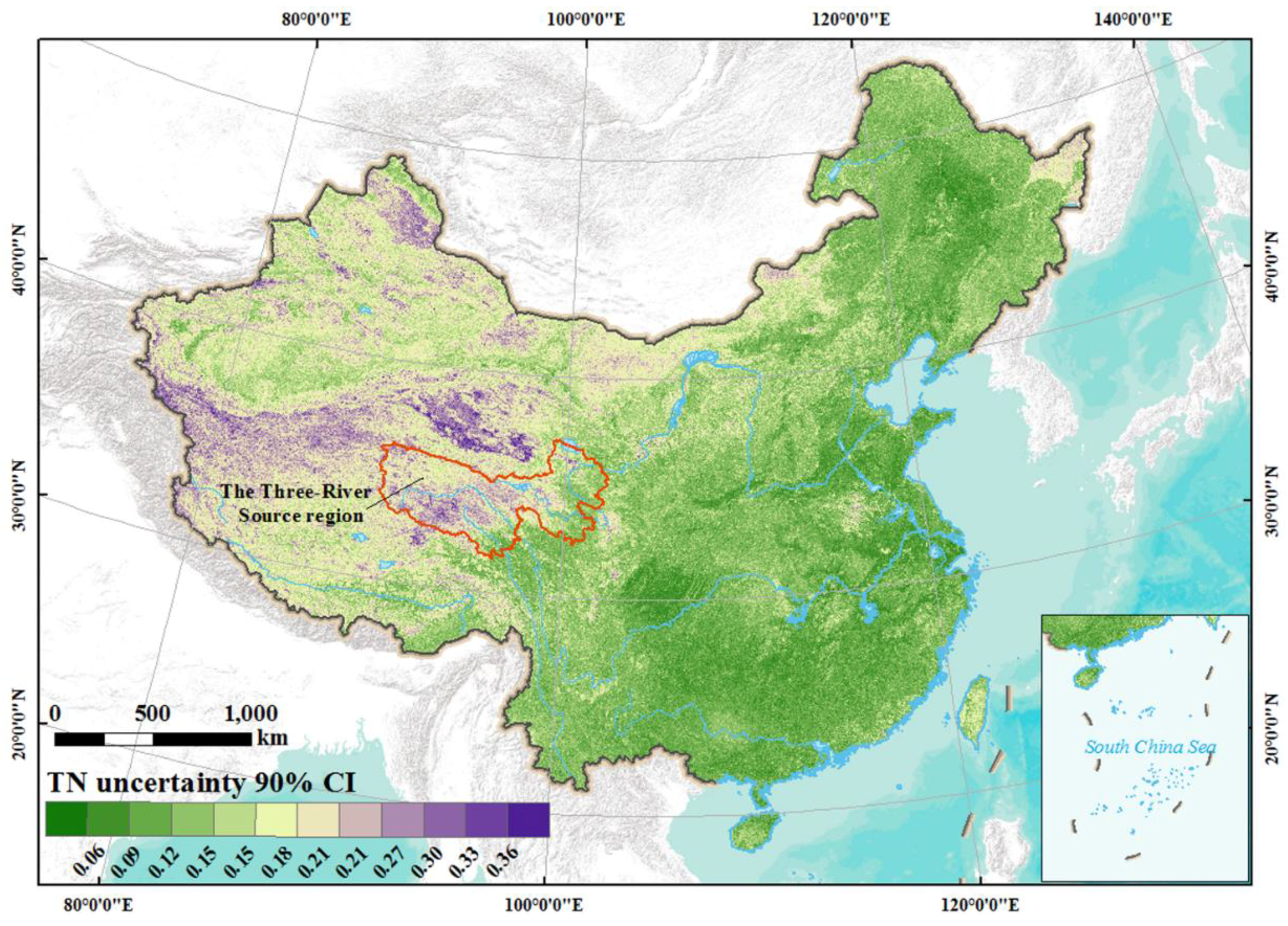
3.3. Mapping of Soil TN and Its Uncertainty

A national scale map of soil TN was constructed by WMA at 90 m resolution (Figure 6), and its increased details also were displayed at a gradually finer scale. This map clearly shows the total geographical distribution of soil TN. The TN content in the topsoil (0–20 cm) ranged from 0.13 to 9.92 g·kg⁻¹ and averaged 1.648 g·kg⁻¹ across China. The TN contents varied considerably and were distributed unevenly. The TN contents were high (>4.8 g·kg⁻¹) in eastern areas of the Tibetan Plateau, the central Qilian Mountains, and the northern section of the Greater Khingan Range, and were low (<0.8 g·kg⁻¹) between 35°N and 42.5°N, in the Tarim Basin, Qaidam Basin and western Inner Mongolia Plateau, particularly in the desert areas. The TN contents were also low on the Loess Plateau and the North China Plain.

We mapped the spatial distribution of the uncertainty based on the 50 WMA soil TN map (Figure 7). The uncertainty values were low in the southeastern area where there were many soil profiles. Equally, the uncertainty values were high in the western area because of the low density of the soil samples. The large tracts of desert land and high-attitude depopulated zone make it difficult to sample by soil surveyors, which thus lead to the large uncertainty in these regions when using DSM technology. It is also noteworthy that the uncertainty was greatest in the Kunlun Mountains, Altun Mountains and the Three-River Source region, the source of the Yangtze, the Yellow and the Lantsang Rivers. These areas have a complex and highly fragmented landscape structure which can hardly be detected by the sparse soil data used in this study.

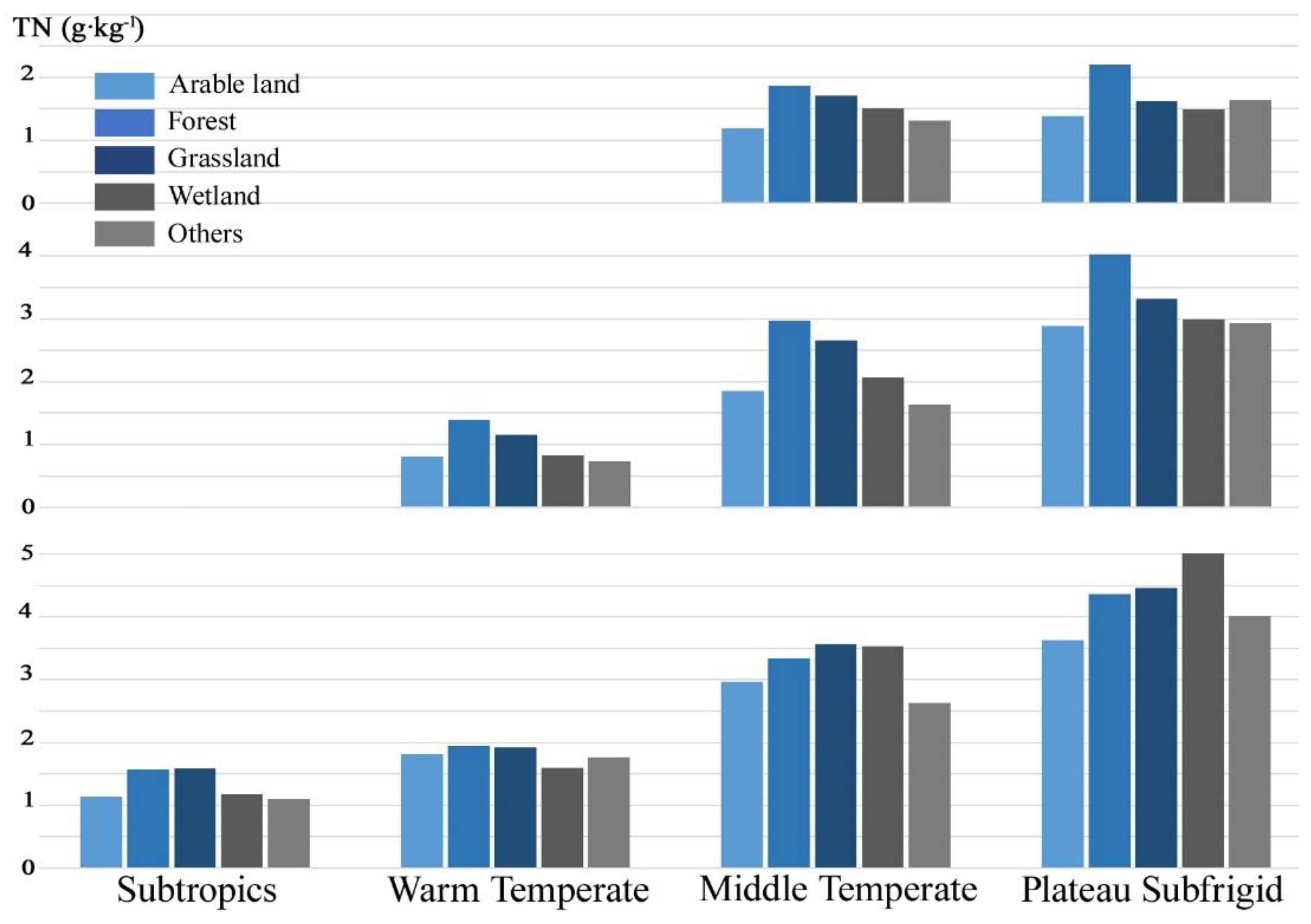
3.4. Soil TN of Different Soil Types and Land-Use Types

Soil TN contents at a depth of 0–20 cm under different soil types and land-use patterns are shown in Table S2 and Figure 8. The soil TN varied considerably across the soil groups and ranked in the following order: Histosols > Phaeozems > Chernozems > Luvisols > Cryosols > Kastanozems > Acrisols > Anthrosols > Cambisols > Calcisols > Solonchaks > Arenosols > Fluvisols. The TN content also showed dramatic differences between land-use types. At the great group level, TN contents were highest in the forest, followed by grassland, cropland and construction land, while lowest in unused land. In terms of the subgroups, there was a direct relationship between high coverage and high soil TN content in the group of forest and grassland. Wetland held the highest TN content among the unused land.

The average TN contents for the different land-use types in each climate zone are listed in Figure 9. The TN contents increased as precipitation increased and temperature decreased. In each climatic zone, the TN contents in arable land were noticeably lower than that of forest and grassland. The drier the climate was, the greater were the differences in soil TN contents between arable land and the other two vegetated land-use types. In arid regions, the soil TN contents in arable land are only about half of that in the forest.

We converted TN contents of arable land into six grades (

Table 3. Soil TN grades, with corresponding areas (10¹⁰ km²) and proportion.

Grade		1	2	3	4	5	6
TN content (g·kg−1)		>2	1.5–2	1.0–1.5	0.75–1	0.5–0.75	<0.5
Arable land	area	1.57	2.09	4.43	3.39	2.09	0.17
	proportion	11.4%	15.2%	32.3%	24.7%	15.2%	1.2%

) according to the rules of the National Soil Survey Office [51]. The TN contents were most in Grade 3 (32.3%) which between 1.0 and 1.5 g·kg⁻¹. Nitrogen-lacking soil with TN less than 1.0 g·kg⁻¹ accounted for 41.3%.

4. Discussion

4.1. Quality of the Prediction

In general, the prediction ability of RF was better than XGBoost in 50 iterations of bootstrapping. RF model can reduce over-learning and over-fitting [46], it was often the best one among multiple machine learning methods, which have been confirmed by many studies [22,52]. However, RF model inherited the insensitivity to outliers from recursive partitioning and tree averaging, while XGBoost trained subsequent models using residuals and was more sensitive to outliers [46,47]. Among the soil data used in this study, some points with extremely high TN contents were considered outliers in statistics. We confirmed the authenticity of these data and kept the records. For these high values, XGBoost model had better prediction accuracy, as shown in Figure 4. Therefore, WMA ensembled two models, kept the advantages and discarded the inaccurate aspect of each algorithm [25]. Consequently, WMA exhibited the best competence for capturing the spatial variation of soil TN and reducing prediction uncertainty as well. The results from many other studies have been similar, with researchers concluding that the results were better from an ensemble of different DSM models than from a single model [22,23]. Hence, we suggest that it is often useful to combine the predictions of several models because the large variance can be balanced through averaging.

We compared our data with those from other published studies and found that our combined model performed better than other models applied at the national scale for China. Shangguan et al. [53] developed a 30 arc-second (1 km) resolution soil TN map with the polygon linkage method. Li et al. [54] produced a map of TN in topsoil by combining a multiple regression model and neural networks. The mean relative error for the predicted value was 61.06%, which was higher than that in our study (49.17%). Our models were suitable for producing a 90-m resolution national map of soil TN that was more reliable, provided detailed information about the spatial variation in TN, and followed the specifications of the GlobalSoilMap [55].

4.2. Spatial Distribution of Soil TN

The distribution map (Figure 5) revealed the spatial pattern of soil TN and gave us insights into how the environment influenced the TN in soil. As one of soil formation factors, topography plays an important role in TN modeling and can determine the hydrothermal conditions and distribution of soil-forming substances [10]. Soil TN increased significantly as the elevation increased, possibly reflecting less human disturbance and better moisture-temperature conditions at high altitude [17,28,29]. Precipitation and temperature acted as climate proxies and the most robust predictors of TN in our study as shown in Figure 3 and Figure 9. They affected the spatial distribution of TN via changes in the soil moisture content and soil temperature [56]. The activity and species of the bacteria that decompose and convert organic matter is limited in low temperature [19,57]. The NDVI and NPP are also good predictors of the soil TN as shown in Figure 3 and Figure 8, as the vegetation productivity and biomass are correlated with the amount of litter that is returned to the soil [20]. Generally, the TN contents increased with increases in elevation, precipitation and vegetation cover density, decreases in temperature. Soil TN gradually accumulated and eventually reached high levels via slow decomposition, accumulation of biomass, and weak leaching. Thus, we could expect the geographic trend shown in Figure 6, with higher soil TN in Cryosols in the alpine meadow area of the eastern Tibet plateau, and in Phaeozems, Chernozems and Luvisols in the northern forest zone of the Greater Khingan Range, while the lower TN mainly in the desert area. These distribution patterns are consistent with those presented on the national TN maps produced by Li et al. [54] and Shangguan et al. [53].

4.3. Uncertainty in Soil TN Prediction

The amount of importance in assessing the uncertainty is almost as great as that in making a prediction map [58], uncertainty map helped researchers to identify the source of the uncertainty and propose solutions [59,60]. To obtain a very reliable prediction, we can control the uncertainty of soil TN map from two aspects.

First, we can deal with the uncertainty introduced by a limited number of covariates by adding more variables that are either more relevant or more precise into the model’s dataset. In this study, the elevation drops dramatically in the mountainous areas; in these places, the uncertainty is large, reflecting the high heterogeneity in the adjacent geographical factors, which is further translated into inaccurate descriptions of variables when mapped at coarse resolutions. When downscaling, these uncertainties will be further propagated to the soil TN predictions. Moreover, the drainage area of the Three-River Source region is 237,957 km², or 65.9% of the total area [61]. The soils here are susceptible to erosion by runoff [62], so considerable amounts of soil TN are probably redistributed [63], thereby weakening the relationship between soil TN and covariates. It would therefore be useful to add quantitative estimates of either soil erosion or the soil loss potential to improve the accuracy of the TN estimates [64].

Second, where the uncertainty originates from insufficient soil profiles, the density of the sampling network could be increased and more samples could be collected. With an adequate dataset, we can capture spatial variance explained by environmental covariates more precisely. When establishing a new database, areas with low certainty should be emphasized and should be a priority for further database investment [65,66].

4.4. Effect of Land Use on Soil TN Contents

Figure 8 and Figure 9 demonstrated that lower TN contents in cultivated soils than in soils under natural vegetation cover, similar results were recorded by previous studies [20,67]. Human activities play a dominant role in controlling the TN contents in a specific climate region [11]. Tillage and other agricultural strategies will destroy the physical protective layer and promote soil respiration, thus accelerate the decomposition of organic matter [68,69]. Zhao et al. [70] have certified that after 50 years of cultivation, the TN contents in 0–20 cm decreased by 67%–68%. Consequently, soil TN dropped dramatically when land use shifted from forest or grassland to arable land [67,71,72,73].

The soil TN levels were low across large-scale cultivated areas, as shown in Table 3, which would have a serious constraint on agricultural yields. Many farmers chose to expand acreage to reach a high total value of crop production, thus China’s landscape has undergone large changes since the 1980s, with great losses of woodland and grassland and corresponding gains in cropland [74]. Blind reclamation resulted in soil nutrient loss, soil erosion, environmental deterioration and a vicious circle of poverty. A turnaround appeared from 1999 onwards with a rebound in forest and grassland, when the Returning Farmland to Forest Program (RFFP) was introduced. The RFFP compensated farmers for giving marginal cropland back to forest or grassland in order to increase forest cover, improve soil quality and alleviate poverty [75]. Soil TN concentration increased after the establishment of the woodland or grassland on abandoned cropland [70,76]. However, compared with rapid soil degradation caused by injudicious land use and management, the recovery of soil fertility would take a long period of time once the fragile environment was destroyed [70]. Incontrovertibly, there is an important need to make policy decisions about land-use planning that take account of the local conditions rather than applying experience mechanically. These N-rich soils should be used for activities that are suitable for their soil formation characteristics and environmental histories such as forestry and animal husbandry, and these N-lacking soils in arable land can be improved by applying N fertilizer rationally and returning straw [77].

4.5. Limitations and Perspectives

In 1980, the annual consumption of nitrogen fertilizer in China had exceeded 9 million tons, and it increased dramatically to over 22 million tons in 2017 [78]. The environmental cost of immoderate nitrogen fertilizer has become a dilemma that causes environmental degradation in China including soil acidification, air pollution, water pollution and ecosystem diversity decline [71,79,80]. Soil TN content should be monitored so as to know how this has changed since the 1980s under human activities, especially for the nitrogen application. The accuracy of our TN map is limited by the size of the soil database which cannot completely capture the large variation in such a large country. Another limitation of map accuracy results from the relatively low quality of environmental covariates corresponding to the soil sampling year. However, the modeling and predicting procedure proposed in this study can be easily transferred to other time periods under GlobalSoilMap specifications and further applied to the monitoring of soil TN dynamics.

Several issues should be carefully addressed in subsequent works. First, the uncertainties from inaccuracy environmental covariates and inadequate soil profiles should be handled by integrating higher-quality data sources and supplementing samples as mentioned in Section 4.3. Second, some soil properties which correlate with soil TN (e.g., soil texture, pH, soil organic carbon) should be incorporated as environmental covariates to further improve map accuracy. Third, it is worth considering total nitrogen simulation in three dimensions.

Nevertheless, all of the data for mapping soil TN in this study are the most detailed dataset we can acquire for China. Our soil TN map can fill the gap in national TN inventorying at a high spatial resolution and thereby function as a baseline to monitor how the TN content and spatial distribution change with human-induced changes in land use, the development of industry and agriculture, population growth, land management, and climate change. Furthermore, governmental departments that make decisions can formulate corresponding management strategies to improve nitrogen sequestration and mitigate global warming, based on the soil-monitoring network.

5. Conclusions

Our study is the first contribution of mapping Chinese soil total nitrogen at 90 m resolution. We constructed the prediction model by combining a random forest model with an extreme gradient boosting model. The conclusions of this study are listed below:

• Using the weighted average of these two models, a reasonable result was obtained, with the lowest RMSE (1.15 g·kg⁻¹) and the highest R² (0.41) compared with individual models, that explained 41% of the spatial discrepancy in the soil TN contents and reduced the prediction uncertainty as well.
• The TN map showed high spatial heterogeneity, with the spatial variation influenced by variables related to climate, relief and organisms. The spatial trends were similar to previous TN maps in coarser resolution, with high TN in the eastern Tibetan Plateau and north-eastern China, and low TN in the desert area.
• The uncertainty map can help policymakers and stakeholders to understand the reliability of the map produced in our study. It should be noted that the uncertainties can be reduced by using more covariates or supplementing the number of soil profiles in the future.

As the most quantitative and precise estimate of the soil TN contents at the national scale, our TN map can serve as a baseline to monitor soil TN dynamics, formulate land-use strategies and support biogeochemical simulations.

References

1. Sinfield, J.V.; Fagerman, D.; Colic, O. Evaluation of sensing technologies for on-the-go detection of macro-nutrients in cultivated soils. Comput. Electron. Agric. 2010, 70, 1–18. [Google Scholar] [CrossRef]
2. Reeves, M.; Lal, R.; Logan, T.; Sigarán, J. Soil Nitrogen and Carbon Response to Maize Cropping System, Nitrogen Source, and Tillage. Soil Sci. Soc. Am. J. 1997, 61, 1387–1392. [Google Scholar] [CrossRef]
3. Vitousek, P.M.; Porder, S.; Houlton, B.Z.; Chadwick, O.A. Terrestrial phosphorus limitation: Mechanisms, implications, and nitrogen–phosphorus interactions. Ecol. Appl. 2010, 20, 5–15. [Google Scholar] [CrossRef] [PubMed] [Green Version]
4. Ledley, T.S.; Sundquist, E.T.; Schwartz, S.E.; Hall, D.K.; Fellows, J.D.; Killeen, T.L. Climate change and greenhouse gases. EOS Trans. Am. Geophys. 2013, 80, 453–458. [Google Scholar] [CrossRef] [Green Version]
5. Li, C.S. Quantifying greenhouse gas emissions from soils: Scientific basis and modeling approach. Soil Sci. Plant Nutr. 2007, 53, 344–352. [Google Scholar] [CrossRef] [Green Version]
6. Carpenter, S.R.; Caraco, N.F.; Corell, D.L.; Howarth, R.W.; Sharpley, A.N.; Smith, V.H. Nonpoint pollution of surface waters with phosphorus and nitrogen. Ecol. Appl. 1998, 8, 559–568. [Google Scholar] [CrossRef]
7. Batjes, N.H. Total carbon and nitrogen in the soils of the world. Eur. J. Soil Sci. 1996, 47, 151–163. [Google Scholar] [CrossRef]
8. Arrouays, D.; Deslais, W.; Badeau, V. The carbon content of topsoil and its geographical distribution in France. Soil Use Manag. 2001, 17, 7–11. [Google Scholar] [CrossRef]
9. McBratney, A.B.; Santos, M.L.M.; Minasny, B. On digital soil mapping. Geoderma 2003, 117, 3–52. [Google Scholar] [CrossRef]
10. Jenny, H. Factors of Soil Formation; McGraw-Hill: New York, NY, USA, 1941. [Google Scholar]
11. Wang, S.; Wang, X.; Ouyang, Z. Effects of land use, climate, topography and soil properties on regional soil organic carbon and total nitrogen in the Upstream Watershed of Miyun Reservoir, North China. J. Environ. Sci. 2012, 24, 387–395. [Google Scholar] [CrossRef]
12. Qiao, J.; Zhu, Y.; Jia, X.; Huang, L.; Shao, M. Vertical distribution of soil total nitrogen and soil total phosphorus in the critical zone on the loess plateau, China. Catena 2018, 166, 310–316. [Google Scholar] [CrossRef]
13. Selige, T.; Böhner, J.; Schmidhalter, U. High resolution topsoil mapping using hyperspectral image and field data in multivariate regression modeling procedures. Geoderma 2006, 136, 235–244. [Google Scholar] [CrossRef]
14. Wang, K.; Zhang, C.; Li, W. Predictive mapping of soil total nitrogen at a regional scale: A comparison between geographically weighted regression and cokriging. Appl. Geogr. 2013, 42, 73–85. [Google Scholar] [CrossRef]
15. Elbasiouny, H.; Abowaly, M.; Abu_Alkheir, A.; Gad, A. Spatial variation of soil carbon and nitrogen pools by using ordinary Kriging method in an area of north Nile Delta, Egypt. Catena 2014, 113, 70–78. [Google Scholar] [CrossRef]
16. Kou, D.; Ding, J.Z.; Li, F.; Wei, N.; Fang, K.; Yang, G.; Zhang, B.; Liu, L.; Qin, S.; Chen, Y.; et al. Spatially-explicit estimate of soil nitrogen stock and its implication for land model across Tibetan alpine permafrost region. Sci. Total Environ. 2019, 650, 1795–1804. [Google Scholar] [CrossRef]
17. Shahbazi, F.; Hughes, P.; McBratney, A.B.; Minasny, B.; Malone, B.P. Evaluating the spatial and vertical distribution of agriculturally important nutrients—Nitrogen, phosphorous and boron—In North West Iran. Catena 2019, 173, 71–82. [Google Scholar] [CrossRef]
18. Hansen, B.E. ECONOMETRICS; Department of Economics, University of Wisconsin: Madison, WI, USA, 2019; p. 846. Available online: http://www.ssc.wisc.edu/~bhansen/econometrics/ (accessed on 19 August 2019).
19. Wang, S.; Zhuang, Q.L.; Wang, Q.B.; Jin, X.; Han, C. Mapping stocks of soil organic carbon and soil total nitrogen in Liaoning Province of China. Geoderma 2017, 305, 250–263. [Google Scholar] [CrossRef]
20. Wang, S.; Jin, X.; Adhikari, K.; Li, W.; Yu, M.; Bian, Z.; Wang, Q. Mapping total soil nitrogen from a site in northeastern China. Catena 2018, 166, 134–146. [Google Scholar] [CrossRef]
21. Zhou, Y.; Webster, R.; Viscarra Rossel, R.A.; Shi, Z.; Chen, S. Baseline map of soil organic carbon in Tibet and its uncertainty in the 1980s. Geoderma 2019, 334, 124–133. [Google Scholar] [CrossRef]
22. Nussbaum, M.; Spiess, K.; Baltensweiler, A.; Grob, U.; Keller, A.; Greiner, L.; Schaepan, M.E.; Papritz, A. Evaluation of digital soil mapping approaches with large sets of environmental covariates. Soil 2018, 4, 1–22. [Google Scholar] [CrossRef] [Green Version]
23. Chen, S.C.; Liang, Z.Z.; Webster, R.; Zhang, G.L.; Zhou, Y.; Teng, H.F.; Hu, B.F.; Arrouays, D.; Shi, Z. A high-resolution map of soil pH in China made by hybrid modeling of sparse soil data and environmental covariates and its implications for pollution. Sci. Total Environ. 2019, 655, 273–283. [Google Scholar] [CrossRef] [PubMed]
24. Boehmke, B.C.; Greenwell, B.M. Hands-On Machine Learning with R, 1st ed.; CRC Press: Boca Raton, FL, USA, 2019; in press; Available online: https://bradleyboehmke.github.io/HOML/ (accessed on 6 December 2019).
25. Malone, B.P.; Minasny, B.; Odgers, N.P.; McBrantney, A. Using model averaging to combine soil property rasters from legacy soil maps and from point data. Geoderma 2014, 232–234, 34–44. [Google Scholar] [CrossRef]
26. Xu, Y.; Smith, S.E.; Grunwaldb, S.; Abd-Elrahman, A.; Wani, S.P.; Nair, V.D. Estimating soil total nitrogen in smallholder farm settings using remote sensing spectral indices and regression kriging. Catena 2017, 163, 111–122. [Google Scholar] [CrossRef] [Green Version]
27. Xu, G.; Cheng, S.; Li, P.; Li, Z.; Gao, H.; Yu, K.; Lu, K.; Shi, P.; Cheng, Y.; Zhao, B. Soil total nitrogen sources on dammed farmland under the condition of ecological construction in a small watershed on the Loess Plateau, China. Ecol. Eng. 2018, 121, 19–25. [Google Scholar] [CrossRef]
28. Zhao, Z.; Zhang, X.; Dong, S.; Wu, Y.; Liu, S.; Su, X.; Wang, X.; Zhang, Y.; Tang, L. Soil organic carbon and total nitrogen stocks in alpine ecosystems of Altun Mountain National Nature Reserve in dry China. Environ. Monit. Assess. 2018, 191, 40. [Google Scholar] [CrossRef] [PubMed]
29. Liu, H.; Cao, L.; Zeng, J. Spatial distribution of soil nitrogen in gully hillsides of Sejila Mountain, Southeastern Tibet. Acta Ecol. Sin. 2016, 36, 127–133. [Google Scholar]
30. National Soil Survey Office. Chinese Soil Genus Records; China Agriculture Press: Beijing, China, 1993; Volume 1, (In Chinese).
31. National Soil Survey Office. Chinese Soil Genus Records; China Agriculture Press: Beijing, China, 1994; Volume 2, (In Chinese).
32. National Soil Survey Office. Chinese Soil Genus Records; China Agriculture Press: Beijing, China, 1994; Volume 3, (In Chinese).
33. National Soil Survey Office. Chinese Soil Genus Records; China Agriculture Press: Beijing, China, 1995; Volume 4, (In Chinese).
34. National Soil Survey Office. Chinese Soil Genus Records; China Agriculture Press: Beijing, China, 1995; Volume 5, (In Chinese).
35. National Soil Survey Office. Chinese Soil Genus Records; China Agriculture Press: Beijing, China, 1996; Volume 6, (In Chinese).
36. Gregorich, E.G.; Carter, M.R.; Angers, D.A.; Monreal, C.M.; Ellert, B.H. Towards a minimum data set to assess soil organic-matter quality in agricultural soils. Can. J. Soil Sci. 1994, 74, 367–385. [Google Scholar] [CrossRef] [Green Version]
37. Bishop, T.F.A.; McBratney, A.B.; Laslett, G.M. Modeling soil attribute depth functions with equal-area quadratic smoothing splines. Geoderma 1999, 91, 27–45. [Google Scholar] [CrossRef]
38. Malone, B.P.; Mcbratney, A.B.; Minasny, B.; Laslett, G.M. Mapping continuous depth functions of soil carbon storage and available water capacity. Geoderma 2009, 154, 138–152. [Google Scholar] [CrossRef]
39. Conrad, O.; Bechtel, B.; Bock, M.; Dietrich, H.; Fischer, E.; Gerlitz, L.; Wehberg, J.; Wichmann, V.; Böhner, J. System for Automated Geoscientific Analyses (SAGA) v. 2.1.4. Geosci. Model. Dev. 2015, 8, 1991–2007. [Google Scholar] [CrossRef] [Green Version]
40. Tucker, C.J.; Pinzon, J.E.; Brown, M.E. Global Inventory Modeling and Mapping Studies; NA94apr15b.n11-VIg, 2.0; Global Land Cover Facility, University of Maryland: College Park, MD, USA, 2004. [Google Scholar]
41. Prince, S.D.; Small, J. AVHRR Global Production Efficiency Model, 1981–2000; The Global Land Cover Facility, University of Maryland: College Park, MD, USA, 2003. [Google Scholar]
42. Goovaerts, P. Using elevation to aid the geostatistical mapping of rainfall erosivity. Catena 1999, 34, 227–242. [Google Scholar] [CrossRef]
43. Shi, X.Z.; Yu, D.S.; Warner, E.D.; Pan, X.Z.; Petersen, G.W.; Gong, Z.G.; Weindorf, D.C. Soil database of 1: 1,000,000 digital soil survey and reference system of the chinese genetic soil classification system. Soil Horiz. 2004, 45, 129–136. [Google Scholar] [CrossRef]
44. IUSS Working Group WRB. World Reference Base for Soil Resources 2014, Update 2015 International Soil Classification System for Naming Soils and Creating Legends for Soil Maps; Food and Agriculture Organization of the United Nations: Rome, Italy, 2015. [Google Scholar]
45. Shi, X.Z.; Yu, D.S.; Xu, S.X.; Warner, E.D.; Wang, H.J.; Sun, W.X.; Zhao, Y.C.; Gong, Z.T. Cross-reference for relating Genetic Soil Classification of China with WRB at different scales. Geoderma 2010, 155, 344–350. [Google Scholar] [CrossRef]
46. Breiman, L. Random forests. Mach. Learn. 2001, 45, 5–32. [Google Scholar] [CrossRef] [Green Version]
47. Friedman, J.H. Greedy function approximation: A gradient boosting machine. Ann. Stat. 2001, 29, 1189–1232. [Google Scholar] [CrossRef]
48. R Core Team. R: A Language and Environment for Statistical Computing; R Foundation for Statistical Computing: Vienna, Austria, 2013. [Google Scholar]
49. Kuhn, M. Caret: Classification and Regression Training. R Package Version 6.0-84. 2019. Available online: https://CRAN.R-project.org/package=caret (accessed on 27 April 2019).
50. Friedman, J. Glmnet: Lasso and Elastic-Net Regularized Generalized Linear Models. R Package Version 3.0-2. 2019. Available online: https://cran.r-project.org/web/packages/glmnet/index.html (accessed on 11 December 2019).
51. National Soil Survey Office. Chinese Soil; China Agriculture Press: Beijing, China, 1998; (In Chinese).
52. Fernandez-Delgado, M.; Cernadas, E.; Barro, S.; Amorim, D. Do we need hundreds of classifiers to solve real world classification problems? J. Mach. Learn. Res. 2014, 15, 3133–3181. [Google Scholar]
53. Shangguan, W.; Dai, Y.; Liu, B.; Zhu, A.X.; Duan, Q.Y.; Wu, L.Z.; Ji, D.Y.; Ye, A.Z.; Yuan, H.; Zhang, Q.; et al. A China data set of soil properties for land surface modeling. J. Adv. Model. Earth Syst. 2013, 5, 212–224. [Google Scholar] [CrossRef]
54. Li, Q.Q.; Yue, T.X.; Fan, Z.M.; Du, Z.P.; Chen, C.F.; Lu, Y.M. Spatial simulation of topsoil TN at the national scale in China. Geogr. Res. 2010, 29, 1981–1992. (In Chinese) [Google Scholar]
55. Arrouays, D.; Grundy, M.G.; Hartemink, A.E.; Hempel, J.W.; Heuvelink, G.B.M.; Hong, S.Y.; Lagacherie, P.; Lelyk, G.; McBratney, A.B.; McKenzie, N.J.; et al. Globalsoilmap: Toward a fine-resolution global grid of soil properties. Adv. Agron. 2014, 125, 93–134. [Google Scholar]
56. Follett, R.F.; Stewart, C.E.; Pruessner, E.G.; Kimble, J.M. Effects of climate change on soil carbon and nitrogen storage in the US Great Plains. J. Soil Water Conserv. 2012, 67, 331–342. [Google Scholar] [CrossRef] [Green Version]
57. Tsui, C.C.; Chen, Z.S.; Hsieh, C.F. Relationships between soil properties and slope position in a lowland rain forest of southern Taiwan. Geoderma 2004, 123, 131–142. [Google Scholar] [CrossRef]
58. Macmillan, R.A.; Moon, D.E.; Coupé, R.A.; Phillips, N. Predictive Ecosystem Mapping (PEM) for 8.2 Million ha of Forestland. In Digital Soil Mapping: Bridging Research, Environmental Application, and Operation; Boettinger, J.L., Howell, D.W., Moore, A.C., Hartemink, A.E., Kienast-Brown, S., Eds.; Springer: Dordrecht, The Netherlands, 2010; Volume 2, pp. 337–356. [Google Scholar]
59. Zhou, Y.; Hartemink, A.E.; Shi, Z.; Liang, Z.Z.; Lu, Y.L. Land use and climate change effects on soil organic carbon in North and Northeast China. Sci. Total Environ. 2019, 647, 1230–1238. [Google Scholar] [CrossRef] [PubMed]
60. Liang, Z.Z.; Chen, S.C.; Yang, Y.Y.; Zhao, R.Y.; Shi, Z.; Rossel, R.A.V. National digital soil map of organic matter in topsoil and its associated uncertainty in 1980’s China. Geoderma 2019, 335, 47–56. [Google Scholar] [CrossRef]
61. Hu, M.Q.; Mao, F.; Sun, H.; Hou, Y.Y. Study of normalized difference vegetation index variation and its correlation with climate factors in the three-river-source region. Int. J. Appl. Earth Obs. Geoinf. 2011, 13, 24–33. [Google Scholar] [CrossRef]
62. Teng, H.F.; Hu, J.; Zhou, Y.; Zhou, L.Q.; Shi, Z. Modeling and mapping soil erosion potential in China. J. Integr. Agric. 2019, 18, 251–264. [Google Scholar] [CrossRef] [Green Version]
63. Peng, J.T.; Li, G.S.; Fu, W.L.; Yi, X.S.; Lan, J.C.; Yuang, B. Temporal-spatial variations of total nitrogen in the degraded grassland of Three-River Headwaters region in Qinghai Province. Environ. Sci. 2012, 33, 2490–2496. [Google Scholar]
64. Chen, S.C.; Martin, M.P.; Saby, N.P.; Walter, C.; Angers, D.A.; Arrouays, D. Fine resolution map of top-and subsoil carbon sequestration potential in France. Sci. Total Environ. 2018, 630, 389–400. [Google Scholar] [CrossRef]
65. Hewitt, A.; Barringer, J.; Forrester, G.; McNeill, S.J. Soilscapes Basis for Digital Soil Mapping in New Zealand. In Digital Soil Mapping: Bridging Research, Environmental Application, and Operation; Boettinger, J.L., Howell, D.W., Moore, A.C., Hartemink, A.E., Kienast-Brown, S., Eds.; Springer: Dordrecht, The Netherlands, 2010; Volume 2, pp. 297–307. [Google Scholar]
66. Liang, Z.Z.; Chen, S.C.; Yang, Y.Y.; Zhou, Y.; Shi, Z. High-resolution three-dimensional mapping of soil organic carbon in China: Effects of SoilGrids products on national modeling. Sci. Total Environ. 2019, 685, 480–489. [Google Scholar] [CrossRef]
67. Murty, D.; Kirschbaum, M.U.F.; Mcmurtrie, R.E.; McGilvray, A. Does conversion of forest to agricultural land change soil carbon and nitrogen? A review of the literature. Glob. Chang. Biol. 2002, 8, 105–123. [Google Scholar] [CrossRef]
68. Wang, X.J.; Gong, Z.T. Assessment and analysis of soil quality changes after eleven years of reclamation in subtropical China. Geoderma 1998, 81, 339–355. [Google Scholar] [CrossRef]
69. Wang, Y.; Wang, S.; Adhikari, K.; Wang, Q.B.; Sui, Y.Y.; Xin, G. Effect of cultivation history on soil organic carbon status of arable land in northeastern China. Geoderma 2019, 342, 55–64. [Google Scholar] [CrossRef]
70. Zhao, W.Z.; Xiao, H.L.; Liu, Z.M.; Li, J. Soil degradation and restoration as affected by land use change in the semiarid Bashang area, northern China. Catena 2005, 59, 173–186. [Google Scholar] [CrossRef]
71. Guo, L.B.; Gifford, R.M. Soil carbon stocks and land use change: A meta analysis. Glob. Chang. Biol. 2002, 8, 345–360. [Google Scholar] [CrossRef]
72. Sahani, U.; Behera, N. Impact of deforestation on soil physicochemical characteristics, microbial biomass and microbial activity of tropical soil. Land Degrad. Dev. 2001, 12, 93–105. [Google Scholar] [CrossRef]
73. Berihu, T.; Girmay, G.; Sebhatleab, M.; Berhane, E.; Zenebe, A.; Sigua, G.C. Soil carbon and nitrogen losses following deforestation in Ethiopia. Agron. Sustain. Dev. 2017, 37, 1. [Google Scholar] [CrossRef] [Green Version]
74. Hu, Y.; Zhang, X.Z.; Mao, R.; Gong, D.Y.; Liu, H.B.; Yang, J. Modeled responses of summer climate to realistic land use/cover changes from the 1980s to the 2000s over eastern China. J. Geophys. Res. Atmos. 2015, 120, 167–179. [Google Scholar] [CrossRef]
75. Zinda, J.A.; Trac, C.J.; Zhai, D.; Harrell, S. Dual-function forests in the returning farmland to forest program and the flexibility of environmental policy in china. Geoforum 2016, 78, 119–132. [Google Scholar] [CrossRef] [Green Version]
76. Song, Y.; Yao, Y.F.; Qin, X.; Wei, X.R.; Jia, X.X.; Shao, M.G. Response of carbon and nitrogen to afforestation from 0 to 5 m depth on two semiarid cropland soils with contrasting inorganic carbon concentrations. Geoderma 2020, 357, 113940. [Google Scholar] [CrossRef]
77. Jiang, Y.; Rao, L.; Sun, K.; Han, Y.; Guo, X. Spatio-temporal distribution of soil nitrogen in Poyang lake ecological economic zone (South-China). Sci. Total Environ. 2018, 626, 235–243. [Google Scholar] [CrossRef]
78. Chinese Statistic Almanac of 1999. Available online: http://www.stats.gov.cn/yearbook/indexC.htm (accessed on 20 September 1999).
79. Ju, X.T.; Xing, G.X.; Chen, X.P.; Zhang, S.L.; Zhang, L.J.; Liu, X.J.; Cui, Z.L.; Yin, B.; Christie, P.; Zhu, Z.L.; et al. Reducing environmental risk by improving N management in intensive Chinese agricultural systems. Proc. Natl. Acad. Sci. USA 2009, 106, 8077. [Google Scholar] [CrossRef] [Green Version]
80. Xing, G.X.; Zhu, Z.L. Regional Nitrogen Budgets for China and Its Major Watersheds. Biogeochemistry 2002, 57, 405–427. [Google Scholar] [CrossRef]
Figure 1. The location and topsoil (0–20 cm) total nitrogen (TN) content of 4022 soil data records.
Remotesensing 12 00085 g001
Figure 2. Raincloud plot of soil TN content in different (a) land use types, (b) vegetation types and (c) soil types. The “water” group is omitted because it is empty.
Remotesensing 12 00085 g002
Figure 3. Relative importance of covariates for predicting TN.
Remotesensing 12 00085 g003
Figure 4. The soil TN plot between the measured and averaged predicted values of validation data (log-transformed). For each data point, three prediction values from RF, XGBoost and WMA were linked with the grey line. (b,c) showed part of the detailed information of (a).
Remotesensing 12 00085 g004
Figure 5. Plot of the uncertainty values of 402 validation data points.
Remotesensing 12 00085 g005
Figure 6. The soil total nitrogen content in the topsoil (0–20 cm).
Remotesensing 12 00085 g006
Figure 7. Uncertainty map of soil total nitrogen.
Remotesensing 12 00085 g007
Figure 8. Mean soil TN content (g·kg−1) in different land-use types in China.
Remotesensing 12 00085 g008
Figure 9. The average TN content under different land use types in the climate zones of China. The “others” group contains construction land and other unused land.
Remotesensing 12 00085 g009