Three Decades of Coastal Changes in Sindh, Pakistan (1989–2018): A Geospatial Assessment


Abstract
1. Introduction
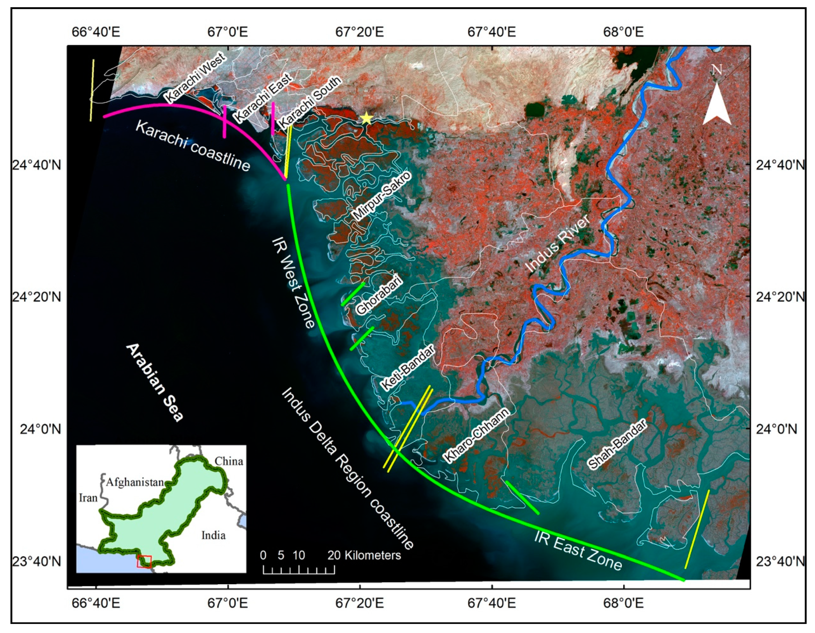
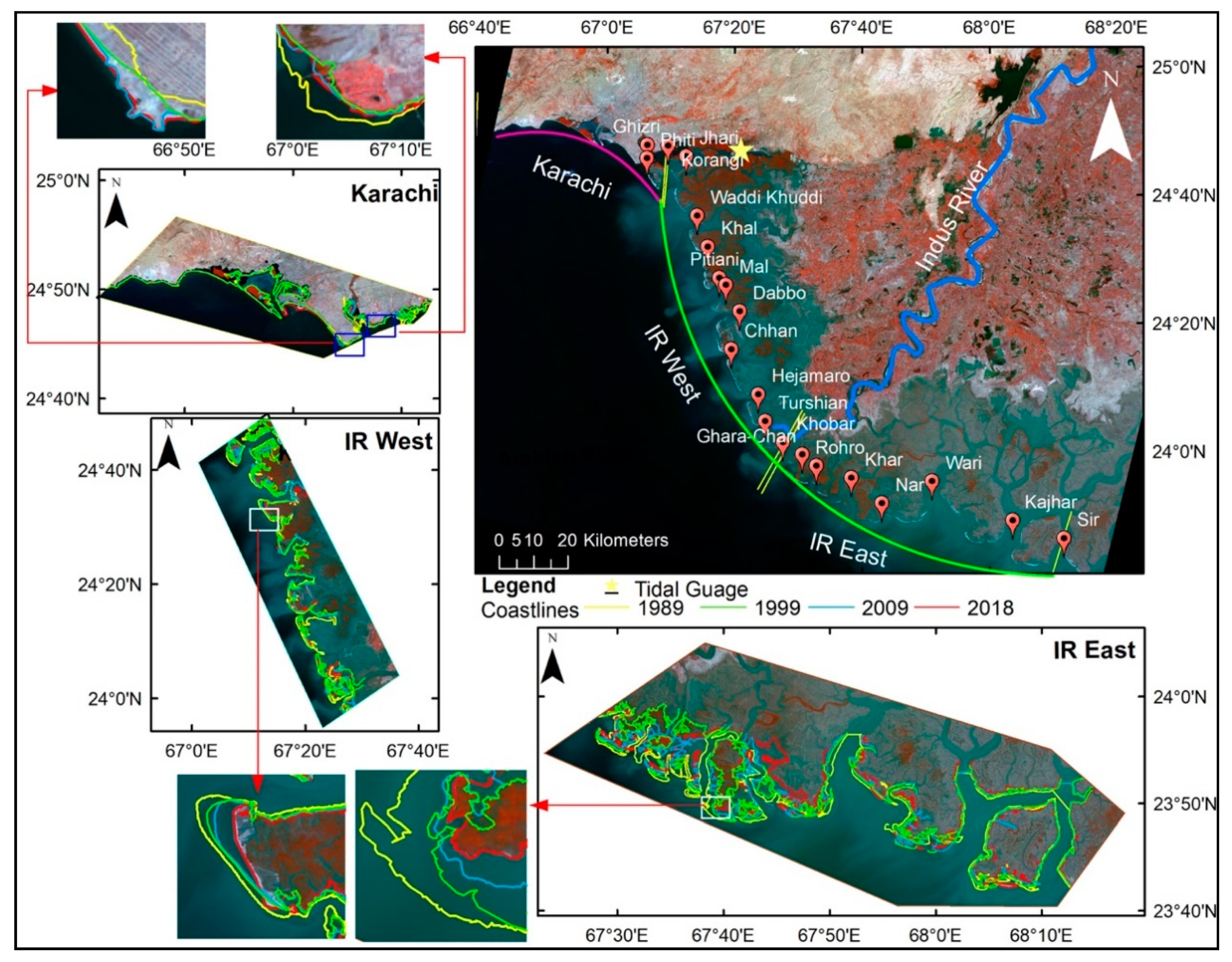
2. Area of Study
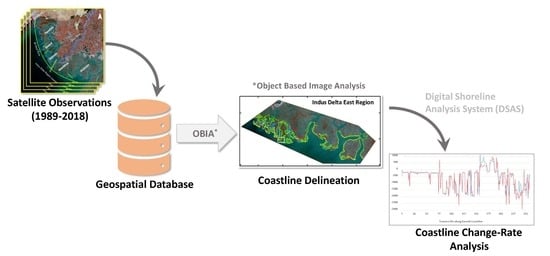
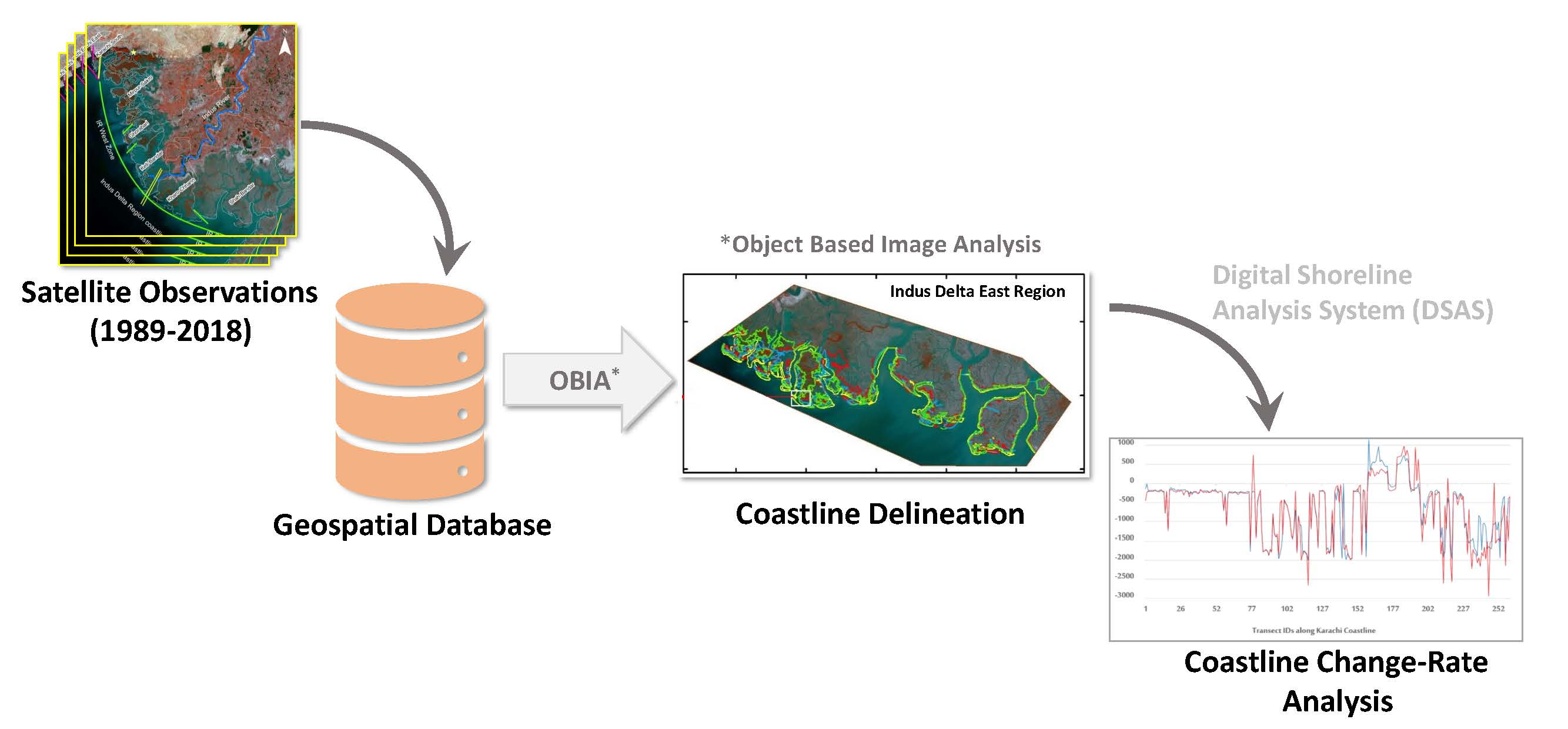
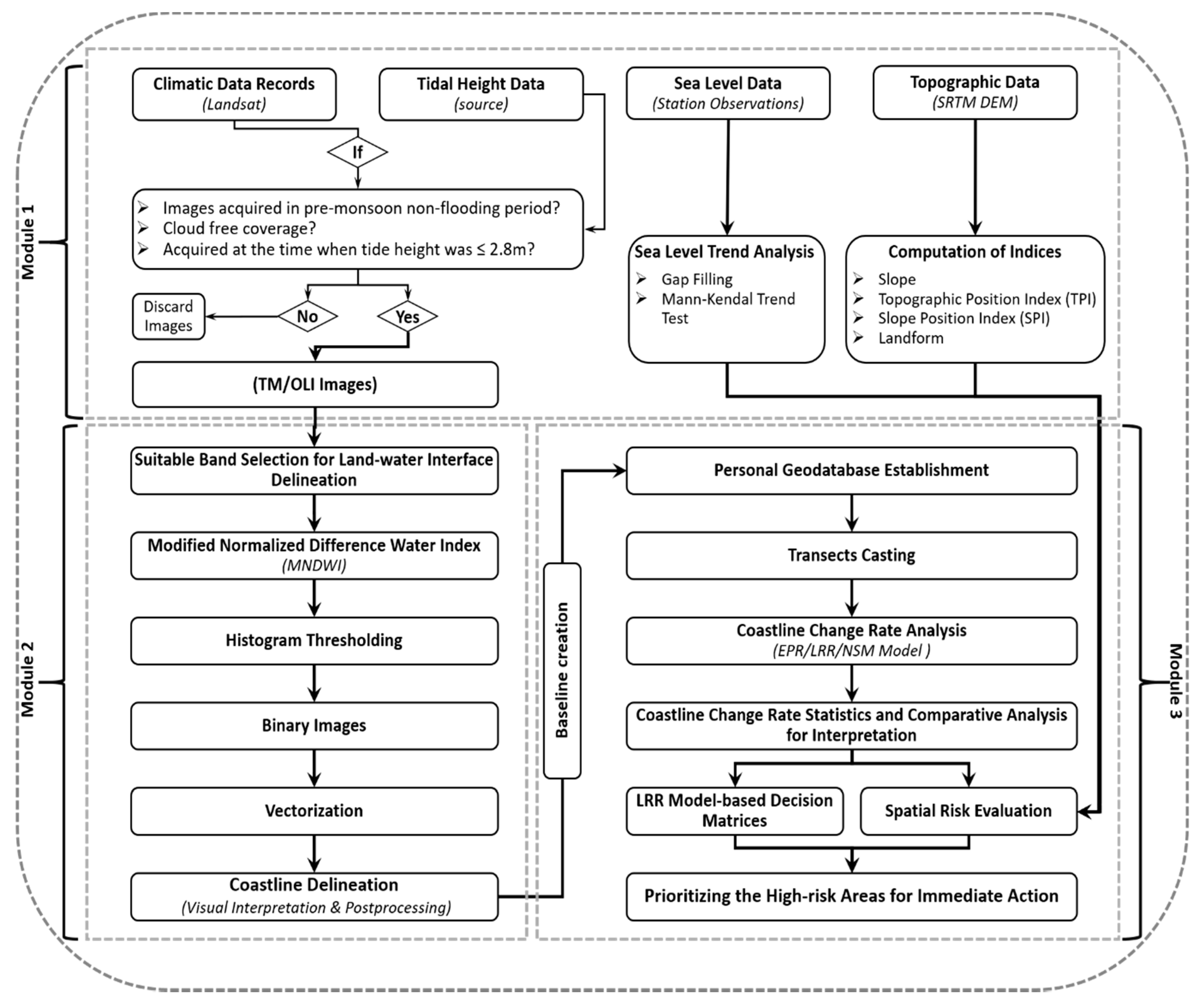
3. Materials and Methods
3.1. Data Set for Coastline Delineation
3.2. Data Set for Coastline Delineation
3.2.1. Coastline Delineation
3.2.2. Analysis of Coastline Change
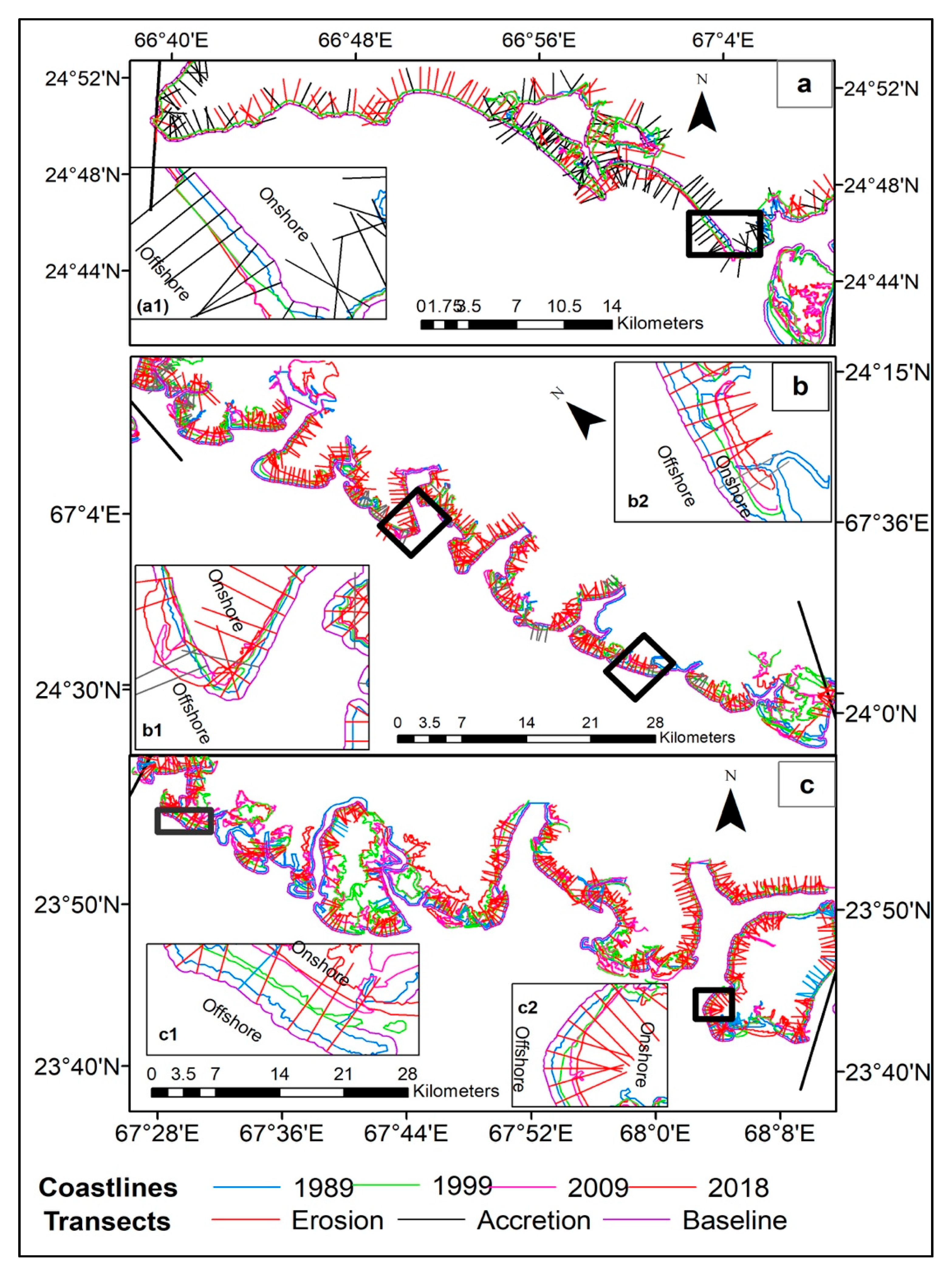
3.2.3. Classification of Erosion
3.2.4. Influencing Factors for Coastline Change
4. Results and Discussion
4.1. Coastline Delineation
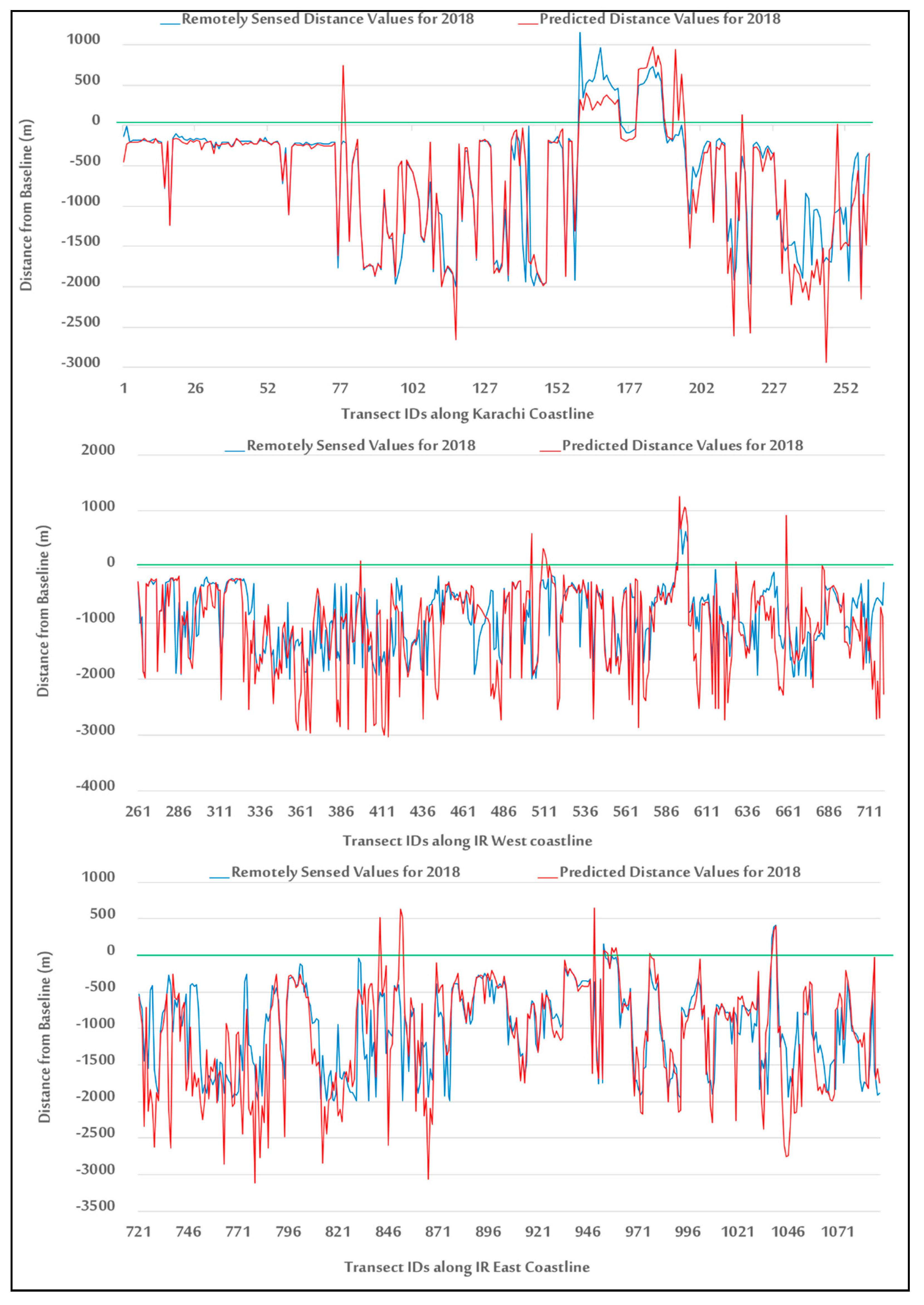
4.2. Analysis of the Rate of Coastline Change
4.3. Coastline Change Rate Statistics during the Last Three Decades (1989–2018)
4.4. Zone-Wise Coastline Change Rate by LRR Model
4.4.1. Karachi Coastline
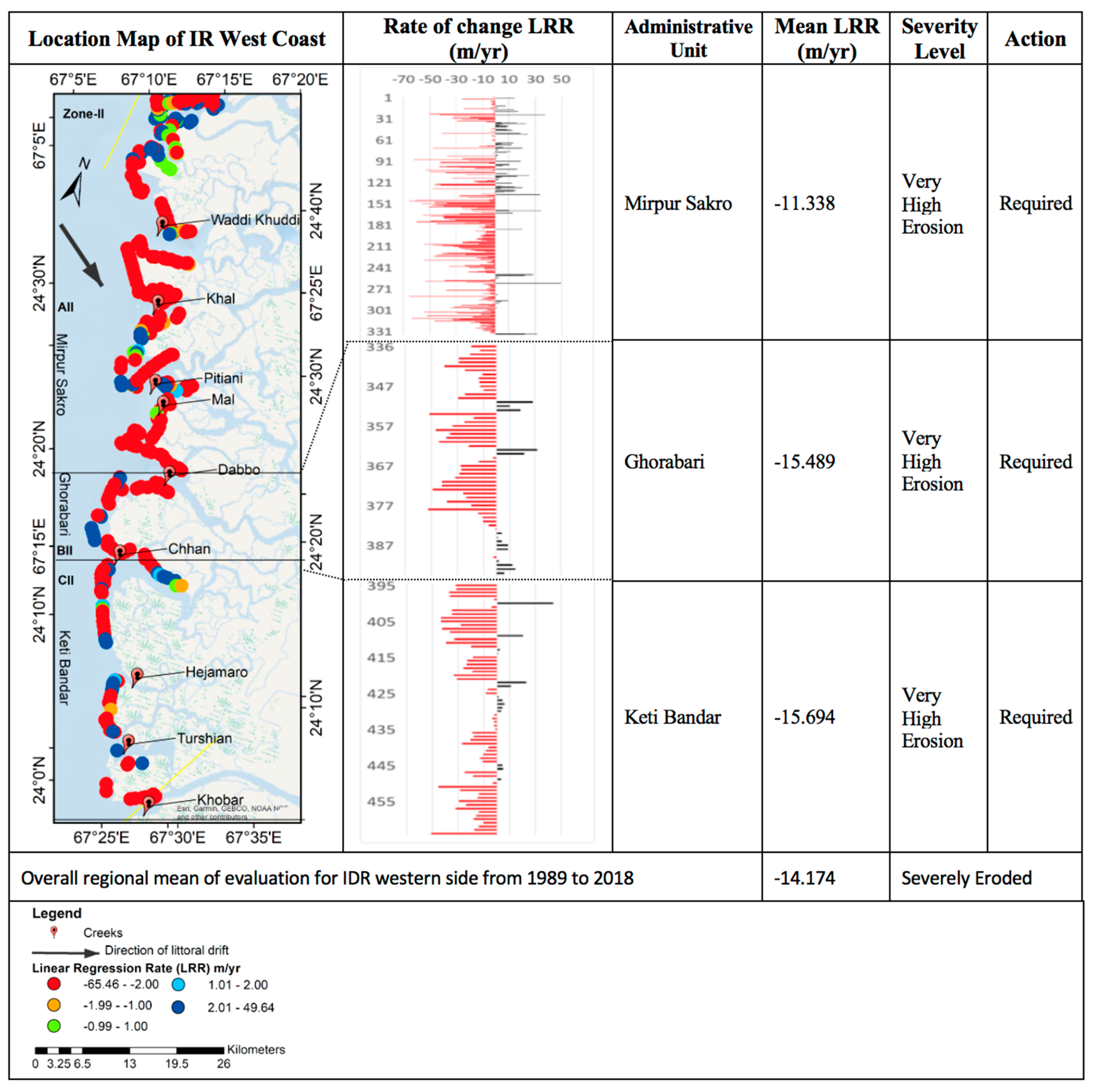
4.4.2. IR West Zone
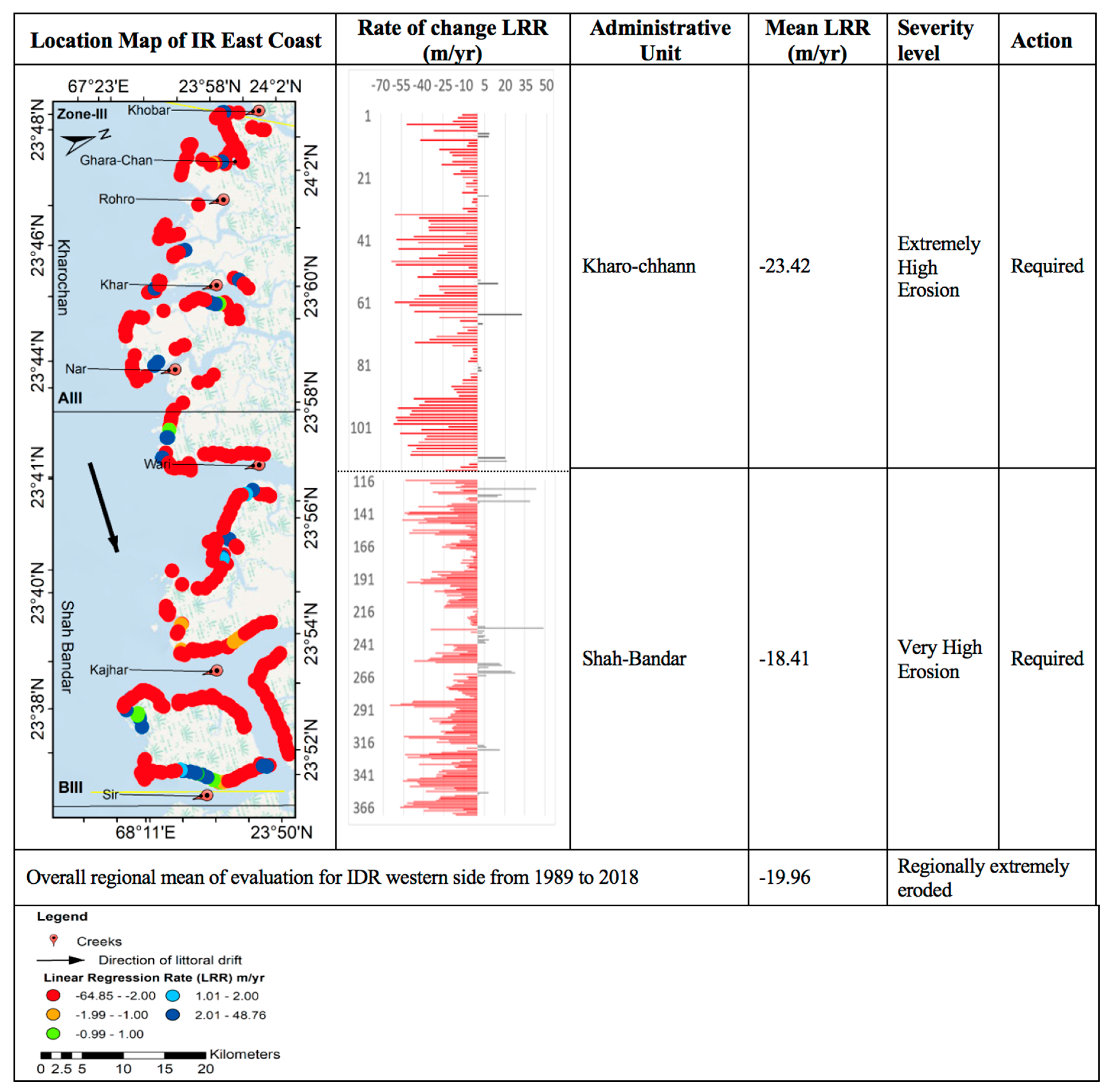
4.4.3. IR East Zone
4.5. Analysis of Influencing Factors of Coastline Change
4.6. Implications for Coastal Sustainability in Pakistan
4.7. Limitations and the Way Forward
5. Conclusions
Supplementary Materials
Author Contributions
Funding
Acknowledgments
Conflicts of Interest
References
- Martínez, C.; Contreras-López, M.; Winckler, P.; Hidalgo, H.; Godoy, E.; Agredano, R. Coastal erosion in central Chile: A new hazard? Ocean Coast. Manag. 2018, 156, 141–155. [Google Scholar] [CrossRef]
- Narra, P.; Coelho, C.; Sancho, F. Multicriteria GIS-based estimation of coastal erosion risk: Implementation to Aveiro sandy coast, Portugal. Ocean Coast. Manag. 2019, 178, 104845. [Google Scholar] [CrossRef]
- Cazenave, A.; Le Cozannet, G. Sea level rise and its coastal impacts. Earth’s Future 2014, 2, 15–34. [Google Scholar] [CrossRef]
- Rahmstorf, S. Rising hazard of storm-surge flooding. Proc. Natl. Acad. Sci.USA 2017, 114, 11806–11808. [Google Scholar] [CrossRef] [PubMed]
- Pollard, J.; Spencer, T.; Brooks, S. The interactive relationship between coastal erosion and flood risk. Prog. Phys. Geogr. Earth Environ. 2018, 43, 0309133318794498. [Google Scholar] [CrossRef]
- Deepika, B.; Avinash, K.; Jayappa, K. Shoreline change rate estimation and its forecast: Remote sensing, geographical information system and statistics-based approach. Int. J. Environ. Sci. Technol. 2014, 11, 395–416. [Google Scholar] [CrossRef]
- UNEP Finance Initiative. The Materiality of Climate Change: How Finance Copes with the Ticking Clock; UNEP Finance Initiative: Geneve, Switzerland, 2009. [Google Scholar]
- Ghosh, M.K.; Kumar, L.; Roy, C. Monitoring the coastline change of Hatiya Island in Bangladesh using remote sensing techniques. ISPRS J. Photogramm. Remote Sens. 2015, 101, 137–144. [Google Scholar] [CrossRef]
- Klein, R.J.; Nicholls, R.J.; Ragoonaden, S.; Capobianco, M.; Aston, J.; Buckley, E.N. Technological options for adaptation to climate change in coastal zones. J. Coast. Res. 2001, 17, 531–543. [Google Scholar]
- Petropoulos, G.P.; Kalivas, D.P.; Griffiths, H.M.; Dimou, P.P. Remote sensing and GIS analysis for mapping spatio-temporal changes of erosion and deposition of two Mediterranean river deltas: The case of the Axios and Aliakmonas rivers, Greece. Int. J. Appl. Earth Obs. Geoinf. 2015, 35, 217–228. [Google Scholar] [CrossRef]
- Xu, N. Detecting Coastline Change with All Available Landsat Data over 1986–2015: A Case Study for the State of Texas, USA. Atmosphere 2018, 9, 107. [Google Scholar] [CrossRef]
- Griffiths, D.; House, C.; Rangel-Buitrago, N.; Thomas, T. An assessment of areal and transect-based historic shoreline changes in the context of coastal planning. J. Coast. Conserv. 2019, 23, 315–330. [Google Scholar] [CrossRef]
- Hein, C.J.; Fallon, A.R.; Rosen, P.; Hoagland, P.; Georgiou, I.Y.; FitzGerald, D.M.; Morris, M.; Baker, S.M.; Marino, G.B.; Fitzsimons, G.; et al. Shoreline dynamics along a developed river mouth barrier island: Multi-decadal cycles of erosion and event-driven mitigation. Front. Earth Sci. 2019, 7, 103. [Google Scholar] [CrossRef]
- Mentaschi, L.; Vousdoukas, M.I.; Pekel, J.F.; Voukouvalas, E.; Feyen, L. Global long-term observations of coastal erosion and accretion. Sci. Rep. 2018, 8, 12876. [Google Scholar] [CrossRef] [PubMed]
- Oost, A.; Hoekstra, P.; Wiersma, A.; Flemming, B.; Lammerts, E.; Pejrup, M.; Hofstede, J.; Van der Valk, B.; Kiden, P.; Bartholdy, J.; et al. Barrier island management: Lessons from the past and directions for the future. Ocean Coast. Manag. 2012, 68, 18–38. [Google Scholar] [CrossRef]
- Rahman, M.M.; Sultana, K.R.; Hoque, M.A. Suitable sites for urban solid waste disposal using GIS approach in Khulna city, Bangladesh. Proc. Pak. Acad. Sci. 2008, 45, 11–22. [Google Scholar]
- Frihy, O.; El-Sayed, M. Vulnerability risk assessment and adaptation to climate change induced sea level rise along the Mediterranean coast of Egypt. Mitig. Adapt. Strateg. Glob. Chang. 2013, 18, 1215–1237. [Google Scholar] [CrossRef]
- Nassar, K.; Mahmod, W.E.; Fath, H.; Masria, A.; Nadaoka, K.; Negm, A. Shoreline change detection using DSAS technique: Case of North Sinai coast, Egypt. Mar. Georesources Geotechnol. 2019, 37, 81–95. [Google Scholar] [CrossRef]
- Kalivas, D.; Kollias, V.; Karantounias, G. A GIS for the assessment of the spatio-temporal changes of the Kotychi Lagoon, Western Peloponnese, Greece. Water Resour. Manag. 2003, 17, 19–36. [Google Scholar] [CrossRef]
- Krestenitis, Y.N.; Kombiadou, K.D.; Androulidakis, Y.S. Interannual variability of the physical characteristics of North Thermaikos Gulf (NW Aegean Sea). J. Mar. Syst. 2012, 96, 132–151. [Google Scholar] [CrossRef]
- Mallinis, G.; Emmanoloudis, D.; Giannakopoulos, V.; Maris, F.; Koutsias, N. Mapping and interpreting historical land cover/land use changes in a Natura 2000 site using earth observational data: The case of Nestos delta, Greece. Appl. Geogr. 2011, 31, 312–320. [Google Scholar] [CrossRef]
- Cui, B.L.; Li, X.Y. Coastline change of the Yellow River estuary and its response to the sediment and runoff (1976–2005). Geomorphology 2011, 127, 32–40. [Google Scholar] [CrossRef]
- Li, X.; Damen, M.C. Coastline change detection with satellite remote sensing for environmental management of the Pearl River Estuary, China. J. Mar. Syst. 2010, 82, 54–61. [Google Scholar] [CrossRef]
- Giosan, L.; Constantinescu, S.; Clift, P.D.; Tabrez, A.R.; Danish, M.; Inam, A. Recent morphodynamics of the Indus delta shore and shelf. Cont. Shelf Res. 2006, 26, 1668–1684. [Google Scholar] [CrossRef]
- Ijaz, M.W.; Mahar, R.B.; Ansari, K.; Siyal, A.A. Optimization of salinity intrusion control through freshwater and tidal inlet modifications for the Indus River Estuary. Estuar. Coast. Shelf Sci. 2019, 224, 51–61. [Google Scholar] [CrossRef]
- Ijaz, M.W.; Mahar, R.B.; Siyal, A.A.; Anjum, M.N. Geospatial analysis of creeks evolution in the Indus Delta, Pakistan using multi sensor satellite data. Estuar. Coast. Shelf Sci. 2018, 200, 324–334. [Google Scholar] [CrossRef]
- Waqas, M.; Nazeer, M.; Shahzad, M.I.; Zia, I. Spatial and Temporal Variability of Open-Ocean Barrier Islands along the Indus Delta Region. Remote Sens. 2019, 11, 437. [Google Scholar] [CrossRef]
- Fatima, H.; Arsalan, M.H.; Khalid, A.; Marjan, K.; Kumar, M. Spatio-temporal analysis of shoreline changes along Makran Coast using remote sensing and geographical information system. In Proceedings of the Fourth International Conference on Space Science and Technology (ICASE), Islamabad, Pakistan, 2–4 September 2015. [Google Scholar]
- Khan, T.M.A.; Razzaq, D.; Chaudhry, Q.U.Z.; Quadir, D.A.; Kabir, A.; Sarker, M.A. Sea level variations and geomorphological changes in the coastal belt of Pakistan. Mar. Geod. 2002, 25, 159–174. [Google Scholar] [CrossRef]
- Siddiqui, M.; Maajid, S. Monitoring of geomorphological changes for planning reclamation work in coastal area of Karachi, Pakistan. Adv. Space Res. 2004, 33, 1200–1205. [Google Scholar] [CrossRef]
- Khan, T.M.A.; Rabbani, M. Sea Level Monitoring and Study of Sea Level Variations along Pakistna Coast: A Component of Integrated Coastal Zone Management; National Institute of Oceanography: Karachi, Pakistan, 2000. [Google Scholar]
- Limmer, D.R.; Henstock, T.J.; Giosan, L.; Ponton, C.; Tabrez, A.R.; Macdonald, D.I.; Clift, P.D. Impacts of sediment supply and local tectonics on clinoform distribution: The seismic stratigraphy of the mid Pleistocene-Holocene Indus Shelf. Mar. Geophys. Res. 2012, 33, 251–267. [Google Scholar] [CrossRef]
- Syvitski, J.P.; Kettner, A.J.; Overeem, I.; Hutton, E.W.; Hannon, M.T.; Brakenridge, G.R.; Day, J.; Vörösmarty, C.; Saito, Y.; Giosan, L. Sinking deltas due to human activities. Nat. Geosci. 2009, 2, 681. [Google Scholar] [CrossRef]
- Schaap, D.; Schmitt, T. EMODnet High Resolution Seabed Mapping-further developing a high resolution digital bathymetry for European seas. In Proceedings of the EGU General Assembly Conference Abstracts, Vienna, Austria, 7–10 April 2019. [Google Scholar]
- Ozturk, D.; Sesli, F.A. Shoreline change analysis of the Kizilirmak Lagoon Series. Ocean Coast. Manag. 2015, 118, 290–308. [Google Scholar] [CrossRef]
- Caldwell, P.; Merrifield, M.; Thompson, P. Sea level measured by tide gauges from global oceans–the Joint Archive for Sea Level holdings (NCEI Accession 0019568), Version 5.5, NOAA National Centers for Environmental Information, Dataset. Cent. Environ. Inf. Dataset 2015, 10, V5V40S47W. [Google Scholar]
- Toure, S.; Diop, O.; Kpalma, K.; Maiga, A.S. Shoreline Detection using Optical Remote Sensing: A Review. ISPRS Int. J. Geo-Inf. 2019, 8, 75. [Google Scholar] [CrossRef]
- Pardo-Pascual, J.; Sánchez-García, E.; Almonacid-Caballer, J.; Palomar-Vázquez, J.; Priego De Los Santos, E.; Fernández-Sarría, A.; Balaguer-Beser, Á. Assessing the accuracy of automatically extracted shorelines on microtidal beaches from Landsat 7, Landsat 8 and Sentinel-2 Imagery. Remote Sens. 2018, 10, 326. [Google Scholar] [CrossRef]
- Liu, H.; Wang, L.; Sherman, D.J.; Wu, Q.; Su, H. Algorithmic foundation and software tools for extracting shoreline features from remote sensing imagery and LiDAR data. J. Geogr. Inf. Syst. 2011, 3, 99. [Google Scholar] [CrossRef]
- Paravolidakis, V.; Ragia, L.; Moirogiorgou, K.; Zervakis, M. Automatic coastline extraction using edge detection and optimization procedures. Geosciences 2018, 8, 407. [Google Scholar] [CrossRef]
- Alesheikh, A.A.; Ghorbanali, A.; Nouri, N. Coastline change detection using remote sensing. Int. J. Environ. Sci. Technol. 2007, 4, 61–66. [Google Scholar] [CrossRef]
- Armenio, E.; De Serio, F.; Mossa, M. Analysis of data characterizing tide and current fluxes in coastal basins. Hydrol. Earth Syst. Sci. 2017, 21, 3441. [Google Scholar] [CrossRef]
- Nandi, S.; Ghosh, M.; Kundu, A.; Dutta, D.; Baksi, M. Shoreline shifting and its prediction using remote sensing and GIS techniques: A case study of Sagar Island, West Bengal (India). J. Coast. Conserv. 2016, 20, 61–80. [Google Scholar] [CrossRef]
- Gornitz, V.M.; Daniels, R.C.; White, T.W.; Birdwell, K.R. The development of a coastal risk assessment database: Vulnerability to sea-level rise in the US Southeast. J. Coast. Res. 1994, 327–338. [Google Scholar]
- Mahapatra, M.; Ramakrishnan, R.; Rajawat, A. Coastal vulnerability assessment of Gujarat coast to sea level rise using GIS techniques: A preliminary study. J. Coast. Conserv. 2015, 19, 241–256. [Google Scholar] [CrossRef]
- Jenness, J. Topographic Position Index (Tpi_jen. Avx) Extension for ArcView 3. x, v. 1.3 a. Jenness Enterprises. 2006. Available online: http://www.jennessent.com/arcview/tpi (accessed on 18 December 2019).
- Mann, H.B. Nonparametric tests against trend. Econom. J. Econom. Soc. 1945, 13, 245–259. [Google Scholar] [CrossRef]
- Siddig, N.A.; Al-Subhi, A.M.; Alsaafani, M.A. Tide and mean sea level trend in the west coast of the Arabian Gulf from tide gauges and multi-missions satellite altimeter. Oceanologia 2019, 61, 401–411. [Google Scholar] [CrossRef]
- Sen, P.K. Estimates of the regression coefficient based on Kendall’s tau. J. Am. Stat. Assoc. 1968, 63, 1379–1389. [Google Scholar] [CrossRef]
- Taibi, H.; Haddad, M. Estimating trends of the Mediterranean Sea level changes from tide gauge and satellite altimetry data (1993–2015). J. Oceanol. Limnol. 2019, 37, 1–10. [Google Scholar] [CrossRef]
- Dolan, R.; Fenster, M.S.; Holme, S.J. Temporal analysis of shoreline recession and accretion. J. Coast. Res. 1991, 7, 723–744. [Google Scholar]
- Douglas, B.C.; Crowell, M. Long-term shoreline position prediction and error propagation. J. Coast. Res. 2000, 16, 145–152. [Google Scholar]
- Maiti, S.; Bhattacharya, A.K. Shoreline change analysis and its application to prediction: A remote sensing and statistics based approach. Mar. Geol. 2009, 257, 11–23. [Google Scholar] [CrossRef]
- Sengupta, D.; Chen, R.; Meadows, M.E. Building beyond land: An overview of coastal land reclamation in 16 global megacities. Appl. Geogr. 2018, 90, 229–238. [Google Scholar] [CrossRef]
- Luijendijk, A.; Hagenaars, G.; Ranasinghe, R.; Baart, F.; Donchyts, G.; Aarninkhof, S. The state of the world’s beaches. Sci. Rep. 2018, 8, 6641. [Google Scholar] [CrossRef]
- Kanwal, S.; Ding, X.; Zhang, L. Measurement of Vertical Deformation in Karachi Using Multi-Temporal Insar. In Proceedings of the IGARSS 2018-2018 IEEE International Geoscience and Remote Sensing Symposium, Valencia, Spain, 22–27 July 2018; pp. 1395–1398. [Google Scholar]
- Hashmi, S.; Ahmad, S. GIS-Based Analysis and Modeling of Coastline Erosion and Accretion along the Coast of Sindh Pakistan. J. Coast. Zone Manag. 2018, 21, 6–9. [Google Scholar] [CrossRef]
- Pakistan, I. Mangroves of Pakistan, Status and Management; International Union for Conservation of Nature: Gland, Switzerland, 2005. [Google Scholar]
- Mukhtar, I.; Hannan, A. Constrains on mangrove forests and conservation projects in Pakistan. J. Coast. Conserv. 2012, 16, 51–62. [Google Scholar] [CrossRef]
- WWF-Pakistan. GIS/RS Based Monitoring of Indus Delta, A Half Century Comparison; WWF: Morges, Switzerland, 2010. [Google Scholar]
- Milliman, J.; Haq, B.U. Sea-Level Rise and Coastal Subsidence: Causes, Consequences, and Strategies; Springer Science & Business Media: Berlin, Germany, 1996; Volume 2. [Google Scholar]
- Inam, A.; Clift, P.D.; Giosan, L.; Tabrez, A.R.; Tahir, M.; Rabbani, M.M.; Danish, M. The geographic, geological and oceanographic setting of the Indus River. In Large Rivers: Geomorphology and Management; John Wiley & Sons, Ltd.: Chichester, UK, 2007; pp. 333–345. [Google Scholar] [CrossRef]
- Jelgersma, S.; Van der Zijp, M.; Brinkman, R. Sealevel rise and the coastal lowlands in the developing world. J. Coast. Res. 1993, 9, 958–972. [Google Scholar]
- Weeman, K.; Lynch, P. New Study Finds Sea Level Rise Accelerating. 2018. Available online: https://climate.nasa.gov/news/2680/new-study-finds-sea-level-rise-accelerating/ (accessed on 9 September 2019).
- Farah, A.; Meynell, P. Sea Level Rise Possible Impacts on the Indus Delta, Pakistan, IUCN Korangi Ecosystem Project, Paper. 1992.
- Muzaffar, M.; Inam, A.; Hashmi, M.; Mehmood, K.; Zia, I.; Imran Hasaney, S. Climate change and role of anthropogenic impact on the stability of Indus deltaic Eco-region. J. Biodivers. Environ. Sci. 2017, 10, 164–176. [Google Scholar]
- Van Slobbe, E.; de Vriend, H.J.; Aarninkhof, S.; Lulofs, K.; de Vries, M.; Dircke, P. Building with Nature: In search of resilient storm surge protection strategies. Nat. Hazards 2013, 66, 1461–1480. [Google Scholar] [CrossRef]
- Sajjad, M.; Li, Y.; Tang, Z.; Cao, L.; Liu, X. Assessing hazard vulnerability, habitat conservation, and restoration for the enhancement of mainland China’s coastal resilience. Earth’s Future 2018, 6, 326–338. [Google Scholar] [CrossRef]
- Prasetya, G. The role of coastal forests and trees in protecting against coastal erosion. In Proceedings of the Regional Technical Workshop on Coastal Protection in the aftermath of the Indian Ocean tsunami: What role for forest and trees, Khao Lak, Thailand, 28–31 August 2006. [Google Scholar]
- Sebesvari, Z.; Foufoula-Georgiou, E.; Harrison, I.; Brondizio, E.; Bucx, T.; Dearing, J.; Ganguly, D.; Ghosh, T.; Goodbred, S.; Hagenlocher, M.; et al. Imperatives for Sustainable Delta Futures. In Brief for GSDR; Sustainable Development Knowledge Platform: New York, NY, USA, 2016. [Google Scholar]


| Zone | Administrative Units |
|---|---|
| Karachi | Karachi West, Karachi South, and Karachi East |
| IR West | Mirpur Sakro, Ghorabari, and Keti Bandar, located between Korangi Creek and Khobar Creek |
| IR East | Kharo-Chhann and Shah Bandar, located between Ghara-Chan Creek and Sir Creek |
| Dataset | Description | Processing Level | Spatial and Temporal Resolution | Source | |||
|---|---|---|---|---|---|---|---|
| Pixel Size | Acquisition Time (UTC) | Acquisition Date | Tidal Height | ||||
| Satellite Images | TM | Level 2 | 30 m | 05:26:11 | 3 April 1989 | 1.90 m | US Geological Survey (https://espa.cr.usgs.gov/) |
| 30 m | 05:41:59 | 6 April 1999 | 2.5 m | ||||
| 30 m | 05:44:13 | 10 April 2009 | 0.1 m | ||||
| OLI | 30 m | 05:56:49 | 2 March 2018 | 2.80 m | |||
| Ocean Data | Mean Tide Level | - | 1989–2018 | Tides 4 Fishing (https://tides4fishing.com/) | |||
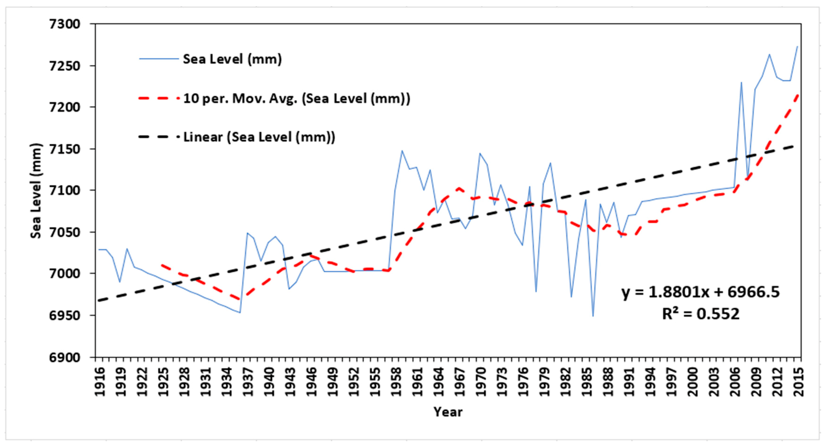
| Mean Sea Level Data | - | 1916–2015 | Permanent Service for Mean Sea Level (PSMSL) [36] | ||||
| Topography | Shuttle Radar Topography Mission (SRTM) | - | 30 m | Open-Topography (http://opentopo.sdsc.edu/datasets) | |||
| Zone | Karachi Zone | IR West Zone | IR East Zone | |||||
|---|---|---|---|---|---|---|---|---|
| Subzone | Karachi West | Karachi South | Karachi East | Mirpur Sakro | Keti-Bandar | Ghorabari | Kharo-Chhann | Shah-Bandar |
| No. of transects | 128 | 69 | 13 | 385 | 122 | 137 | 106 | 272 |
| Mean accretion rate (+) | 4.01 | 12.14 | 9.37 | 11.49 | 7.87 | 11.53 | 10.72 | 11.88 |
| Mean erosion rate (−) | −4.17 | −6.09 | −13.95 | −19.98 | −20.04 | −19.57 | −27.46 | −23.37 |
| Min accretion rate (+) | 0.00 | 0.28 | 0.00 | 0.02 | 0.12 | 0.12 | 0.46 | 0.01 |
| Max erosion rate (−) | −74.59 | −48.86 | −57.22 | −72.66 | −52.35 | −65.46 | −62.36 | −64.85 |
| Max accretion rate (+) | 48.26 | 53.61 | 51.09 | 62.04 | 43.64 | 51.09 | 32.17 | 48.76 |
| Min erosion rate (−) | −0.02 | −0.05 | −0.20 | −0.11 | −0.25 | −0.25 | −1.30 | −0.41 |
| Zonal average | −0.85 ± 0.45 | −14.17 ± 0.55 | −19.96 ± 0.65 | |||||
| Category | Low Erosion | Severe Erosion | Severe Erosion | |||||
| Creek | Min | Max | Mean | Zone | Creek | Min | Max | Mean | Zone |
|---|---|---|---|---|---|---|---|---|---|
| Waddi | −15.33 | −0.25 | −8.91 | IR West | Ghara-Chan | −17.36 | −3.01 | −4.01 | IR East |
| Khal | −54.50 | −1.40 | −17.51 | IR West | Khar | −46.21 | 32.17 | −14.98 | IR East |
| Pitiani | −65.46 | −0.85 | −9.48 | IR West | Nar | −53.55 | 21.00 | −13.34 | IR East |
| Dabbo | −46.12 | −26.90 | −15.39 | IR West | Wari | −57.32 | 8.09 | −31.62 | IR East |
| Chhan | −52.35 | −2.14 | −26.82 | IR West | Kajhar | −64.50 | −4.13 | −26.48 | IR East |
| Turshian | −25.28 | 4.61 | −8.13 | IR West | Sir | −34.66 | −8.76 | −3.14 | IR East |
| Khobar | −51.33 | −11.08 | −22.22 | IR West /IR East | |||||
© 2019 by the authors. Licensee MDPI, Basel, Switzerland. This article is an open access article distributed under the terms and conditions of the Creative Commons Attribution (CC BY) license (http://creativecommons.org/licenses/by/4.0/).
Share and Cite
Kanwal, S.; Ding, X.; Sajjad, M.; Abbas, S. Three Decades of Coastal Changes in Sindh, Pakistan (1989–2018): A Geospatial Assessment. Remote Sens. 2020, 12, 8. https://doi.org/10.3390/rs12010008
Kanwal S, Ding X, Sajjad M, Abbas S. Three Decades of Coastal Changes in Sindh, Pakistan (1989–2018): A Geospatial Assessment. Remote Sensing. 2020; 12(1):8. https://doi.org/10.3390/rs12010008
Chicago/Turabian StyleKanwal, Shamsa, Xiaoli Ding, Muhammad Sajjad, and Sawaid Abbas. 2020. "Three Decades of Coastal Changes in Sindh, Pakistan (1989–2018): A Geospatial Assessment" Remote Sensing 12, no. 1: 8. https://doi.org/10.3390/rs12010008
APA StyleKanwal, S., Ding, X., Sajjad, M., & Abbas, S. (2020). Three Decades of Coastal Changes in Sindh, Pakistan (1989–2018): A Geospatial Assessment. Remote Sensing, 12(1), 8. https://doi.org/10.3390/rs12010008