Cross-Comparison and Methodological Improvement in GPS Tomography

Abstract

GPS tomography has been investigated since 2000 as an attractive tool for retrieving the 3D field of water vapour and wet refractivity. However, this observational technique still remains a challenging task that requires improvement of its methodology. This was the purpose of this study, and for this, GPS data from the Australian Continuously Operating Research Station (CORS) network during a severe weather event were used. Sensitivity tests and statistical cross-comparisons of tomography retrievals with independent observations from radiosonde and radio-occultation profiles showed improved results using the presented methodology. The initial conditions, which were associated with different time-convergence of tomography inversion, play a critical role in GPS tomography. The best strategy can reduce the normalised root mean square (RMS) of the tomography solution by more than 3 with respect to radiosonde estimates. Data stacking and pseudo-slant observations can also significantly improve tomography retrievals with respect to non-stacked solutions. A normalised RMS improvement up to 17% in the 0–8 km layer was found by using 30 min data stacking, and RMS values were divided by 5 for all the layers by using pseudo-observations. This result was due to a better geometrical distribution of mid- and low-tropospheric parts (a 30% coverage improvement). Our study of the impact of the uncertainty of GPS observations shows that there is an interest in evaluating tomography retrievals in comparison to independent external measurements and in estimating simultaneously the quality of weather forecasts. Finally, a comparison of multi-model tomography with numerical weather prediction shows the relevant use of tomography retrievals to improving the understanding of such severe weather conditions.

1. Potential of GPS Tomography for Meteorological Applications

Global Positioning System (GPS) tomography considers the use of slant-integrated estimates, wet delays, or corresponding water vapour content estimated from the data records of ground-based GPS stations to respectively retrieve the 3D field of wet refractivity or water vapour density, as introduced by [1,2]. Comparisons of tomography retrievals with other techniques (e.g., those using a water vapour radiometer, radiosonde, raman lidar, or atmospheric emitted radiance interferometer) and with numerical weather models have shown relevant results and an encouraging understanding of meteorological situations ([3,4,5,6,7,8,9,10,11,12,13,14,15,16,17]) The resolution and configuration/geometry of the network of GPS stations are critical parameters with which to obtain the best scenario for applying GPS tomography to retrieve water vapour density or wet refractivity. These fields can be ideally retrieved for meteorological applications with a horizontal resolution of a few kilometres, a vertical resolution of ~500 m in the lower troposphere, and a vertical resolution of ~2 km in the upper troposphere, with a time resolution of 15 to 5 min. However, to obtain this remarkable geometrical resolution, data from a dense homogeneously distributed network of GPS stations (e.g., a network with 5–25 km spacing) are required, ideally with stations at different altitudes (with a range of a few hundred meters) according to the orography [18,19,20].

The description of the humidity field, especially the flux of water vapour in the lower atmosphere, is essential for the understanding of convective meteorological events by forecasters and the quantitative prediction of precipitation [21]. Looking at GPS tomography, the limitations and reliability of retrievals can be linked to two main hurdles. The first limitation is the geometry and resolution of the grid adjusted by the inversion process. This is directly linked to the resolution of the network of stations considered. Note that Bender et al. [22] have shown that minor improvements can be expected by combining GPS (US Global Positioning System), GLONASS (GLObal NAvigation Satellite System of Russian government), and Galileo (EU global satellite-based navigation system) observations, especially for the volume pixels (so called voxels) of the lower troposphere. The second limitation, deeply linked to the lack of geometrical distribution and representativeness of retrievals, concerns the convergence of the inversion process to a reliable solution. Improvements of the tomographic method, with the aim to obtain the best convergence of retrievals, have been developed by [23] using singular value decomposition combined with a Kalman filter. Improvements have also been developed by Bender et al. [13] with algebraic reconstruction, by Perler et al. [14] with the use of new parametrised approaches, and more recently by Rohm [24] with an unconstrained approach and the use of a robust Kalman filter [25], and by Zhao et al. [26] by considering various input observation weighting schemes. Note that for all these methods, the observation-a priori weighting scheme affects the inversion process, and the redundancy or the conflict of information from GPS slant observations crossing the same voxel are critical for good achievement of the tomography technique. Currently, methodological improvements are still needed to face these two limitations in the GNSS (Global Navigation Satellite System) tomography processes.

The structure of this manuscript is as follows. The next section describes the selected meteorological situation used when applying our new methodology. Section 3 presents a description of the GPS data and independent observations considered. Section 4 characterises the five tomography models of this study (i.e., the setting used in calculations, the algorithm of convergence processes, the approach used to constrain the a priori condition and the weight attributed to the data, and the intrinsic specificity of each model and their quality controls). Section 5 presents the methodology suggested for use to face the limitations of GNSS tomography. Section 6 shows results of improved GPS tomography retrievals and the interest in using sensitivity tests in meteorological applications. Section 7 presents a cross-comparison of tomography models with profiles from external observations. Finally, the last section summarises and highlights conclusions and perspectives for future works.

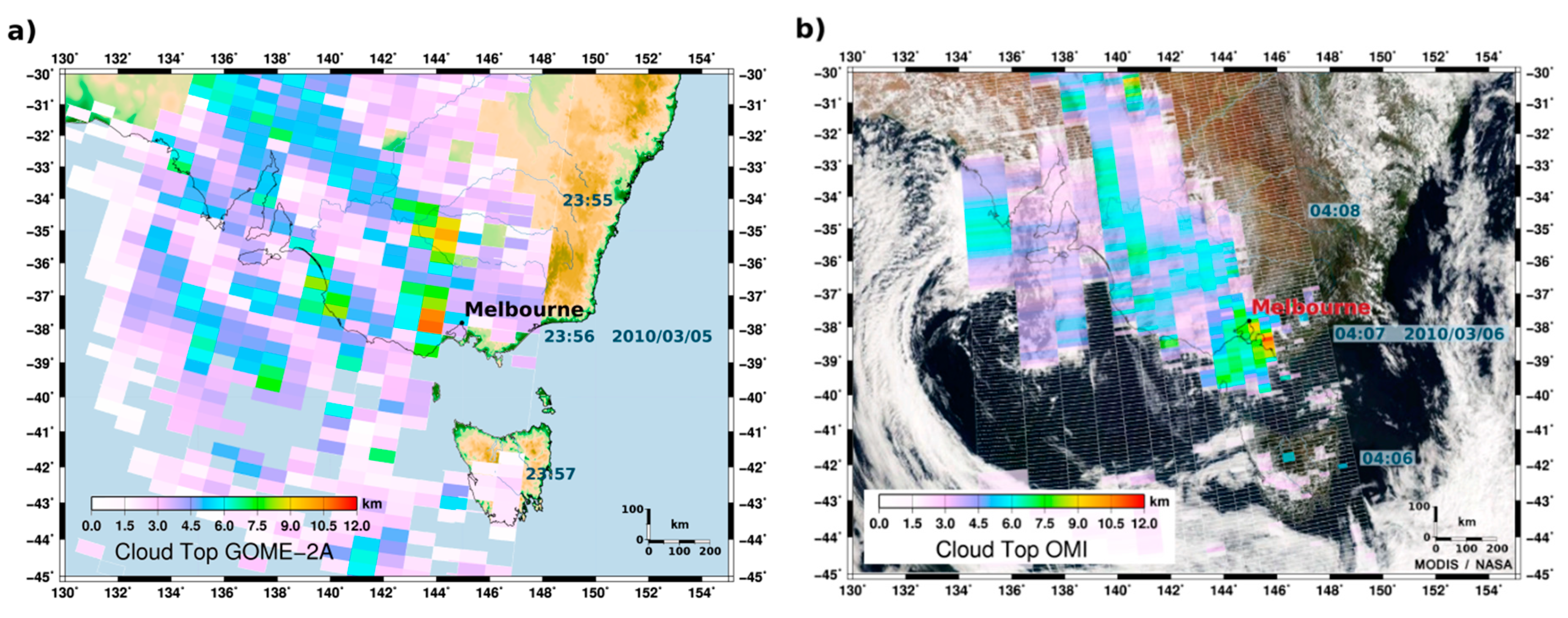
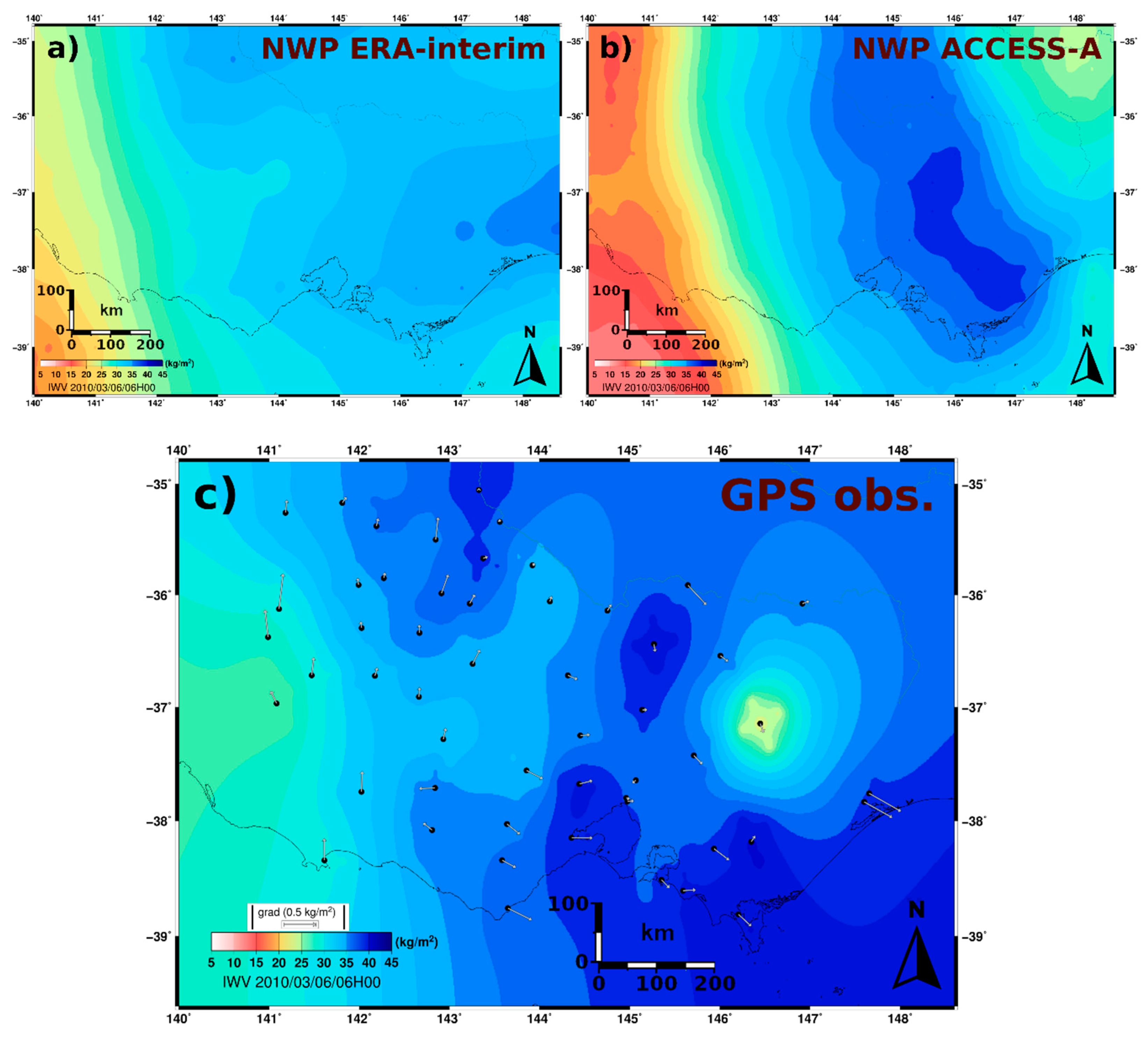
2. Overview of the Selected Severe Weather Situation

Although the pattern of Australia’s rainfall accumulation is one of the lowest on Earth, mainly due to the fact that deserts cover slightly more than half of the surface of this country, heavy rainfall can take place seasonally, i.e., in the northern equatorial region, which has a tropical climate, and in the southern sub-tropical region, which has a with temperate climate. This study focusses on torrential rainfall, which happens occasionally during the autumn season in the southeastern Australian Victoria region, and more specifically on the meteorological situation of the March 2010 Melbourne storm.

Heavy rainfall affected the state of Victoria from 6 to 8 March, 2010, and caused consequent flash floods that disrupted the life of the population of the greater Melbourne region, with several injuries and damages resulting [27]. This event was probably the most severe of the past decade for this region [28]. Such an event, acting as a mesoscale convective system (MCS) with a horizontal extension of generally over 10 km, a long life-time (sometimes of a few hours), and a strong vertical vorticity, largely caused by wind shear, is called a supercell storm. The mean monthly precipitation of Melbourne (50 mm) fell in only one day (61 mm on 6 March, 2010), including hailstones with a size of up to 5 cm, as reported by the Australian Bureau of Meteorology [29]. Considering estimations of cloud top altitudes from Global Ozone Monitoring Experiment–2 (GOME-2) and Ozone Monitoring Instrument (OMI) sensors, a vertical extension which was at least higher than 10 km was induced close to Melbourne by a supercell storm and can be observed in Figure 1. Cloud top altitudes were evaluated using cloud top pressure retrievals [30,31] combined with the assumption of an atmosphere in a hydrostatic equilibrium. This application of hypsometric equations required inputs of ground pressure and mean temperature of the column of air for each footprint considered. These two parameters were obtained from the outputs of the analysis of the Australian Community Climate and Earth-System Simulator (ACCESS-A), with a focus on Australian area, and the operational Numerical Weather Prediction (NWP) of the Australian Bureau of Meteorology [32]. Figure 1a,b show the cloud top altitudes obtained by GOME-2 and OMI during the overpass over Melbourne at 23:56 UTC (on 5 March, 2010) and 04:07 UTC (on 6 March, 2010), respectively. In Figure 1a, the MCS (with a vertical extension of over 9 km) covers an area of 80 × 80 km² (the size of a pixel from the GOME-2 instrument is 80 × 40 km²), and the area with stratiform precipitation (with a vertical extension of over 6 km) is about 160 × 160 km².

In Figure 1b, convective precipitation with a high vertical extension can be seen to concern an area of about 24 × 84 km² (a pixel from OMI is 24 × 13 km²) and stratiform precipitation in an area of 168 × 195 km². The background of Figure 1b is an image (visible channel) from the Moderate Resolution Imaging Spectroradiometer (MODIS). This imager, on board the Aqua satellite, simultaneously looks at the same area of the Earth as OMI/Aura. The dimension of the MCS detected by GOME-2 and OMI are respectively confirmed by heavy and moderate precipitation recorded by the weather radar of Melbourne; see Choy et al. [27] and Manning et al. [33] for more details regarding this meteorological situation.

A typical configuration of the atmosphere with instability in the troposphere (e.g., that triggered by the topography or due to low level convergence) associated with the opposition of dry and moist air was required to initiate deep convection during the 6–8 March superstorm of greater Melbourne [27]. At the end of the day on 5 March, 2010 (UTC time), the lifting of moist air coming from the south and southeast sides of Melbourne and warm dry air coming from westwards of Melbourne triggered the convection. The water vapour content of the troposphere is a key parameter which initiates and keeps running deep convection. Its monitoring is critical to evaluating the severity of severe weather events (nowcasting) and to forecasting meteorological situations. Figure 2 shows the 2D field of integrated water vapour (IWV) from ACCESS-A NWP during the supercell storm of Melbourne in March 2010. Even a horizontal resolution of ACCESS-A outputs of 12 km, the weather prediction used in this study, was not sufficient to properly forecast this storm and the creation of such a supercell. Strong differences with the IWV fields from GPS are observed in Figure 2 (see Section 3.1 for more details regarding estimates of water vapour content from GPS).

The flux of water vapour from the south of Melbourne is indicated by horizontal IWV gradients (Figure 2c), aligned along south north in a southeast–northwest direction in the central section of Victoria and north south in the west part of Victoria. These opposite gradients illustrate the critical condition that took place in the region surrounding Melbourne which maintained a convective process inside the supercell. Note that IWV gradients were obtained using a $\mathsf{\kappa }$ conversion factor [34] (see Equation (6)) applied on wet gradients (see Equation (4)). Monitoring by GPS techniques using a dense network can be essential for improving the capability to better understand and forecast such events. For this purpose, this study focusses on testing five different types of tomography software for estimating reliable tomography retrievals.

3. GPS Data and External Observations

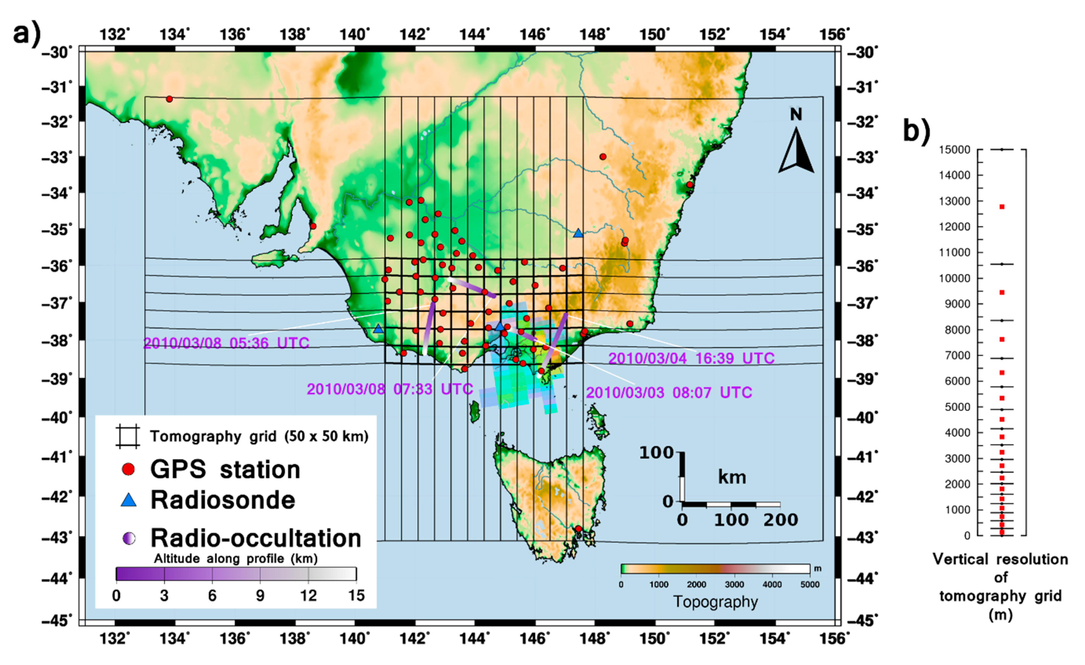
3.1. Data Inputs for GPS Tomography Using the Continuously Operating Reference Station (CORS) Network

During the Melbourne storm in March 2010, 69 stations of the Victorian GPS CORS network were recording signals emitted from 31 GPS satellites. The locations of these stations are presented in Figure 3a. The GPS data were processed by the Royal Melbourne Institute of Technology University using the double difference technique with Bernese 5.0 software [35]. The full details of the processing strategy are available in a paper by Rohm et al. [36]. The data used in this study were derived using the “shortest baselines network solution” with the following parameters: precise final International GNSS Service (IGS) orbits in an IGS05 reference frame with an L3/L5 strategy, minimum constraints applied on the translation parameters for Helmert transformation based on IGS fiducial stations, elevation dependent weighting, and a 5°-cutoff angle. Zenith total delays of the neutral atmosphere (ZTDs) had relative constraints applied and were estimated in 30 min steps with gradients modelled by tilting every 6 h. The GMF mapping function [37] is employed for geodetic software analysis and retrievals of tropospheric parameters. Hence, ZTDs and horizontal delay gradients $\overrightarrow{G}=\left(G_{NS},G_{EW}\right)$ were retrieved every 30 min (a piece-wise linear function was evaluated every 30 min) covering the period from 3 March, 2010 to 10 March, 2010.

The understanding of meteorological situations by using GPS tomography techniques can rely on retrieving the 3D fields of wet refractivity and water vapour density. Initial GPS tropospheric parameters are converted into slant wet delays (SWDs) and slant-integrated Water Vapour contents (SIWVs) to retrieve, respectively, these fields. Estimates of ground pressure and mean temperature (of the column) are required for each station of the GPS CORS network. These parameters were obtained using outputs from the ACCESS-A weather model. The ground pressures and temperatures of the four surrounding ACCESS-A grid points of a GPS station were converted to the altitude of the GPS site (using a hypsometric equation and linear vertical interpolation, respectively). Then, pressures and temperatures at the location of the GPS site were obtained using bi-linear horizontal interpolation. This strategy is best in the absence of a collocated meteorological station [38]. A time interpolation was also applied from 6 h of a weather model to a 30 min time resolution of GPS tropospheric parameters. The formula of Saastamoinen [39] was used to convert pressure data into zenith hydrostatic delay (ZHD). The zenith wet delay (ZWD) was obtained by simply subtracting ZHD from ZTD estimates (i.e., ZWD = ZTD − ZHD). Using the field of ground pressure from ACCESS-A, the hydrostatic part of the azimuthal contribution of GPS gradient to delays to slant delays was removed to allow only the wet contribution to remain [40,41].

The elevation ($є$) and azimuth (α) dependency of the SWD is described by an isotropic (${\mathrm{L}}_{\mathrm{sym}}^{\mathrm{wet}}$) and anisotropic (${\mathrm{L}}_{\mathrm{az}}^{\mathrm{wet}}$) component in Equation (1).

$$\mathrm{SWD}={\mathrm{L}}_{\mathrm{sym}}^{\mathrm{wet}}(є)+{\mathrm{L}}_{\mathrm{az}}^{\mathrm{wet}}\left(є,\mathsf{\alpha }\right)$$

(1)

The isotropic SWD (${\mathrm{L}}_{\mathrm{sym}}^{\mathrm{wet}}$) is obtained by mapping of the ZWD using a wet mapping function ${\mathrm{mf}}_{\mathrm{sym}}^{\mathrm{wet}}$ (in our case GMF from [37]) in the direction of the GPS satellite in a view above 5° elevation (Equation (2)).

$${\mathrm{L}}_{\mathrm{sym}}^{\mathrm{wet}}(є)=\mathrm{ZWD}·{\mathrm{mf}}_{\mathrm{sym}}^{\mathrm{wet}}(є)$$

(2)

The first order wet anisotropic contribution (${\mathrm{L}}_{\mathrm{az}}^{\mathrm{wet}}$) is formulated in Equation (3).

$${\mathrm{L}}_{\mathrm{az}}^{\mathrm{wet}}\left(є,\mathsf{\alpha }\right)={\mathrm{mf}}_{\mathrm{az}}^{\mathrm{wet}}\left(є,\mathrm{C}\right)·\left(G_{\mathrm{NS}}^{\mathrm{wet}}·\cos \left(\alpha \right)+G_{\mathrm{EW}}^{\mathrm{wet}}·\sin \left(\alpha \right)\right)$$

(3)

This equation uses a gradient mapping function $\left({\mathrm{mf}}_{\mathrm{az}}^{\mathrm{wet}}=1/\left(\sin є\tan є+\mathrm{C}\right)\right)$ which depends on the satellite’s elevation and on a constant ($\mathrm{C}$ = 0.0032) ([42,43]), and the gradient wet components ($G_{\mathrm{NS}}^{\mathrm{wet}}$,$G_{\mathrm{EW}}^{\mathrm{wet}}$) in the north–south and east–west direction, which are multiplied with the cosine or sine of the azimuth ($\alpha$), respectively. Note that the one-way residual has not been considered in the ${\mathrm{L}}_{\mathrm{az}}^{\mathrm{wet}}$ and SWD retrievals here.

The gradient components ($G_{NS}$,$G_{EW}$) retrieved by GPS technique describe the total asymmetric effect. This means there is no distinction between wet and hydrostatic gradients [1,43]. However, the wet gradient component can be expressed by the difference of the hydrostatic to the total component, i.e.,

$$\left(\begin{array}{c}{G}_{\mathrm{NS}}^{\mathrm{wet}}\\ G_{\mathrm{EW}}^{\mathrm{wet}}\end{array}\right)=\left(\begin{array}{c}{G}_{NS}\\ G_{EW}\end{array}\right)-\left(\begin{array}{c}{G}_{\mathrm{NS}}^{\mathrm{hydrostatic}}\\ G_{\mathrm{EW}}^{\mathrm{hydrostatic}}\end{array}\right)$$

(4)

To obtain the hydrostatic gradient components ($G_{\mathrm{NS}}^{\mathrm{hydrostatic}}$ and $G_{\mathrm{EW}}^{\mathrm{hydrostatic}}$), a characterisation of the surface pressure field around each GPS station is required. In that case, the hydrostatic gradient can be established by fitting a plane through the pressure measurements [40,41]. The spatial variations of the hydrostatic delay per unit of distance (km) in the north–south ($Z_{\mathrm{NS}}^{\mathrm{hydrostatic}}$) and east–west ($Z_{\mathrm{EW}}^{\mathrm{hydrostatic}}$) directions can be calculated from the pressure field for each GPS site. Surface pressure measurements around all GPS stations of the CORS network were not available during the supercell storm of 6–8 March 2010. For this reason, the pressure field of ACCESS-A NWP was considered. Assuming an exponential law in the hydrostatic refractivity and considering the scale height of the gradients in the hydrostatic delays as being set to $H$ = 13 km, as suggested by [43], the spatial variations of the hydrostatic delay can be converted into hydrostatic gradients [1,44,45], i.e.,

$$\left(\begin{array}{c}{G}_{\mathrm{NS}}^{\mathrm{hydrostatic}}\\ G_{\mathrm{EW}}^{\mathrm{hydrostatic}}\end{array}\right)=H.\left(\begin{array}{c}{Z}_{\mathrm{NS}}^{\mathrm{hydrostatic}}\\ Z_{\mathrm{EW}}^{\mathrm{hydrostatic}}\end{array}\right)$$

(5)

The resulting slant wet delays $\left(\mathrm{SWD}={\int }^{}{N}_{w}ds\right)$ are used as inputs for GPS tomography to retrieve 3D fields of wet refractivity $\left(N_w\right)$. $ds$ is the differential distance along the slant path travel of the GPS signal. The second type of slant measurements used is water vapour slant total column density, also called slant-integrated water vapour contents, which can be simply obtained from SWDs by multiplication with factor $\mathsf{\kappa }$, as shown in Equation (6). Then, GPS tomography retrieves the 3D field of water vapour density (${\rho }_{wv}$).

$$\mathrm{SIWV}=\mathsf{\kappa }\mathrm{SWD}={{\displaystyle \int }}^{}{\rho }_{wv}ds$$

(6)

The expression of the $\mathsf{\kappa }$ factor [34] requires an estimation of the mean temperature of the column of air (T_m) above the GPS station. Hence, temperature profiles from ACCESS-A were interpolated in space and time. The obtained $\mathsf{\kappa }$ factors were applied in Equation (6) for the conversion of SWDs into SIWVs.

From 3 March, 2010 to 10 March, 2010 (288 epochs, 30 min time resolution), in total, 197429 pairs of SWDs/SIWVs were retrieved (about 686 pairs at each time). These observations were the basis input data for our tomography and sensitivity tests.

3.2. Independent Observations of Water Vapour Density and Wet Refractivity Profiles

3.2.1. Profiles from Radiosonde

The most common and accurate technique used to measure the vertical profile of temperature, pressure, dew point temperature, and wind speed and direction is a sensor attached to an automatic radio-sounding balloon released either every 6, 12, or at a minimum 24 h. Usually, profiles reach up to 30 km and have a very high vertical resolution; a major drawback of such measurements is the horizontal movement of the balloon as it ascents vertically due to winds. The ascent time is around 1 h. In 2010 in Australia there were 32 radiosonde stations with only one located in Victoria (Melbourne airport–YMML) and another two within a short distance from the Victorian border (Wagga Wagga–YSWG and Mount Gambier–YMMG), as shown in Figure 3. Only the YMML radiosonde station, located at an altitude of 141 m and position of (37.67°S, 144.83°E), has been considered. This radiosonde (YMML–RS) data was available twice a day (at noon and midnight) for all days used in the study. The radiosonde technique is highly accurate for observations of the troposphere with a 1–2 hPa accuracy for pressure, 0.5 °C accuracy for temperature, and 5% accuracy for relative humidity [46]. Based on the radiosonde data, the following calculations were made to retrieve wet refractivity and water vapour content: (1) the formula used by Sargent [47] was applied to obtain the relative humidity from the dew point temperature [48]; (2) the formula used by Sonntag [49] was used to calculate the partial pressure of water vapour $p_w$ from $RH$ and $T$; and (3) the atmospheric state parameters $p_w$, $p$, and $T$ were used to calculate wet refractivity $N_w$ and water density profiles ${\rho }_{wv}$ using equations proposed by Davis et al., [50], i.e.,

$$N=k_1{R}_d\rho +{k^{\prime }}_2\frac{p_w}{T}+k_3\frac{p_w}{T^2}$$

(7)

where $k_1,{k^{\prime }}_2$, and $k_3$ denote empirically-derived refractivity coefficients, $R_d$ is a gas constant for dry air, and $\rho$ is the atmospheric density.

3.2.2. Profiles from the Radio-Occultation Technique

The radio-occultation (RO) profiles used in this study are wet profiles which were acquired via the Constellation Observing System for Meteorology, Ionosphere, and Climate (COSMIC) and re-processed in 2013 at the COSMIC Data Analysis Archive Center (CDAAC). The wet profile (wetPrf) is an interpolated product with a vertical resolution of 100 m which was obtained using a one-dimensional variational (1DVar) technique together with European Centre Medium Weather Forecast (ECMWF) low resolution analysis data, and it contains latitude and longitude of the perigee point, pressure, temperature (T), water vapour pressure ($p_w$), refractivity, and a mean sea level altitude of the perigee point. The atmospheric parameters were computed using a 1DVar approach where refractivity is weighted in such a way that the temperature is basically the same as the dry temperature in regions where the water vapour is insignificant [51]. Analyses of specific humidity estimated by GPS RO [52] have shown consistency of being within 0.1–0.3 g/kg in the median with Global Climate Observing System (GCOS) Reference Upper-Air Network (GRUAN) radiosonde data and with theoretical studies of accuracy [53,54]. The RO globally performs better than the radiosondes between 5 and 25 km of altitude when compared to the ECMWF global analysis [54].

For a comparison with tomography results, we converted the $p_w$ in ${\rho }_{wv}$ by using the gas equation

$${\rho }_{wv}=\frac{p_w}{461.525\ast T}\ast 1000$$

(8)

for the four COSMIC RO reported in

Table 1. List of Radio-Occultations.

Mean Times of Measurement	Cosmic-GPS Couple	Lower Position	Top of Tomography Grid	Higher Position
3 March, 2010 08:07 UTC	C006-G09	(37.99°S, 145.98°E, 2300 m)	(37.71°S, 145.17°E, 12,800 m)	(37.66°S, 144.62°E, 39,900 m)
4 March, 2010 16:39 UTC	C004-G12	(37.33°S, 147.03°E, 1900 m)	(38.81°S, 146.21°E, 12,800 m)	(37.66°S, 144.62°E, 39,900 m)
8 March, 2010 05:36 UTC	C003-G01	(37.04°S, 142.60°E, 1200 m)	(38.25°S, 142.33°E, 12,800 m)	(38.86°S, 142.35°E, 39,900 m)
8 March, 2010 07:33 UTC	C006-G27	(36.83°S, 144.63°E, 1300 m)	(36.41°S, 143.26°E, 12,800 m)	(36.32°S, 142.52°E, 39,900 m)

and shown in Figure 3.

4. A Selection of Five Tomography Models

GPS tomography uses slant-integrated measurements (SWDs and SIWVs) inside a defined volume to retrieve $N_w$ or ${\rho }_{wv}$ estimates for each voxel N_pqr, as illustrated in Figure 4. For highest consistency, the same GPS data set and the same 3D grid were used for each of the five tomography models considered in this study.

For each GPS station within the voxel model, the integrated slant observations SLANT_GPS (in our case the SWDs or SIWVs) were converted into 3D fields of $N_w\mathrm{or}{\rho }_{wv}$ using Equation (9), i.e.,

$${\mathrm{SLANT}}_{\mathrm{GPS}}\left(\mathrm{P},\mathsf{\alpha },є\right)={\displaystyle \sum }_{i=1}^{N{B}_{vx}}{\mathrm{N}}_{x_i{y}_i{z}_i}\Delta s_i$$

(9)

where P is the position of a GPS station (latitude, longitude, and altitude), є is the elevation and $\mathsf{\alpha }$ the azimuth angle of a GPS satellite, $N{B}_{vx}$ is the number of voxels crossed by each observation, and $\Delta s_i$ is the ray length in each voxel i (x_i $\in$ [1, p], y_i $\in$ [1, q], z_i $\in$ [1, r]). Following this, axes x, y, and z are associated, respectively, with longitude, latitude, and altitude. For the tomographic grid, the horizontal size of the voxels in the inner grid is 0.5° ~50 km (thick black lines in Figure 3a), which is slightly denser than the mean baseline (~70 km) of the GPS network; see preconditions from Bender and Raabe [55]. Twelve voxels are considered longitudinally (p = 12) and six voxels latitudinally (q = 6). All around this inner grid, voxels of the outer grid are considered inside a band with a width of about 400 km (thin black lines of Figure 3a). The outer grid is used to compensate for water vapour contributions outside the tomographic model, and, therefore, keep stations in the solution which are located close to the edge of the inner grid. To deal with the topography under the tomographic grid, note that the lower layer of the grid is at the altitude above the sea level (altitude = 0 m a.s.l.). The voxels for which there is no GPS station inside or under are simply not retrieved by tomography models. Section 6.1 and Table 5 discuss the percentage of voxels retrieved in our calculations according to different types of calculations and settings.

Assuming the hypothesis of straight rays (the bending effect which can affect observations under 15° elevations ([56]) has not been considered in our study), the inversion problem becomes linear. The formulation of the linear inverse problem reads

$$\mathrm{d}=\mathrm{Gm}+{\mathrm{C}}_{\mathrm{D}}$$

(10)

where $\mathrm{d}$ represents the SWD/SIWV observations. This is connected to the model m of wet refractivity/water vapour density ($N_w/{\rho }_{wv}$) (which we want to retrieve) by the geometrical matrix $\mathrm{G}$ and the observation errors defined by the covariance operator ${\mathrm{C}}_{\mathrm{D}}$. Positions of stations and satellites used to characterise the geometrical matrix are expressed in Cartesian coordinates. SWD/SIWV observations are associated with errors (∆SWD/∆SIWV) which are expressed using ${\mathrm{C}}_{\mathrm{D}}$. Positions and observations are the inputs of this inverse problem. The solution m does not exist because GPS tomography is an ill-posed problem. However, the alternative is to find ${\mathrm{m}}^{\prime }$, which minimises the L₂-norm using the minimisation factor ξ, which is expressed as

$$\Vert \mathrm{d}-{\mathrm{Gm}}^{\prime }\Vert {}_{L_2}<\mathsf{\xi }$$

(11)

Different standard techniques exist for solving such linear inverse problems, e.g., singular value decomposition (SVD), truncated singular value decomposition (TSVD), weighted and damped least-square adjustment (LS), Kalman-filter, simultaneous algebraic reconstruction technique (SART), conjugate gradient method, Tikhonov-regularisation, stacking, and double-difference–spline interpolation.

This study uses five models with different inversion techniques, i.e., SVD, TSVD, LS, and SART. Retrievals were obtained mainly in 3D and for one model in 2D (the Technical University of Ostrava (TUO) model), and these were proceeded with for $N_w$ and ${\rho }_{wv}$, except for the Technische Universität Wien (TUW) model ($N_w$ only) and the University of Beira Interior (UBI) model (${\rho }_{wv}$ only).

Table 2. Overview of the five models and retrievals achieved. Legend: BIRA, Royal Belgian Institute for Space Aeronomy; WUELS, Wroclaw University of Environmental and Life Sciences; TUW, Technische Universität Wien; UBI, University of Beira Interior; TUO, Technical University of Ostrava; SVD, singular value decomposition; LS, weighted and damped least-square adjustment; TSVD, truncated singular value decomposition; SART, simultaneous algebraic reconstruction technique; $N_w$, wet refractivity; ${\rho }_{wv}$, water vapour density; RMS, root mean square.

Tomography Model	Inversion	Dim.	Retrievals	Covariance Operator Data	Covariance Operator A Priori Model	Quality Check
BIRA	SVD, weighted and damped LS adjustment	3D	$N_w$, ${\rho }_{wv}$	10%	90%	Resolution matrix, covariance matrix, spread
WUELS	Kalman filter with selective SVD	3D	$N_w$, ${\rho }_{wv}$	Diagonal obs. error fed	Diagonal-height-dependent	Condition number and variance–covariance $N_w$, ${\rho }_{wv}$
TUW	TSVD	3D	$N_w$	Elevation dependent weighting	Altitude-dependent weights	RMS of weighted residuals
UBI	SART	3D	${\rho }_{wv}$	Unit covariance matrix	Unit covariance matrix	Condition number and converge
TUO	LS adjustment	2D	$N_w$, ${\rho }_{wv}$	-	-	-

summarises the characterisation of the covariance operator of data and the a priori model, as well as a the quality check for tomographic retrievals.

More information about the five tomography models can be found in the Appendix A, Appendix B, Appendix C, Appendix D and Appendix E. Note that for all the tomography models and all the tests performed in this study, the same a priori condition ${\mathrm{m}}_0$ was considered. This condition was based on 6 h of NWP outputs from ACCESS-A interpolated to the tomography grid of Figure 3. The reader can take a look at Puri et al. [32] for more details regarding the observations considered in the assimilation chain of ACCESS-A, which is a four-dimensional observation variational assimilation method (4DVAR). In 2010, the radio-occultation observations were not assimilated in the ACCESS-A system.

5. Methodological Improvement in GNSS Tomography

The inverse problem treated by GNSS tomography was ill-posed due to a non-homogenous distribution of slant observations through the 3D grid (lack and redundancy), but it was also ill-conditioned due to the high number of parameters physically embedded. This explains why the stabilisation of the tomographic solution remains a challenging task, in spite of methodological improvements [25]. Two main limitations are currently identified in the methodology of the GNSS tomography technique: (1) the deficiency of geometric representativeness and (2) the problems of convergence related to a reliable solution in the inverse process. The present work looks at the limitation induced by a non-sufficient geometrical distribution of GPS observations (e.g., those due to a network of stations with a mean baseline >30 km) and investigates methods for improving it. This study also investigates the issue in the convergence process of the tomographic inversion, which is linked to geometrical representativeness, and the impact of the observation uncertainty on the quality of tomographic results.

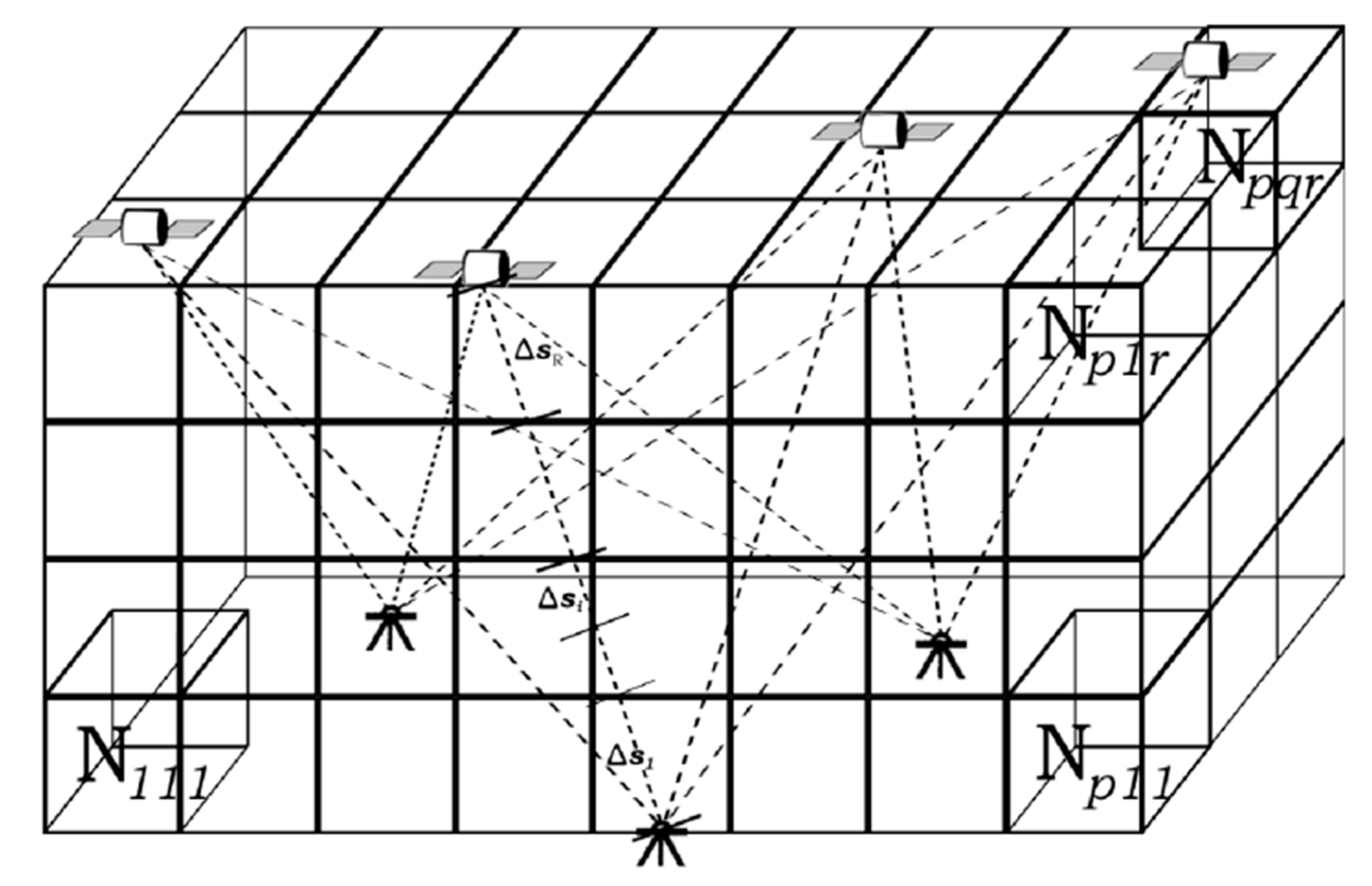
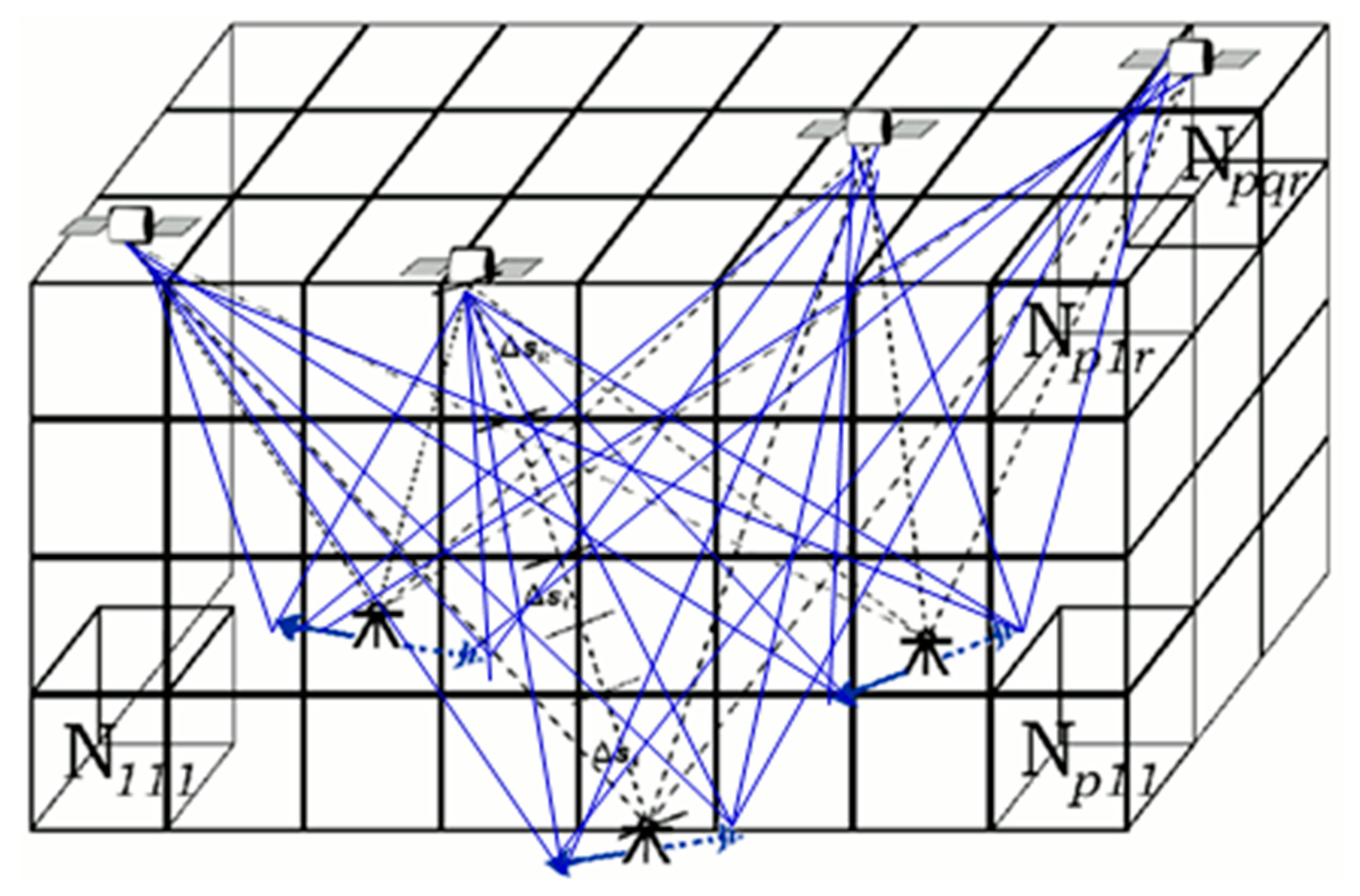
5.1. Methodology for Improving of the Geometrical Representativeness

Two types of improvement of the geometrical distribution of tomography retrievals are suggested and tested, namely, stacking of slant GPS data and additional pseudo-slant observations.

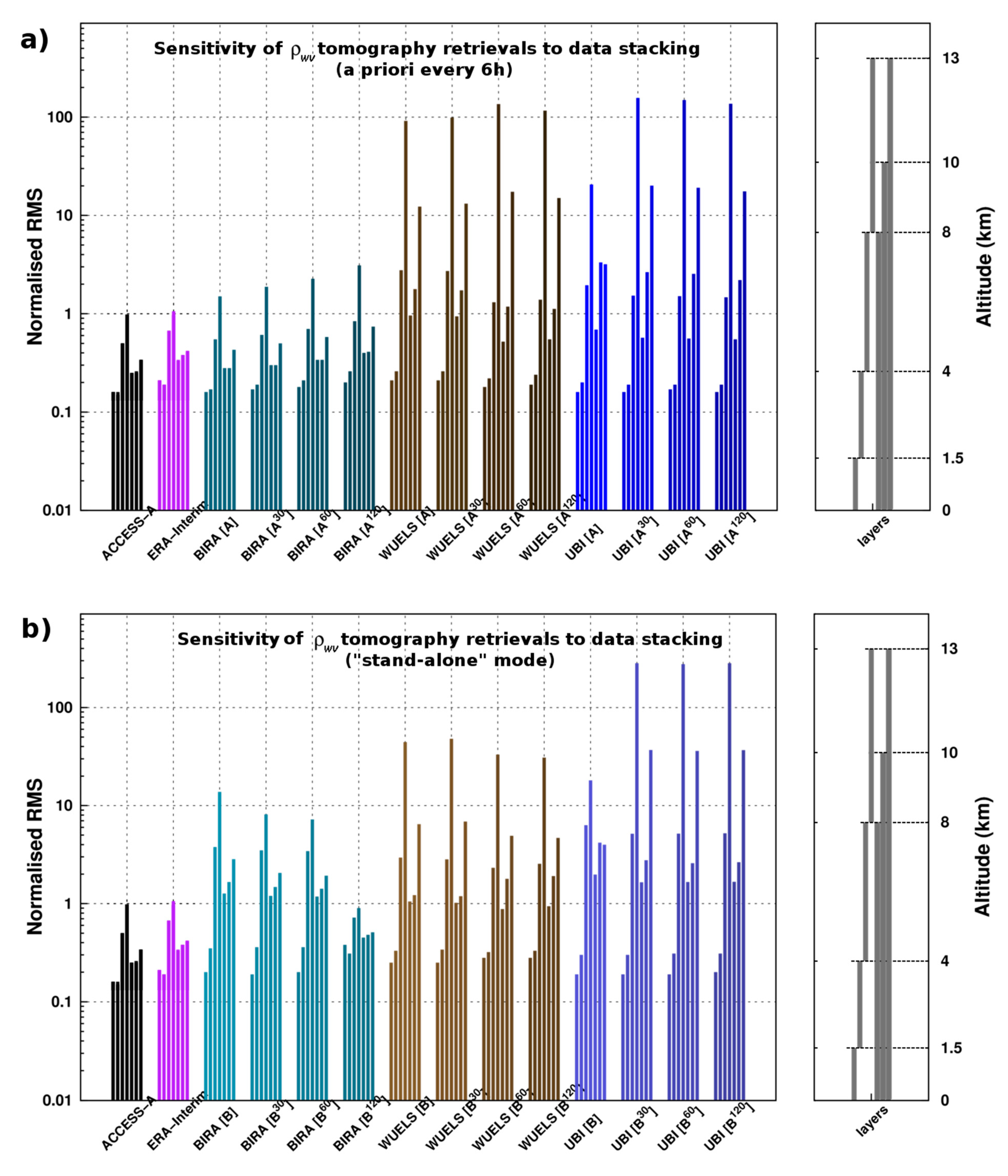
5.1.1. Data Stacking of Slant Observations

The time resolution of the tropopsheric parameters (ZTD and gradients) used to assess the slant observations triggered the increment chosen for the stacking periods, i.e., 30 min. The resolution of our tomography grid (50 km), which was related to the resolution of the GPS network considered, was a limitation to improving the geometrical distribution. In our case, there was no interest in choosing a shorter stacking period (e.g., 15 min). The observation stacking procedure decreases, in theory, the condition number of the design matrix (see Equation (A3) and Equation (A4) in Appendix A) by improving the observation geometry; however, it can also decrease the accuracy of retrieval if the troposphere is active and changes rapidly within the stacking window. Stacking of GPS data (SWD/SIWV) was tested for three stacking periods (30, 60, and 120 min before and after the time of tomography reconstruction).

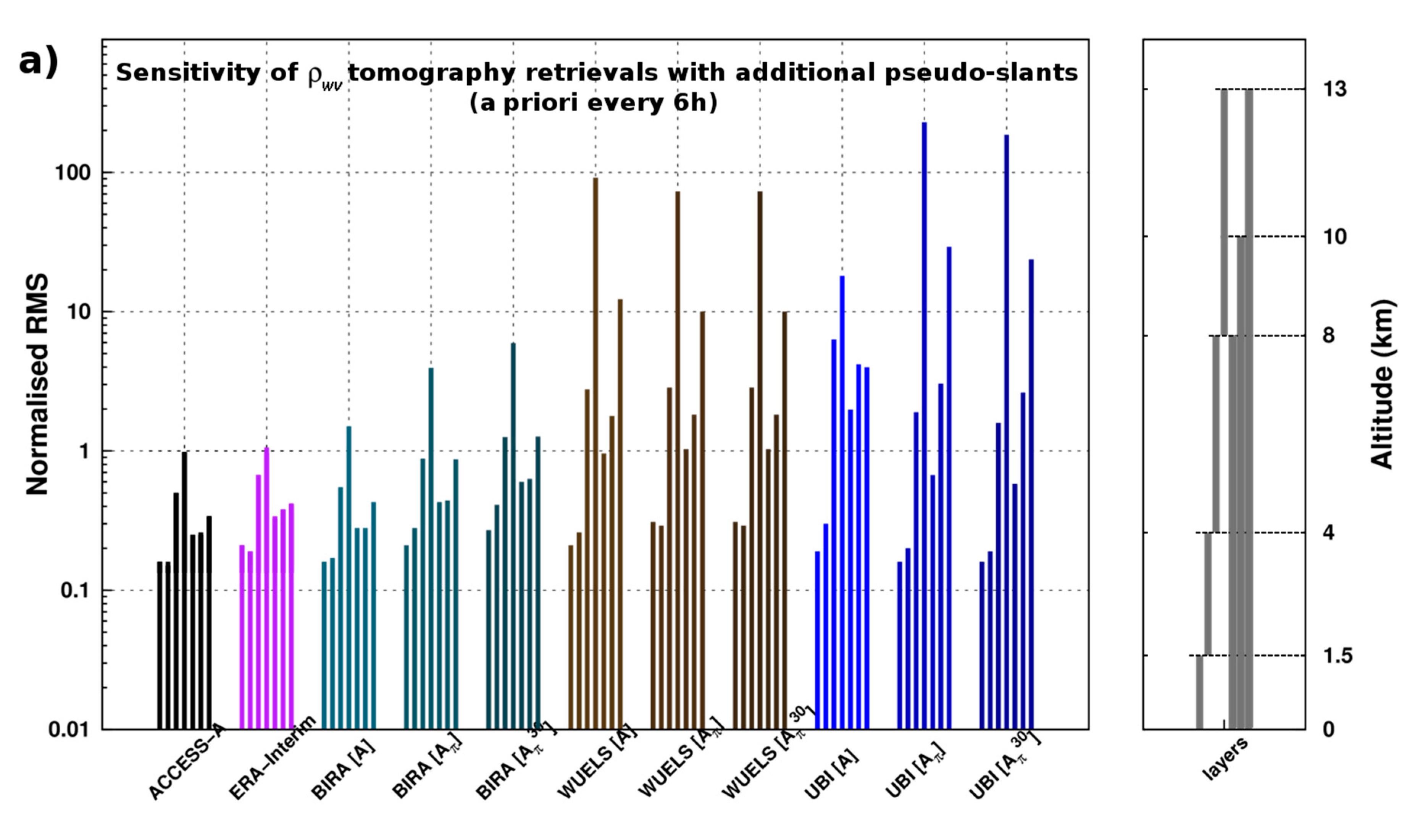
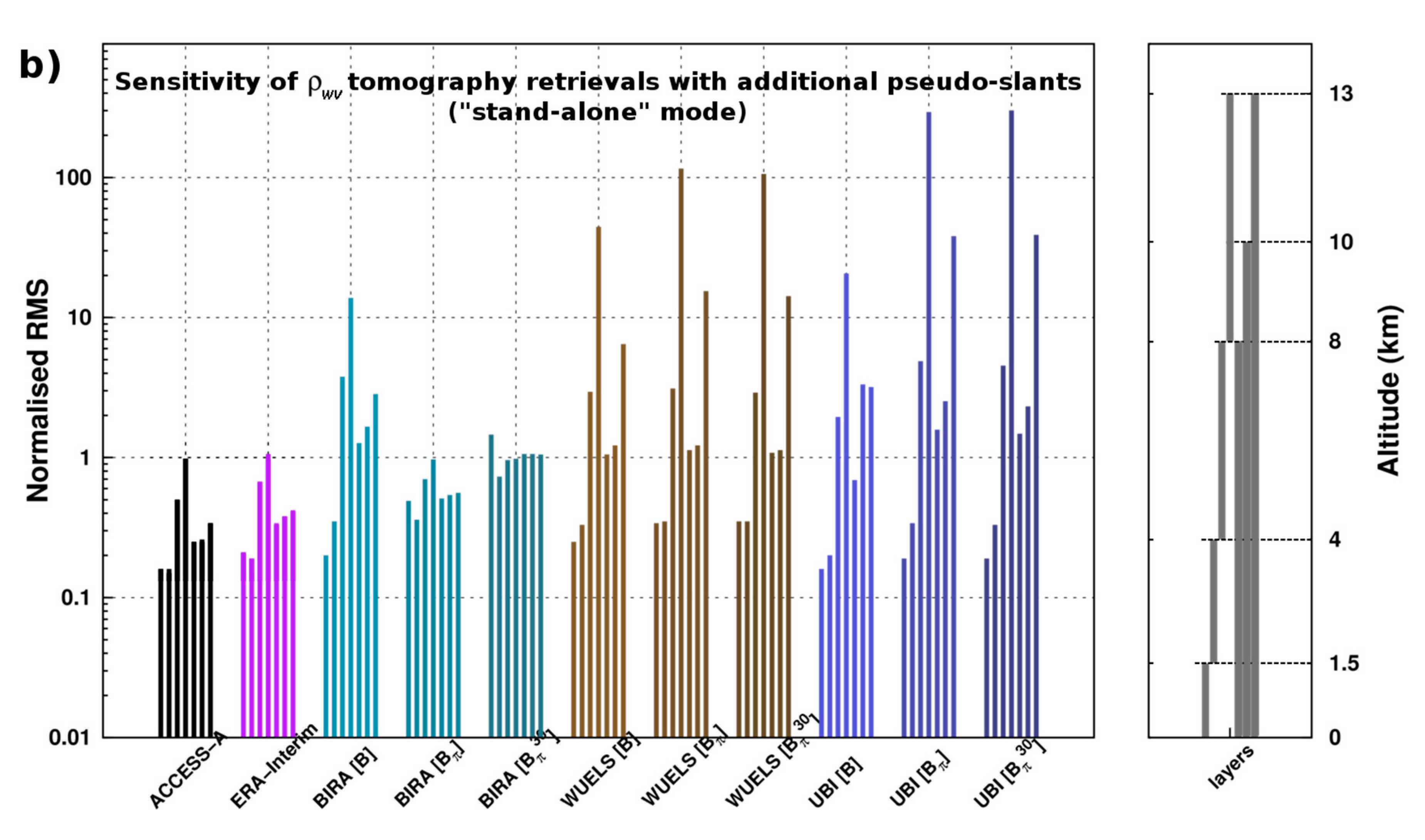
5.1.2. Use of Pseudo-Slant Observations

This section presents a methodology which is based on adding pseudo-slant observations to the systems of equations to be solved. The pseudo-slants were implemented according to the orientation of the delay gradient [57]. To obtain homogeneous repartition of sites (based on the CORS network), a distance of 20 km on both sides of a station in the direction defined by the GPS gradient was considered. This means that for two pseudo-sites, the wet delay and the water vapour content were propagated at a 20 km distance using the amplitude of the gradient, i.e., the additional wet delay equal to the multiplication of the gradient by the distance. The pseudo-SLANT_GPS in the direction of the GPS satellites was estimated using an isotropic mapping function (GMF in this case; see [37]) and considered in tomography calculations, as illustrated in Figure 5. Note also that two other pseudo-stations located at 10 km from the station were used, considering gradient orientation and its opposite direction. This makes for a total of four pseudo-sites with four sets of additional pseudo-slants (only two additional sets are illustrated in Figure 5).

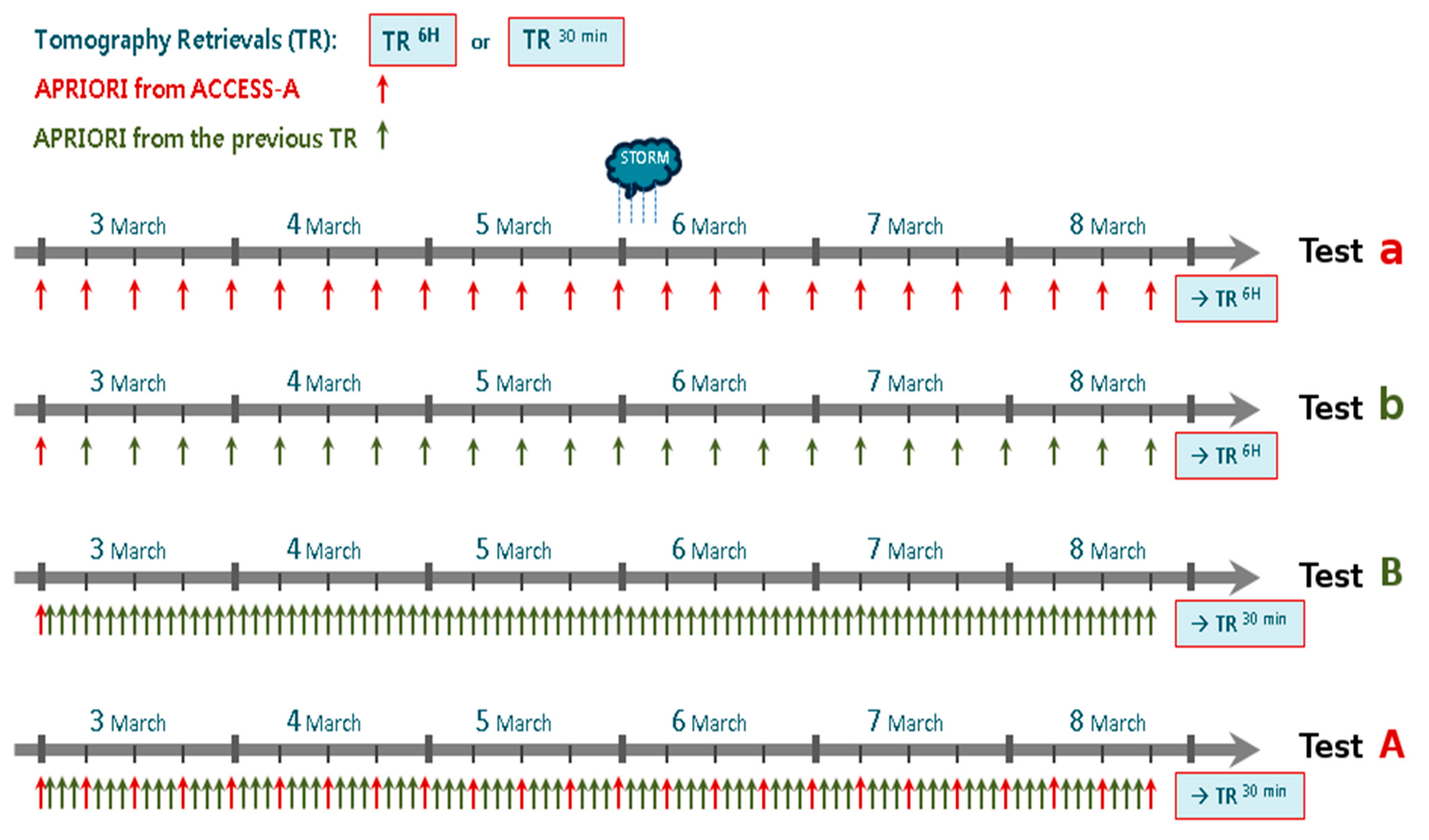
5.2. A Priori Condition and Improvement of the Convergence in the Inversion Process

This section investigates the ability to obtain an optimal stabilisation of solutions for five types of tomography software based on different techniques (singular value decomposition, damped least-squares adjustment, algebraic reconstruction technique, and Kalman filter). Four tests related to the a priori conditions used in calculations were studied to determine the best strategy. These four configurations were designed to test convergence in tomography calculations according to the a priori condition and time resolution of the tomography models (capital letters when the interval calculation was 30 min, i.e., tests A or B; lowercase letters when it was 6 h, i.e., tests a or b). An illustration of the configuration of these four tests is presented in Figure 6, in which arrows in red indicate when the a priori condition from ACCESS-A was considered in tomography calculations, and arrows in green indicate when this was the previous tomography retrieval (TR).

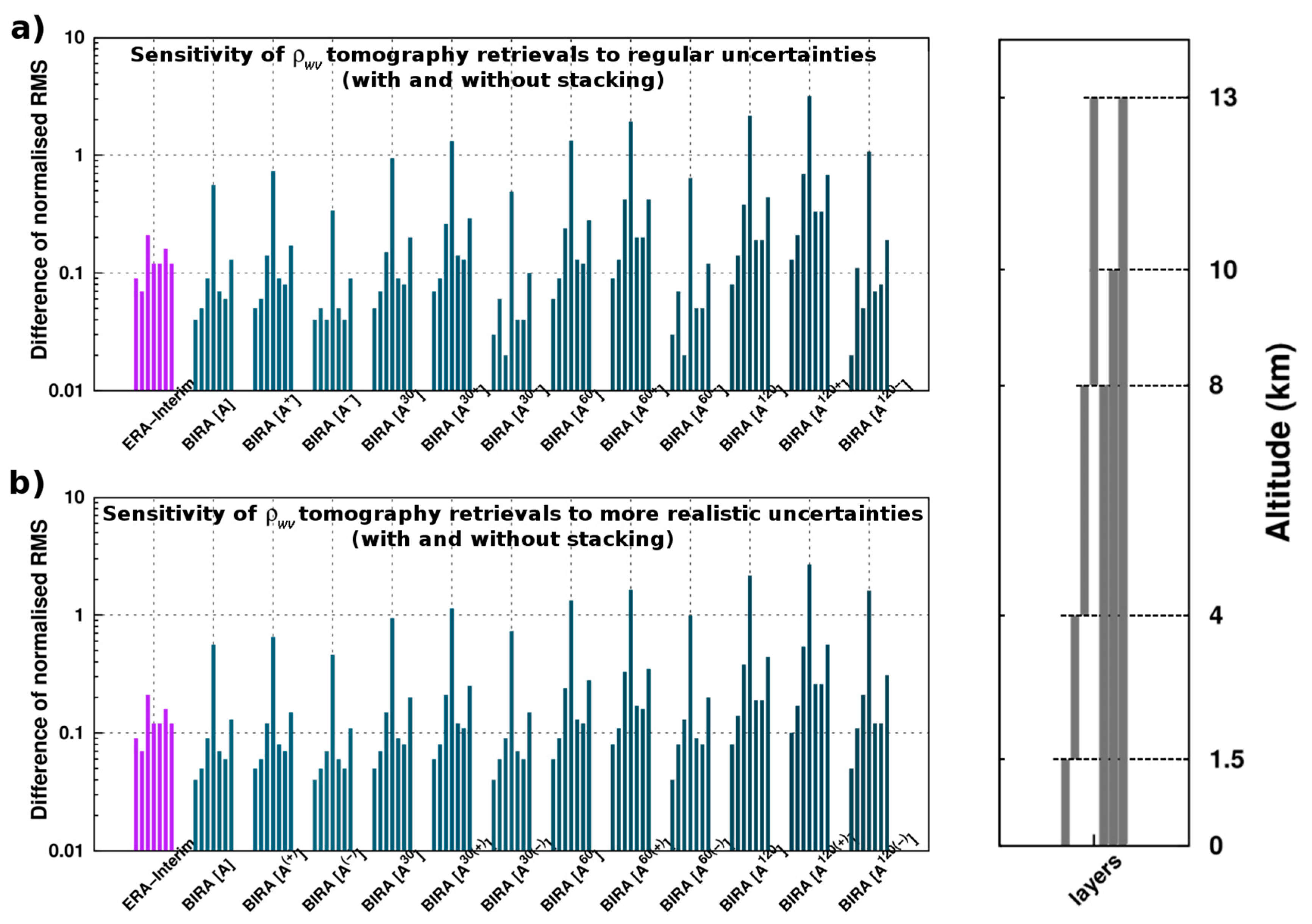
5.3. Sensitivity Tests Based on the Uncertainty of Slant Observations

The quality of slant observations is critical for obtaining optimal GNSS tomography retrievals. The strategy of this section was to modify slant observations using minimal/maximal uncertainties and to look at the impact on the quality of retrievals. The uncertainties of parameters acting for obtaining SWDs and SIWVs are presented in

Table 3. Absolute uncertainty and relative error of parameters related to GPS tomography. Legend: R_d, specific molar gas constant for dry air; R_w, specific molar gas constant for water vapour; k₁, k₂, k₃, k’₂, refractivity coefficients; P_S, surface pressure; T_m, mean temperature of the atmospheric column; g_m, gravity in the centre of the atmospheric column; ZTD, zenith total delays; ZHD, zenith hydrostatic delay; ZWD, zenith wet delay; κ, conversion factor; IWV, integrated water vapour content; SWD, slant wet delay; SIWV, slant-IWV; ${\mathrm{L}}_{\mathrm{sym}}^{\mathrm{wet}}$, isotropic wet component of SWD; ${\mathrm{L}}_{\mathrm{az}}^{\mathrm{wet}}$, anisotropic wet component of SWD; G_EW, East-West component of delay gradients; G_NS, North-South component of delay gradients.

Parameter	Value	Unit	Absolute Uncertainty	Relative Error
Rd	287.0586	J/(kmol K)	±0.0055	±0.002%
Rw	461.525	J/(kmol K)	±0.013	±0.003%
k1	77.60	K/hPa	±0.05	±0.064%
k2	70.4	K/hPa	±2.2	±3.125%
k3	373900	K2/hPa	±1200	±0.321%
k2’	22.1345	K/hPa	±2.2352	±10.090%
Parameter	Typical Value	Unit	Absolute Uncertainty	Relative Error
PS	1000	hPa	±2 (±1)	±0.200% (±0.100%)
Tm	285	K	± 1 (±0.5)	±0.351% (±0.175%)
gm	9.807	m.s−2	±0.022	±0.227%
ZTD	2.54	m	± Formal error + 0.010 (+ 0.005)	±0.497% (±0.296%)
ZHD	2.29	m	±0.011 (±0.007)	±0.494% (±0.326%)
ZWD	0.25	m	±0.019 (±0.010)	±8.605% (±4.503%)
κ	159	kg/m3	±1.335 (±1.053)	±0.840% (±0.622%)
IWV	40	kg/m2	±3.375 (±2.513)	±8.440% (±6.260%)
$L_{sym}^{wet}$	Variable *, mean: 0.765	m	Variable *, mean: ±0.069	Mean: ±9.020%
$L_{az}^{wet}$ and (GEW, GNS)	Variable *, mean: 0.027 [GEW, GNS] = [5, 5]	m (mm, mm)	Variable *, mean: ±0.003 (±0.001) ± Formal error + [0.8, 0.6] ([0.4, 0.2])	Mean: ±10.249% (±5.137%)
SWD	Variable *, mean: 0.792	m	Variable *, mean: ±0.072 (±0.039)	Mean: ±9.091% (±4.924%)
SIWV	Variable *, mean: 122	kg/m2	Variable *, mean: ±12.230 (±6.238)	Mean: ±10.003% (±5.098%)

* depends on the elevation of GPS satellite and data considered.

. These parameters are the specific molar gas constant for dry air (R_d), the specific molar gas constant for water vapour (R_w), the refractivity coefficients (k₁, k₂, k₃, and k₂’ = k₂ − k₁.R_d/R_w), the surface pressure (P_S), the mean temperature of the column of air (T_m), the gravity in the centre of the atmospheric column pressure (g_m), the GPS observation of ZTD, and estimations of ZHD, ZWD, factor κ, and IWV. More details regarding the links of these physical parameters with ZWD and IWV (based on preliminary results from [34,50,58]) and the impact of their uncertainties on simulations (using a high-resolution non-hydrostatic model during severe weather situations) are presented in Brenot et al. [40]. Finally, two kinds of empirical mapping functions (NMF of Niell [59] and GMF of Böhm et al. [37]) have been considered to estimate the impact on SLANT_GPS and retrievals from GPS tomography. The impact on the precision of slant retrievals is presented by an absolute uncertainty (in the unit of the tested parameter) and by a relative error (in %). In the upper six lines of Table 3 it can be seen that the parameter with the highest relative error is the refractivity coefficient k’₂. The uncertainties of refractivity coefficients (k₁, k₂, k₃) provided by Bevis et al. [60] were used, and the combination of higher and lower values for these coefficients show an absolute error of about 10% for k’₂.

The bottom part of Table 3 presents absolute uncertainty and relative error for typical values of the estimated parameters. In these columns, two types of uncertainty were considered: one which was more conservative (the higher values) and one which was more realistic (the lower values). The results related to the more realistic absolute uncertainty and relative error are presented in brackets (e.g., a conservative uncertainty of P_S of 2 hPa against a more realistic uncertainty of 1 hPa). To estimate the uncertainty of g_m, the bias between the formulation of Saastamoinen [39] and the formulation of Vedel et al. [61] was considered (a relative error of about 0.2%). The relative error in ZTD measurements and in P_S, T_m, and ZHD estimates are low (<0.5%). On the other hand, the relative errors of ZWD and IWV are high, being about 8.5% for both for the conservative error and 4.5% and 6.2%, respectively, for the more realistic error. The analytic expression of the conversion factor κ takes into account k₃, k’₂, and R_d coefficients and T_m parameters [34]. T_m was estimated using output from the ACCESS-A model with an absolute uncertainty of 1 K (or 0.5 K). A moderate relative error was found for κ (<1%). Note that this parameter was able to obtain a higher relative error in the case of severe weather conditions and the occurrence of hydrometeors in the path travel of the GNSS signal [40]. The last parameter that considered was the uncertainty of the mapping function. The uncertainty of SLANT_GPS was estimated using a satellite visible from one station during one epoch of measurements (10 satellites).

To test the uncertainty of SWDs, the uncertainty of ${\mathrm{L}}_{\mathrm{sym}}^{\mathrm{wet}}$ of Equation (2) was considered using the absolute error of the NMF and GMF mapping function [37,59], as shown in Equation (12)

$${\mathrm{L}}_{\mathrm{sym}}^{\mathrm{wet},\mathrm{MIN}}(є)=\mathrm{ZWD}·\left(\mathrm{GMF}-\left|\mathrm{NMF}-\mathrm{GMF}\right|\right)$$

(12)

$${\mathrm{L}}_{\mathrm{sym}}^{\mathrm{wet},\mathrm{MAX}}(є)=\mathrm{ZWD}·\left(\mathrm{GMF}+\left|\mathrm{NMF}-\mathrm{GMF}\right|\right)$$

(13)

where GMF = ${\mathrm{mf}}_{\mathrm{sym}}^{\mathrm{wet},\mathrm{GMF}}(є)$ and NMF = ${\mathrm{mf}}_{\mathrm{sym}}^{\mathrm{wet},\mathrm{NMF}}(є)$. This shows a relative error of 9%. To obtain the uncertainty of ${\mathrm{L}}_{\mathrm{az}}^{\mathrm{wet}}$ of Equation (3), the formal error of gradients provided by geodetic software and the error estimated by [17] were considered. This brought about a relative error of 10% (or 5%, to be more realistic). Finally, the uncertainties of SWD and SIWV were found to be, respectively, 9% and 10%, with more realistic errors of 5% occurring for both.

6. Results of Methodological Improvement in GPS Tomography

Three GPS tomography methodologies were investigated and combined. The improvement of geometrical representativeness is linked to convergence in tomography calculations. Independently, a sensitivity test of the perturbation of the quality of slant observations, inputs of GNSS tomography, has been presented and was combined with the two others improvements to investigate the interest in this approach in meteorological applications. The first methodological improvement targets a better geometrical distribution. The second concerns a better convergence behaviour in tomography solutions with respect to the a priori condition applied and the time resolution of calculations (i.e., tests a, b, B, A in

Table 4. Tests studied divided by data type, a priori data configuration, and stacking settings.

Data Type	Initial Observations (IO)		IO with Additional Pseudo-Observations		Observations Modified Considering Uncertainties
					Positive	Negative	Positive	Negative
	Every 6 h	First Epoch Only	Every 6 h	First Epoch Only	Every 6 h		First Epoch Only
No	Tests a and A	Tests b and B	Test Aπ	Test Bπ	Tests A+, A(+)	Tests A−, A(−)	Tests B+, B(+)	Tests B−, B(−)
30 min	Test A30	Test B30	Test Aπ30	Test Bπ30	Tests A30+, A30(+)	Tests A30-, A30(−)	Tests B30+, B30(+)	Tests B30-, B30(−)
60 min	Test A60	Test B60	-	-	Tests A30+, A30(+)	Tests A30-, A30(−)	Tests B30+, B30(+)	Tests B30-, B30(−)
120 min	Test A120	Test B120	-	-	Tests A120+, A120(+)	Tests A120-, A120(−)	Tests B120+, B120(+)	Tests B120-, B120(−)

, as illustrated in Figure 6). The configurations of tests A and B were used as references and the improvement of the geometrical distribution was investigated using stacking data (e.g., tests A³⁰, A⁶⁰, and A¹²⁰) and/or pseudo-slant observations (e.g., tests A_π and A_π³⁰). In addition, via a third way of testing and again using the configurations of tests A and B as references, the impact of the observational uncertainty on the quality of tomographic results was studied (e.g., tests A⁺ and A⁻). Table 4 shows an overview of all tested model settings.

For all the tests presented in Table 4, spatial and temporal distributions of the $N_w\mathrm{or}{\rho }_{wv}$ parameters were determined for three types of data (“initial observations (IO)”, “IO with additional pseudo-observations”, and “observations modified considering uncertainties”). The interval calculation for all the tests in Table 4 was found to be 30 min (except for tests a and b). Using the configuration of test A or B, other tests with 30, 60, and 120 in the superscript (i.e., A³⁰, A⁶⁰, and A¹²⁰) were meant to test improvement of stacked data on solutions using 30, 60, and 120 min -stacked data, respectively. Tests with π in the subscript (i.e., tests A_π and B_π) were set up to test the improvement of using pseudo-slants solutions and were combined with the test of stacked data (i.e., A_π³⁰, A_π⁶⁰, and A_π¹²⁰). The impact of the uncertainty on solutions (columns “positive” and “negative” of Table 4) was investigated for two types of uncertainty: regular, with labels “+” and “-”, and more realistic, with labels “(+)” and “(−)”. The “positive” column indicates uncertainty increasing slant observations (superscript ⁺ or ⁽⁺⁾ used in the name of the test, e.g., test A⁺ or A⁽⁺⁾) and the “negative” column indicates uncertainty decreasing slant observations (superscript ^– or ⁽⁻⁾, e.g., test A⁻ or A⁽⁻⁾). The impact of uncertainty on solutions was combined with the test of stacked data (i.e., A³⁰⁽⁺⁾, A⁶⁰⁽⁺⁾, and A¹²⁰⁽⁺⁾).

To visualise the results and validate our methodological improvements, tomography retrievals were compared with external observations (profiles of $N_w\mathrm{and}{\rho }_{wv}$ from RS and RO). Profiles of $N_w\mathrm{and}{\rho }_{wv}$ from ACCESS-A were also considered (as an example of forecasts) and were the a priori conditions used in our tomography calculations. ERA-Interim [62] profiles were also prepared and compared.

Three various comparisons are shown within this study: GPS tomography versus RS profiles, GPS tomography versus RO profiles, and individual GPS tomography solutions versus each other or ACCESS-A and ERA-Interim fields. Since all mentioned techniques sense tropospheric water vapour in a different way, the presented comparisons were based on different approaches. To compare RS profiles with GPS tomography results, or with ACCESS-A and ERA-Interim fields, RS profiles were linearly interpolated to individual heights of the tomography grid. Tomography retrievals and ACCESS-A/ERA-Interim estimates were then bilinearly interpolated to positions of RS stations; RS profiles were assumed to be vertical (wind field was not considered, given the assumption that tomography outputs and RS profiles are simultaneous). Slant RO profiles were derived at heights of the tomography grid. Then, tomography retrievals and ACCESS-A/ERA-Interim estimates were bilinearly interpolated to latitudes/longitudes of RO profiles. For comparisons between two individual GPS tomography solutions or between a GPS tomography solution and ACCESS-A/ERA-Interim fields, no interpolation had to be applied and a direct confrontation in 3D tomographic voxels was realised (for ACCESS-A/ERA-Interim the closest grid points to the tomography grid were considered).

6.1. Results Regarding the Improvement of Geometrical Distribution

An increased geometrical distribution can be a way to obtain a better stabilisation of tomography solutions. More voxels being crossed by slant GPS observations (SLANT_GPS) can improve the understanding of this meteorological situation. However, this means that more inputs are considered in tomography processing.

Table 5. Geometrical distribution and time processing of our sensitivity tests. Legend: SLANT_GPS, slant GPS observations and pseudo-observations.

Type of Tomography Calculation		No Stacking	Stacked Data (30 min)	Stacked Data (60 min)	Stacked Data (120 min)	Pseudo-Slant Observations
						No Stacking	Stacked Data (30 min)
Mean Number of SLANTGPS		685	1370	2050	3400	3140	6275
Geometrical Distribution (% of Voxels Crossed) for Different Layers	0–1 km	51.2	51.2	51.2	51.4	82.9	84.6
	1–2 km	58.3	58.3	58.3	61.6	88.0	89.4
	2–4 km	65.6	66.0	67.4	72.2	93.1	93.1
	4–6 km	73.6	75.0	76.4	82.6	95.8	97.2
	6–9 km	77.0	81.3	84.0	87.5	92.4	93.1
	9–13 km	61.8	67.4	67.8	70.6	64.6	68.0
	All	67.8	69.3	69.5	72.0	92.8	93.7
Indicator of Mean Time of Processing (minutes)		0.5	1	2	8	7	130

shows the status of the geometrical distribution (% of voxels crossed by SLANT_GPS for the different tests considered) inside the inner tomography grid. The mean number of SLANT_GPS is provided for each epoch of calculation. Note that the mean time of processing is also indicated (a 2.66 GHz processor with 24 GB RAM was used) as being a key parameter for nowcasting (non-linear quasi-quadratic dependency with the number of inputs). According to the distribution of rays from GPS stations inside the tomographic grid, for the 288 times of measurements from 3 to 10 March, 2010, the mean percentage of voxels retrieved by our classic tomography models was 67.8% for the whole tomographic grid (geometrical distribution obtained without stacking and pseudo-slant observations). Using stacked slant data (30, 60, or 120 min stacking), an increase in the geometrical distribution (+1.5%, +1.7% or +4.2%, respectively) and a consequent increase in the time of processing (×2, ×4, or ×16, respectively) was observed. Note that in these cases of stacked data, slants were only considered every 30 min, not continuously (this was not relevant for our tomography grid, which had a horizontal resolution of 50 km). The layers between 2 and 9 km show the main results with a high increase of geometrical distribution (about +10%). Using pseudo-slant observations, an increase of +25% can be observed for all layers on average, with an increase of +30% for the layers between 0 and 4 km and an increase of +20% for those between 4 and 9 km. The geometrical distribution only increased by +3% for the top layer of between 9 and 15 km (for more details regarding pseudo-slants, see Section 5.1.2).

6.1.1. Interest in Data Stacking for Mid-Troposphere Retrievals

Three sets of stacked slant data were tested, namely, 30, 60, and 120 min stacking. Hence, the two processing strategies illustrated in Figure 6 by tests A and B were applied for tests (A³⁰, A⁶⁰, A¹²⁰) and (B³⁰, B⁶⁰, B¹²⁰), respectively.

In Figure 7a, the results for tests (A³⁰, A⁶⁰, A¹²⁰) are compared to test A, as this solution was also initiated with a priori data every 6 h. The three sets of solutions for the three models show different patterns. We can see that the 8–13 km layer was not well solved by the tomography models, which consequently impacted the overall result (respectively, lines/layers 4 and 7). Looking at the layers under 10 km, the Wroclaw University of Environmental and Life Sciences (WUELS) and University of Beira Interior (UBI) models show a similar performance for tests A and A³⁰ (shortest 30 min stacking) and an improved accuracy for the longer stacking period. WUELS reached a better performance in test A⁶⁰, i.e., for 60 min stacking, with a normalised root mean square (RMS) of 0.52 g/m³ compared with 0.96 g/m³ for test A. Both UBI and the Royal Belgian Institute for Space Aeronomy (BIRA) model obtained comparable accuracy retrievals in the first two layers to ACCESS-A values and retrievals which were slightly better than ERA-Interim (normalised RMS of 0.16 g/m³ versus 0.21 g/m³). Note that normalised RMS values were computed from relative differences of two corresponding values from two solutions. The relative difference means that an absolute difference of two values is divided by one of the values. This method of statistics computation allows a reasonable comparison of studied ${\mathrm{N}}_{\mathrm{w}}{\mathrm{and}\mathsf{\rho }}_{\mathrm{wv}}$ parameters, whose absolute values change significantly with height.

The results shown in Figure 7b for tests (B³⁰, B⁶⁰, B¹²⁰) were compared to test B, as this solution was also initiated with a priori data from NWP (i.e., ACCESS-A) only in the first epoch, the so-called “stand-alone” mode. The WUELS and UBI models in tests (B³⁰, B⁶⁰, B¹²⁰) performed very similarly to test B as long as the troposphere below 4 km is considered; in the 4–8 km layer, both delivered improved solutions: WUELS showed in test B⁶⁰ a 30% improvement over test B and UBI performed in test B³⁰ about 20% better than in test B. However, both solutions were worse than ACCESS-A and ERA-Interim, especially above 8 km. The BIRA model produced somewhat different results: in the 0–1.5 km layer the solution for test B³⁰ was better than that in test B and in ERA-Interim (with a normalised RMS of 0.19 g/m³ versus 0.20 g/m³ and 0.21 g/m³, respectively). In all higher layers until 13 km test B¹²⁰ was much better than test B, while for the top-most layer it attained a better performance than ACCESS-A and ERA-Interim (0.90 g/m³ versus 0.98 g/m³ and 1.06 g/m³, respectively). Whatever the tomography model used, the performance in the 0–8 km layer was better in test (B³⁰, B⁶⁰, B¹²⁰) than in test B; however, above an 8 km height, the best performance was found (in the BIRA and WUELS models) for the longest stacking period of 120 min (test B¹²⁰). Note that for BIRA, test B¹²⁰ showed even better results than ACCESS-A (1.06 g/m³ versus 0.90 g/m³).

6.1.2. Interest in Pseudo-Slant Observations for Low- and Mid-Troposphere Retrievals

This section investigates the interest in adding pseudo-slants observations (SLANT_GPS) in tomography retrievals. As shown in Table 3, the use of pseudo-slants increased the geometrical distribution by +30% and +20% for the 0–4 km and 4–9 km layers, respectively. To test the implication of improving the geometry with pseudo-slant observations, test A (with a regular initialisation from NWP outputs; see Figure 6) and test B (only previous tomography retrievals used as a priori, making a ‘stand-alone solution’) were compared with tests A_π and B_π, respectively (tests that considered pseudo-observations); see Figure 8.

Tests A_π³⁰ and B_π³⁰ (with 30 min data stacking) are also shown. Tests with 60 and 120 min stacked pseudo-slants, as originally planned, were not processed because they are not relevant for nowcasting (they have time windows which are too long and involve a significant increase of time processing of about ×250 and ×4000, respectively). The comportments of the three models considered were different. While WUELS improved in tests A_π and A_π³⁰ over test A (an improvement of about 15%), a degradation was able to be observed in tests B_π and B_π³⁰ over test B (the normalised RMS was multiplied by 2.4 g/m³ and 2.2 g/m³, respectively). This conclusion was mainly driven by analysis of the 8–13 km layer. Even with an improvement, the results were still far from the RS data, which had a normalised RMS of about 73 g/m³ for WUELS and about 1 g/m³ for ACCESS-A and ERA-Interim. For the UBI model, the same tropospheric layer drove the result, but with a degradation according to both tests A and B (the normalised RMS was multiplied by 6 and 12, respectively). For the BIRA model, tomography retrievals using pseudo-SLANT_GPS with a regular initialisation from NWP showed a small degradation from a normalised RMS of 0.43 g/m³ to 0.87 g/m³ and 1.27 g/m³ for tests A_π and A_π³⁰, respectively (this was mainly driven by the high troposphere layer). However, the use of pseudo-SLANT_GPS with ‘stand-alone initialisation’ (giving an overall normalised RMS of 2.84 g/m³ for test B) obtained a consequent improvement with an overall RMS of 0.56 g/m³ and 1.05 g/m³ for tests B_π and B_π³⁰, respectively. The improvement took place in five of the seven layers (altitude ranges) studied; no improvement was observed in the 0–1.5 km and 1.5–4 km layers. In the 8–13 km later, the BIRA model even showed a slightly better performance than ACCESS-A (which had a normalised RMS of 0.97 g/m³ for BIRA compared with 0.98 g/m³ for ACCESS-A).

The recommendation of improving the geometrical matrix of tomography retrievals with pseudo-slant observations was applied using data from the Belgian dense network (baselines from 5 to 30 km) during the pouring rains of 15–17 August, 2010 (a weather depression called Yvette by German meteorologists). GAMIT software was used to calculate ZTDs and gradients with a respective time resolution of 15 and 30 min (see Brenot et al. [40] for more details regarding the settings of these measurements). SIWVs were obtained using the GMF mapping function and ground pressures and temperatures from synoptic stations (no post-fit residuals were considered). The horizontal resolution of the tomography grid was 10 × 10 km and a vertical resolution of 500 m (for up to 10 km) was set. Figure 9 presents a comparison of profiles from tomography retrievals and ALARO NWP outputs with RS data from the Uccle station (Brussels) at 12:00 UTC on 16 August, 2010. The a priori condition from the ALARO NWP model (4 km resolution) was considered and applied to retrieve water vapour density from GPS tomography (employing the classical method and using pseudo-SIWVs).

The normalised RMS between RS and a priori ALARO, RS and tomography (classical), and RS and tomography (pseudo-slants) were 1.00 g/m³, 0.97 g/m³, and 0.89 g/m³, respectively, for all layers. These normalised RMS values became 0.47 g/m³, 0.44 g/m³, and 0.39 g/m³ in the 0–6 km layer and 0.11 g/m³, 0.09 g/m³, and 0.02 g/m³ in the 0–3 km layer. This confirms interest in using pseudo-slant observations in GPS tomography.

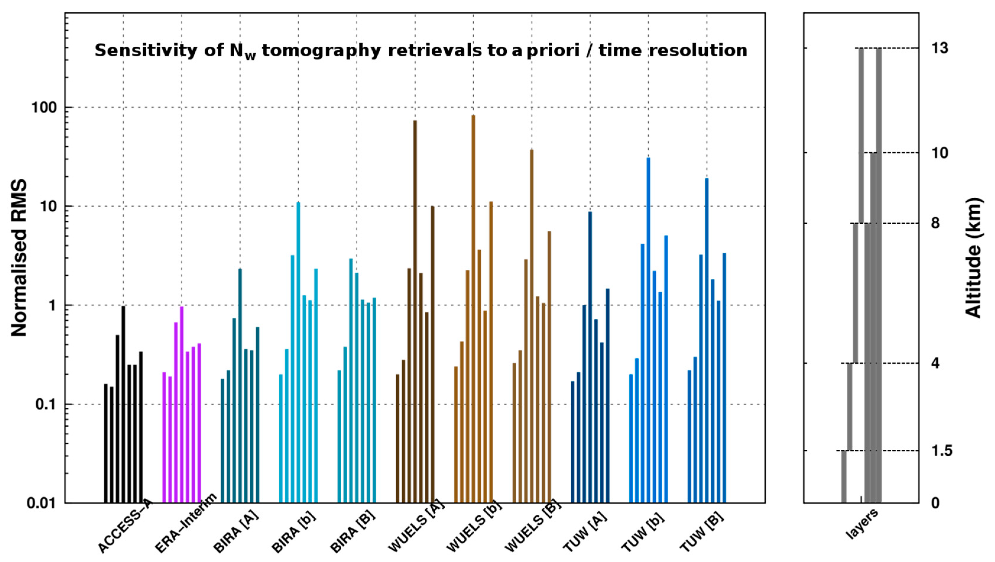
6.2. Convergence of Tomography Solutions with Respect to A Priori Conditions and Time Resolution of Processes

To look at the impact of a priori conditions on tomography retrievals (for 3–8 March 2010), this section focuses on tests A, b, and B, as presented in Figure 6. RS were launched at 00:00 and 12:00 UTC, so the results of tests A and a were the same.

Figure 10 shows that in test A, wet refractivity estimates from GPS tomography models were usually the best in the bottom part of the troposphere (below 1.5 km), with two out of three models displaying a comparable performance (less than 10% degradation) to ACCESS-A, namely, BIRA and TUW. Tomography retrievals (test A for BIRA, WUELS, and TUW) in the bottom part of the model showed better agreement with RS than ERA-Interim results, and TUO displayed a similar performance (not shown in Figure 10). However, this shows that this positive impact of GPS observations on the estimated troposphere state was diminished once the a priori data introduced to the tomography model were no longer fed in every epoch (test b) or the time resolution of estimates became higher (i.e., 30 min for test B). In the second investigated layer (1.5–4 km) the tomography-retrieved refractivity displayed usually the same or slightly worse accuracy than the NWP-based solutions: BIRA and TUW displayed 0.02 ppm (test A). Once the a priori data were not fed into the solution, the quality of retrievals dropped substantially, by almost 40%. The retrievals in the higher layers, namely, 4–8 km and 8–13 km, for all models in this study, were substantially worse than the ACCESS-A retrieval in all three tests. It also should be noted that the TUO retrieval, even though less accurate than ACCESS-A, provided better solutions than ERA-Interim for all 10 km, producing a normalised RMS of 0.36 and 0.38.

A similar pattern was obtained for models producing water vapour density (not presented). Compared to radiosonde in Melbourne, the tomography solution (test A) was of similar quality to the ACCESS-A model in the first two layers of the atmosphere (below 4 km), especially for the models BIRA and UBI, while WUELS and TUO showed a slightly lower performance. Between 4–8 km, only BIRA and TUO retrievals were of useful accuracy, while WUELS and UBI showed five and four times lower performance, respectively. Interestingly, the 8–13 km retrieval from TUO showed a better performance than ACCESS-A data (displaying a normalised RMS of 0.94 g/m³ and 0.98 g/m³). Test b and B showed a much worse solution, especially in the higher levels of the model. The BIRA model in test A reached a better agreement with RS than ERA-Interim results across the whole 0–10 km profile (producing a normalised RMS of 0.28 g/m³ and 0.38 g/m³).

6.3. Results Regarding the Impact on the Precision of Slant Retrievals

To investigate the impact on the precision of slant retrievals, the uncertainties of parameters acting for obtaining SWDs and SIWVs were considered; see Section 5.3. The higher and lower estimates of slants (as shown in Table 3) were used to look at the repercussions on tomography solutions. Figure 11 highlights differences of normalised RMS (related to ${\rho }_{wv}$ observations) from 13 datasets (compared to RS, e.g., RS–BIRA [A³⁰⁺]) with RS–ACCESS-A. A highlight of eight tests regarding the impact of uncertainty is presented (tests A⁺ and A⁻, for higher and lower slants, respectively, without stacking; tests A³⁰⁺ and A^30- with 30 min stacking; tests A⁶⁰⁺ and A^60- with 60 min stacking; and tests A¹²⁰⁺ and A^120- with 120 min stacking). Superscripted labels + and - and (+) and (−) refer to regular and more realistic uncertainties (see values in brackets in Table 3), respectively, shown in Figure 11a,b. These eight tests were used a priori from ACCESS-A every 6 h and can be compared to tests A, A³⁰, A⁶⁰, and A¹²⁰. The difference in normalised RMS from RS–ERA-Interim with RS–ACCESS-A is also presented. To avoid differences in normalised RMS which were less or equal to 0.01 g/m³ in the logarithm scale of the y-axis, an offset of +0.03 g/m³ was considered.

We found consistent comportment of tomography retrievals according to the type of uncertainty (regular with strong impact and more realistic with weak impact). We also observed that stacked data amplified the impact of uncertainty in tomography retrievals. Considering RS–ACCESS-A as a reference, the sensitivity of the bias (i.e., the difference of normalised RMS) between RS and tomography water vapour density for different kinds of slants (maximum/minimum uncertainty with regular/more realistic errors), in comparison to the RS–ERA-Interim, showed interesting results regarding the quality and possible improvements in SLANT_GPS as well as the validation of the NWP model using tomography retrievals. Adding an uncertainty measure to the observation matrix increased the accuracy of stochastic modelling for tomography retrievals and using a priori every 6h (in Figure 11) and stacked solutions (e.g., A³⁰⁽⁻⁾, A⁶⁰⁽⁻⁾, and A¹²⁰⁽⁻⁾) led to a better performance in the bottom 1.5 km. In the upper layer (1.5–4 km), these solutions were of lower quality than in ACCESS-A, but still better than those of ERA-Interim. The 4–8 km layer was again better resolved using the BIRA model in tests A³⁰⁽⁻⁾ and A⁶⁰⁽⁻⁾. The topmost layer was of lower quality in all tests. The same kinds of tests were performed using a priori from ACCESS-A only for the first epoch (to be compared with tests B, B³⁰, B⁶⁰, and B¹²⁰). In comparison to the results of Figure 11, the impact of the uncertainty was amplified due to the stand-alone situation of the tomography technique which was less constrained by the a priori condition and ACCESS-A model. To illustrate this, we looked at the 4–8 km layer and the comparison of ${\rho }_{wv}$ from RS with estimates from ACCESS-A, ERA-Interim, test A³⁰, test A³⁰⁺, and test A^30-. We found respective normalised RMS values of 0.50 g/m³, 0.67 g/m³, 0.61 g/m³, 0.72 g/m³ (0.67 g/m³ for test A³⁰⁽⁺⁾), and 0.48 g/m³ (0.55 g/m³ for test A³⁰⁽⁻⁾), and also looked at a comparison with test B³⁰, test B³⁰⁺, and test B^30-, which showed respective normalised RMS values of 3.49 g/m³, 3.50 g/m³ (3.17 g/m³ for test B³⁰⁽⁺⁾), and 2.11 g/m³ (2.49 g/m³ for test B³⁰⁽⁻⁾).

7. Cross-Comparison of Tomography Models with Profiles from External Observations

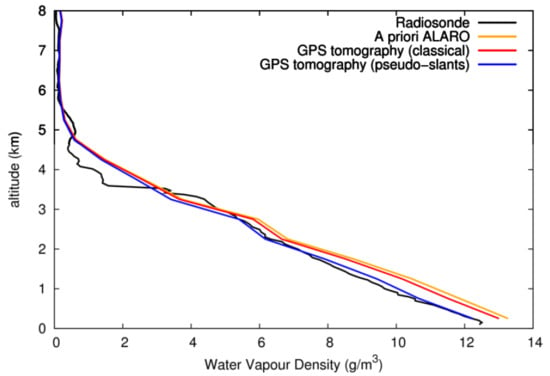
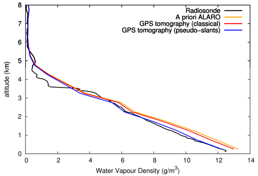
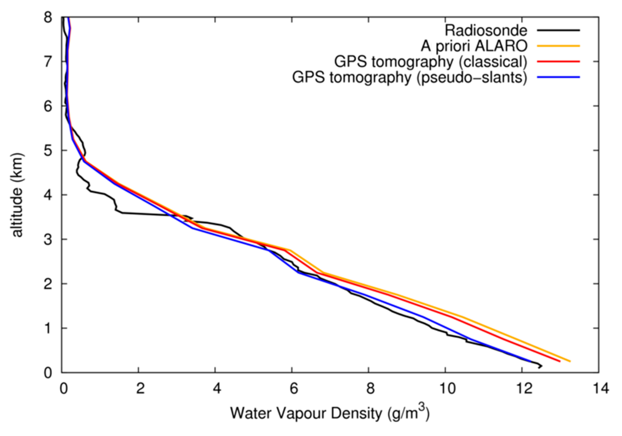
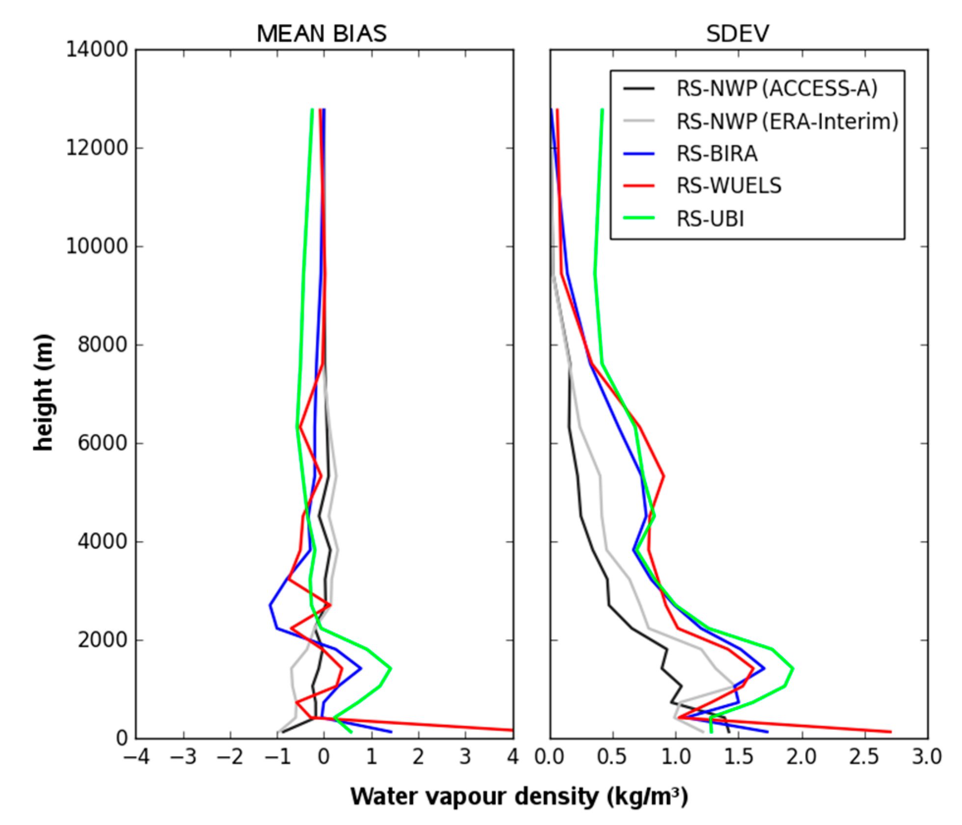
7.1. Comparison with Profiles from Radiosondes

Figure 12 illustrates the comportments of ${\mathsf{\rho }}_{\mathrm{wv}}$ retrievals from three tomography models (BIRA, UBI, and WUELS) with respect to Melbourne RS estimates during the whole five-day period; comportments of NWP (ACCESS-A or ERA-Interim) are also presented. Even ACCESS-A and ERA-Interim show ${\mathsf{\rho }}_{\mathrm{wv}}$ estimates closer to RS measurements than the tomography models, and it is possible to notice that the three tomography models show the same ${\mathsf{\rho }}_{\mathrm{wv}}$ pattern in the 0–4 km layer. A trend of moistening was observed in the low troposphere by GPS tomography and was not seen by RS and ACCESS-A NWP. Such features could be further studied by ensemble tomographic processing, which could be a way to identify anomalies in the low troposphere with respect to NWP or other measurement techniques. Note that tomography outputs and RS were assumed to be simultaneous (without considering the wind field that affected the trajectory of RS profiles). These assumptions could be the reason for the difference between tomography models and RS observations.

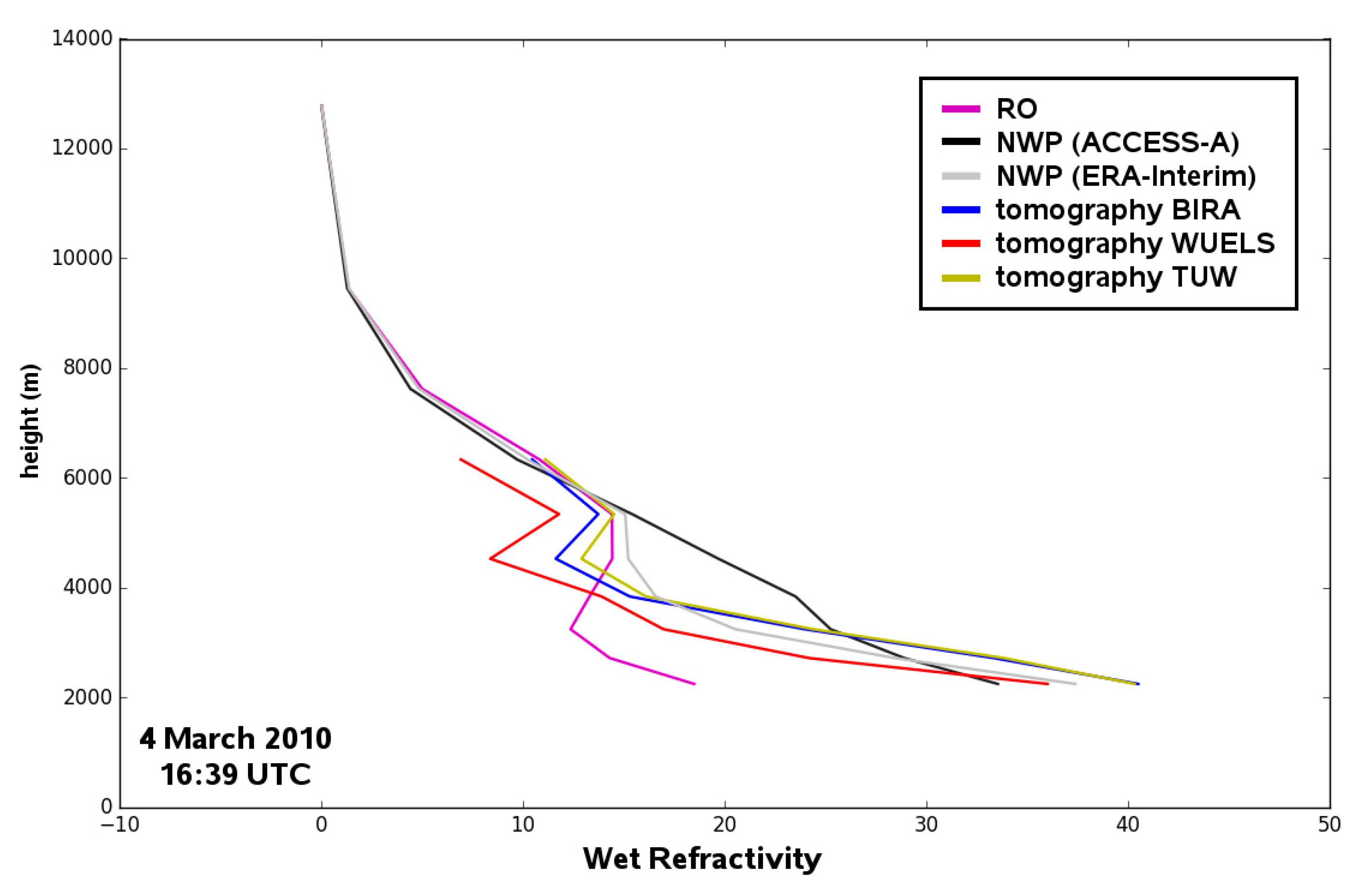
7.2. Comparison with Profiles from Radio-Occultations

From 3 to 8 March, 2010, there were four RO events reported by CDAAC that coincided with the location of our tomography network. The $N_w$ profiles from RO were compared with the BIRA, WUELS, and TUW model results, whereas the BIRA, WUELS, and UBI models were compared to the ${\rho }_{wv}$ profiles obtained from RO (the wetPrf product). The profiles collected on 3 March, 2010 08:07 UTC, 8 March, 2010 05:36 UTC, and 8 March, 2010 07:33 UTC (see Figure 1) showed no significant difference between RO (mean normalised bias from 10 to 20%), tomography retrievals, and ACCESS-A and ERA-Interim results, and followed a typical exponential pattern. Hence, these profiles will not be discussed further.

Figure 13 presents profiles which run from the south–west towards the north–east over the Australian Alps (see Figure 3) on 4 March, 2010 at 16:39 UTC (08:39 a.m. local time). Over 6 km the radio-occultation (RO) profiles are outside the inner tomography grid. For this reason, only RO and Numerical Weather Prediction (NWP) models show estimates of wet refractivity ($N_w$) over 6 km in Figure 13. The tomography solution for $N_w$ is the one referred to in Table 4 as “no stacking”, with a priori data fed into the model only in the first epoch. The results of the WUELS, BIRA, and TUW tomography models were similar, distinguishing one inversion layer at heights between 4 and 6 km (we can define this as a $N_w$ anomaly). For the RO profile, there were also local minima at these heights; however, the largest inversion occurred below 4 km. The RO- and tomography-based values of $N_w$ and ${\rho }_{wv}$ significantly differed from the ACCESS-A results in the lowest layer, as the latter did not show any inversion. The ERA-Interim result for this particular location was much closer to the tomography solution (BIRA and WUELS) and RO retrievals, showing a slight inversion between 5 and 6 km. The $N_w$ anomaly retrieved by both tomography models is a relevant piece of information for nowcasting.

7.3. Selected Results–Focus on Tomography Network in the East and during Selected Epochs

Based on the day of the previous investigated RO profile, we decided to verify the performance of the tomography models with respect to NWP forecasts in the eastern part of this model (orange/red pixels with high top cloud detected by GOME-2 in Figure 1a). The investigation was focused on the most accurate processing test A³⁰ and times 12:00 and 18:00 UTC on 4 March 2010 (see Figure 14).

First of all, we can see in Figure 14 that the BIRA and TUW models were in better agreement with ACCESS-A in the nine voxels (the south-eastern part of the network) than for all voxels, with the lowest discrepancy in the lower 10 km of the atmosphere being 0.15 ppm and 0.14 ppm, respectively, (for all the voxels, as shown in Figure 14a), and 0.10 ppm and 0.08 ppm, respectively, (for the nine voxels in the south-eastern part of the network, as shown in Figure 14b). At the same time, there was a much larger discrepancy between ACCESS-A and ERA-Interim in the same height range (0.23 for all the voxels and 0.29 for the nine voxels). Taking into account this disagreement, it should also be mentioned that the discrepancy between ERA-Interim and BIRA as well as ERA-Interim and TUW was smaller (about 0.18 ppm for all the voxels and 0.20 ppm for the nine voxels) in the height range 0–1.5 km than the respective discrepancies between ACCESS-A and ERA-Interim (0.27 ppm for all the voxels and 0.28 ppm for the nine voxels). For the 4–8 km layer, similar behaviour can be observed for model TUW (0.16 ppm for all voxels and 0.11 ppm for the nine voxels) versus ERA-Interim (0.20 ppm for both tests with nine or all voxels). The 1.5–4 km layer in the tomography models (BIRA and TUW) did not align well with ERA-Interim but aligned much better with the ACCESS-A solution (about 0.24 ppm versus 0.11 ppm for all voxels and 0.30 ppm versus 0.07 for nine ppm voxels). Note that ACCESS-A was better at modelling the 1.5–4 km layer in the region around Melbourne than ERA-Interim, and that a substantial improvement in the tomography model solution was most visible in this layer.

8. Summary, Conclusions, and Perspectives for Future Works

This study aimed to conduct sensitivity tests and methodological improvements by cross-comparing five independent tomography models. GPS data from the Australian CORS network were considered during a severe weather event, i.e., the 6–8 March superstorm of greater Melbourne. The same dataset of GPS slant observations was fed into tomography models and statistical results (bias, standard deviation, and root mean square error) have been shown in reference to independent observations from radiosonde and radio-occultation profiles. The inverse problem treated by GPS tomography was ill-posed due to non-homogenous distribution of slant observations through the 3D grid, but this was also ill-conditioned due to the high number of parameters physically embedded. This explains why the stabilisation of the tomographic solution remains a challenging task. In this study, software based on different techniques were considered to test improvements of the stabilisation of solutions. Three means of testing were investigated and combined: (1) the improvement of the geometrical representativeness of retrievals, (2) the influence of the a priori condition in the convergence process, and (3) the use of the uncertainty of inputs on tomographic solutions. This study has tested a number of variants for which the impact on the quality of tomographic results has been assessed. These variants are, notably, the interest in stacking data and the use of pseudo-slant observations, the a priori condition considered in the tomography process, and the quality of initial observations and the impact of observation uncertainty. We used five tomographic models, namely, BIRA, WUELS, TUO, UBI, and TUW (see the Appendices for more details about these models); the processed results were compared to data obtained from ACCESS-A and ERA-Interim outputs, RS profiles, and RO products.

Tomography models produce parameters that are usually of similar or worse quality than ACCESS-A retrievals (see Figure 7, Figure 8, Figure 10, Figure 11 and Figure 14) with few exceptions, i.e., in the bottom part of the troposphere for the BIRA and TUW tomography models (0–1.5 km), wet refractivity retrievals were of 0.5% better quality compared to ACCESS-A for tomography models fed with 6 h a priori data. Time stacking improved the solution with respect to non-stacking in all investigated cases without a continuous feed of a priori data (i.e., in tests B³⁰, B⁶⁰, and B¹²⁰). In addition, a short stacking period of 30 min (test B³⁰) gave a better response in the BIRA, WUELS, and UBI models (with 5, 3, and 17% respective improvements in the 0–8 km layer in comparison to test B), while for all other layers longer stacking worked better (120 min, test B¹²⁰): the lowest discrepancy between the tomography model and RS was found in the 8–13 km layer and the stacking test B¹²⁰, which showed an 8% improvement in the BIRA solution in comparison to ACCESS-A. The use of pseudo-slant observations showed variable results. Sometimes it did not bring about any visible improvement in terms of RMS, but in some cases (e.g., in the 0–10 km layer), the use of a pseudo-SLANT_GPS with ‘stand-alone initialisation’ obtained a consequent improvement (see tests B_π and B_π³⁰ in comparison to test B in Figure 8b; 0.56 g/m³ and 1.05 g/m³ were obtained, respectively, in comparison to 2.84 g/m³, for all the layers). The BIRA solution of test B_π³⁰ was indeed 1% better than that of ACCESS-A for the 8–13 km layer. Our sensitivity tests showed that when using 30 min stacking data, an improvement was obtained relative to RS profiles (a 5% improvement in the 0–1.5 km layer was observed for the BIRA model and an 18% improvement in the 4–8 km layer was observed for the UBI model) without bringing too old data into the tomography process, allowing for a proper understanding of the meteorological situation. However, the increase in the geometrical distribution (Table 3) was weak using only 30 min stacking data (+1.5 %). We found that the use of pseudo-slants can significantly improve the geometrical matrix of tomography retrievals (i.e., by +25 %, showing a better special representativeness) and can bring about, in some cases, an improvement (a five times lower RMS value was obtained for all the layers when comparing test B_π with test B for the BIRA model). The a priori condition tests on tomography show that the best results (with respect to RS) can be obtained using the best a priori. This is why, assuming that the ACCESS-A a priori was reasonably good (and close to the RS profiles), tomography retrievals, using regular a priori from NWP, obtain the best results (a three times lower RMS value was obtained for the 0–8 km layer, considering solutions from the BIRA, WUELS, and UBI models), illustrating that the “stand-alone” strategy (using the previous tomography retrievals as the a priori of the next calculation) is not always successful. A divergence in results is obtained, especially when the a priori is far from the real state of the atmosphere.

Figure 15 summarises the results of water vapour density retrievals obtained for three types of a priori conditions (tests b, B, and A; see Figure 6), the use of 30 min stacking (B³⁰ and A³⁰), the use of pseudo-observations (B_π and A_π), and the combined models (B_π³⁰ and A_π³⁰). The impact of the uncertainty of tomography inputs (error for model A) is one order of magnitude lower than the use of stacking or pseudo-observations. The results for the 0–8 km, 8–13 km, and 0–13 km layers are shown. The mean and best results highlight the recommendations of using 30 min stacking or pseudo-observations for the 0–8 km layer. The use of combined stacking and pseudo-observations shows consequent instability in the solutions of the three types of tomography software considered. This is due to the high number of data inputs ingested by tomography models and an unsatisfied adjustment for the top layers of the tomography grid. For this reason, the overall mean result of the 8–13 km layer does not show an improvement when using stacking and pseudo-observations.

The results regarding the quality of initial observations and the impact of observation uncertainty are the following. The relative error of parameters related to GPS tomography (e.g., refractivity coefficient k₂’, SWD, and SIWV) had a moderate impact on the GPS tomography solution (going from 4% without stacking to 24% with 2 h stacking), as shown in Figure 11 and Figure 15. However, an interesting result of this sensitivity test is that, for some cases with lower (or higher) values of SWDs or SIWVs, closer tomography estimates were obtained in comparison to RS profiles. With the use of strong and more realistic uncertainties applied positively and negatively, respectively, this was, finally, the four sets of SLANT_GPS that we tested to assess the sensitivity of tomography retrievals. The order of magnitude in observations was transferred to tomography retrievals (e.g., in Figure 11, an increase in observation amplitudes shows an increase in normalised RMS from tomography with respect to RS, meaning that lower SLANT_GPS applied in tomography showed closer results to RS). A key result obtained in this study is that a moistening anomaly was found in tomography retrievals (and RO profiles) compared to the NWP forecast. This is all the more interesting if such an anomaly is identified by several tomography models, as shown in Figure 13. We recommend the use of ensemble tomography (from several models) in nowcasting systems.

Interest in using stacking slant data and optimal configuration of the tomography grid has been investigated by [17] and involved consideration of synthetic data from a BASCOE (Belgian Assimilation System of Chemical Observations from Environmental satellite) NWP model and external validation from satellite sensors and RS retrievals. Building on conclusions from previous studies, this paper focused on comparison with independent external observations from RS and RO techniques (measurements in all weather conditions) across five days (involving quiet and severe conditions) to validate methodological improvements. It is important to notice that this study did not contain an evaluation of SWD and SIWV quality; SWDs and SIWVs were computed from ZTDs and horizontal gradients estimated from GPS observations and obtained using outputs of ground pressure and mean temperature from ACCESS-A NWP. Note that an interpolation in time (from 6 h to 30 min) of ACCESS-A outputs was considered to obtain SWDs and SIWVs, rather than considering observations of ground pressures and temperatures from synoptic stations. Fortunately, when the a priori condition from ACCESS-A was considered every 6 h in GPS tomography, the time interpolation was not a problem in the comparison with RS data. Hence, the contribution of hydrometeors to the delay was not considered. Errors in ground pressure and hydrometeor contributions can impact ZTDs measurements by up to a few centimetres in extreme weather [40], which can lead to an error in IWV of up to more than 5 kg/m².

Finally, to conclude, we used independent external observations to assess the impact of several tests. Even better results (in comparison to the a priori condition from ACCESS-A) were obtained only for a few configurations and layers (i.e., an up to 0.5% improvement of normalised RMS in the 0–1.5 km layer for tomography models fed with 6h a priori data was observed, as well as an up to 1% improvement in the 8–13 km layer when using pseudo-observations), and interest in improving the geometrical matrix (with a priori every 6 h or “stand-alone” solutions used) has been clearly highlighted by comparing improved solutions with classical retrievals. We recommend using stacking data (using a maximum time window of 30 min) and pseudo-slant observations in case studies and nowcasting applications.

A hypothesis of straight ray propagating was considered in this study for modelling the path delay from GPS stations to ground-based receivers in our tomography models. Because the bending effect is negligible over 10° [3,63,64], the inversion problem becomes linear and can be formulated using the discrete theory. Post-fit residuals cleaned from systematic effects, which were not used in this study, could be beneficial for GPS slant observations under severe weather conditions. These two aspects need to be considered in future work.

References

1. Flores, A.; Ruffini, G.; Rius, A. 4D tropospheric tomography using GPS slant wet delays. Ann. Geophys. 2000, 18, 223–234. [Google Scholar] [CrossRef]
2. Seko, H.; Shimada, S.; Nakamura, H.; Kato, T. Three-dimensional distribution of water vapor estimated from tropospheric delay of GPS data in a mesoscale precipitation system of the Baiu front. Earth Planets Space 2000, 52, 927–933. [Google Scholar] [CrossRef] [Green Version]
3. Elgered, G.; Davis, J.L.; Herring, T.A.; Shapiro, I.I. Geodesy by radio interferometry: Water vapor radiometry for estimation of the wet delay. J. Geophys. Res. Solid Earth 1991, 96, 6541–6555. [Google Scholar] [CrossRef]
4. Gradinarsky, L. Sensing Atmospheric Water Vapor Using Radio Waves: Studies of the 2, 3 and 4-D Structure of the Atmospheric Water Vapor Using Ground-based Radio Techniques Comprising the Global Positioning System, Microwave Radiometry and Very Long Baseline Interferometr; Chalmers University of Technology: Gothenburg, Sweden, 2002. [Google Scholar]
5. Gradinarsky, L.; Jarlemark, P. Ground-Based GPS Tomography of Water Vapor: Analysis of Simulated and Real Data. J. Meteorol. Soc. Jpn. 2004, 82, 551–560. [Google Scholar] [CrossRef] [Green Version]
6. Champollion, C.; Masson, F.; Bouin, M.-N.; Walpersdorf, A.; Doerflinger, E.; Bock, O.; Van Baelen, J. GPS water vapour tomography: Preliminary results from the ESCOMPTE field experiment. Atmos. Res. 2005, 74, 253–274. [Google Scholar] [CrossRef] [Green Version]
7. Bastin, S. On the use of GPS tomography to investigate water vapor variability during a Mistral/sea breeze event in southeastern France. Geophys. Res. Lett. 2005, 32, L05808. [Google Scholar] [CrossRef] [Green Version]
8. Bastin, S.; Champollion, C.; Bock, O.; Drobinski, P.; Masson, F. Diurnal cycle of water vapor as documented by a dense GPS network in a coastal area during ESCOMPTE IOP2. J. Appl. Meteorol. Clim 2007, 46, 167–187. [Google Scholar] [CrossRef] [Green Version]
9. Troller, M.; Geiger, A.; Brockmann, E.; Bettems, J.-M.; Bürki, B.; Kahle, H.-G. Tomographic determination of the spatial distribution of water vapor using GPS observations. Adv. Space Res. 2006, 37, 2211–2217. [Google Scholar] [CrossRef]
10. Nilsson, T.; Gradinarsky, L. Water vapor tomography using GPS phase observations: Simulation results. IEEE Trans. Geosci. Remote Sens. 2006, 44, 2927–2941. [Google Scholar] [CrossRef]
11. Nilsson, T.; Elgered, G. Water vapour tomography using GPS phase observations: Results from the ESCOMPTE experiment. Tellus A Dyn. Meteorol. Oceanogr. 2007, 59, 674–682. [Google Scholar] [CrossRef] [Green Version]
12. Boniface, K.; Ducrocq, V.; Jaubert, G.; Yan, X.; Brousseau, P.; Masson, F.; Champollion, C.; Chéry, J.; Doerflinger, E. Impact of high-resolution data assimilation of GPS zenith delay on Mediterranean heavy rainfall forecasting. Ann. Geophys. 2009, 27, 2739–2753. [Google Scholar] [CrossRef]
13. Bender, M.; Dick, G.; Ge, M.; Deng, Z.; Wickert, J.; Kahle, H.-G.; Raabe, A.; Tetzlaff, G. Development of a GNSS water vapour tomography system using algebraic reconstruction techniques. Adv. Space Res. 2011, 47, 1704–1720. [Google Scholar] [CrossRef] [Green Version]
14. Perler, D.; Geiger, A.; Hurter, F. 4D GPS water vapor tomography: New parameterized approaches. J. Geod. 2011, 85, 539–550. [Google Scholar] [CrossRef] [Green Version]
15. Notarpietro, R.; Cucca, M.; Gabella, M.; Venuti, G.; Perona, G. Tomographic reconstruction of wet and total refractivity fields from GNSS receiver networks. Adv. Space Res. 2011, 47, 898–912. [Google Scholar] [CrossRef]
16. Van Baelen, J.; Reverdy, M.; Tridon, F.; Labbouz, L.; Dick, G.; Bender, M.; Hagen, M. On the relationship between water vapour field evolution and the life cycle of precipitation systems. Q. J. R. Meteorol. Soc. 2011, 137, 204–223. [Google Scholar] [CrossRef] [Green Version]
17. Brenot, H.; Walpersdorf, A.; Reverdy, M.; van Baelen, J.; Ducrocq, V.; Champollion, C.; Masson, F.; Doerflinger, E.; Collard, P.; Giroux, P. A GPS network for tropospheric tomography in the framework of the Mediterranean hydrometeorological observatory Cévennes-Vivarais (southeastern France). Atmos. Meas. Tech. 2014, 7, 553–578. [Google Scholar] [CrossRef] [Green Version]
18. Brenot, H.; Champollion, C.; Deckmyn, A.; Van Malderen, R.; Kumps, N.; Warnant, R.; Mazière, M. Humidity 3D field comparisons between GNSS tomography, IASI satellite observations and ALARO model. Geophys. Res. Abst. 2012, 14, 2012–4285. [Google Scholar]
19. Rohm, W.; Bosy, J. Local tomography troposphere model over mountains area. Atmos. Res. 2009, 93, 777–783. [Google Scholar] [CrossRef]
20. Rohm, W.; Bosy, J. The verification of GNSS tropospheric tomography model in a mountainous area. Adv. Space Res. 2011, 47, 1721–1730. [Google Scholar] [CrossRef]
21. Ducrocq, V.; Ricard, D.; Lafore, J.-P.; Orain, F. Storm-Scale Numerical Rainfall Prediction for Five Precipitating Events over France: On the Importance of the Initial Humidity Field. Weather Forecast. 2002, 17, 1236–1256. [Google Scholar] [CrossRef]
22. Bender, M.; Stosius, R.; Zus, F.; Dick, G.; Wickert, J.; Raabe, A. GNSS water vapour tomography—Expected improvements by combining GPS, GLONASS and Galileo observations. Adv. Space Res. 2011, 47, 886–897. [Google Scholar] [CrossRef]
23. Champollion, C.; Flamant, C.; Bock, O.; Masson, F.; Turner, D.D.; Weckwerth, T. Mesoscale GPS tomography applied to the 12 June 2002 convective initiation event of IHOP_2002. Q. J. R. Meteorol. Soc. 2009, 135, 645–662. [Google Scholar] [CrossRef]
24. Rohm, W. The ground GNSS tomography-unconstrained approach. Adv. Space Res. 2013, 51, 501–513. [Google Scholar] [CrossRef]
25. Rohm, W.; Zhang, K.; Bosy, J. Limited constraint, robust Kalman filtering for GNSS troposphere tomography. Atmos. Meas. Tech. 2014, 7, 1475–1486. [Google Scholar] [CrossRef] [Green Version]
26. Zhao, Q.; Yao, Y.; Yao, W. A troposphere tomography method considering the weighting of input information. Ann. Geophys. 2017, 35, 1327–1340. [Google Scholar] [CrossRef] [Green Version]
27. Choy, S.; Zhang, K.; Wang, C.; Li, Y.; Kuleshov, Y. Remote Sensing of the Earth’s Lower Atmosphere during Severe Weather Events using GPS Technology: A Study in Victoria, Australia. In Proceedings of the 24th International Technical Meeting of The Satellite Division of the Institute of Navigation (ION GNSS 2011), Portland, OR, USA, 20–23 September 2011; pp. 559–571. [Google Scholar]
28. Jenkins, M.; Lillebuen, S. Mini-Cyclone Melbourne Storm Causes Transport Sporting Event Chaos. 2010. Available online: https://www.smh.com.au/national/minicyclone-storm-lashes-melbourne-20100306-ppjb.html (accessed on 6 March 2010).
29. Le Marshall, J.; Xiao, Y.; Norman, R.; Zhang, K.; Rea, A.; Cucurull, L.; Seecamp, R.; Steinle, P.; Puri, K.; Le, T. The beneficial impact of radio occultation observations on Australian Region forecasts. Aust. Meteorol. Oceanogr. J. 2010, 60, 121–125. [Google Scholar] [CrossRef] [Green Version]
30. Lutz, R.; Loyola, D.; Gimeno García, S.; Romahn, F. OCRA radiometric cloud fractions for GOME-2 on MetOp-A/B. Atmos. Meas. Tech. 2016, 9, 2357–2379. [Google Scholar] [CrossRef] [Green Version]
31. Vasilkov, A.; Joiner, J.; Spurr, R.; Bhartia, P.K.; Levelt, P.; Stephens, G. Evaluation of the OMI cloud pressures derived from rotational Raman scattering by comparisons with other satellite data and radiative transfer simulations. J. Geophys. Res. 2008, 113, D15S19. [Google Scholar] [CrossRef] [Green Version]
32. Puri, K.; Dietachmayer, G.; Steinle, P.; Dix, M.; Rikus, L.; Logan, L.; Naughton, M.; Tingwell, C.; Xiao, Y.; Barras, V.; et al. Implementation of the initial ACCESS numerical weather prediction system. Aust. Meteorol. Oceanogr. J. 2013, 63, 265–284. [Google Scholar] [CrossRef]
33. Manning, T.; Zhang, K.; Rohm, W.; Choy, S.; Hurter, F. Detecting severe weather using GPS tomography: An Australia case study. J. Glob. Position. Syst. 2012, 11, 58–70. [Google Scholar] [CrossRef]
34. Askne, J.; Nordius, H. Estimation of tropospheric delay for microwaves from surface weather data. Radio Sci. 1987, 22, 379–386. [Google Scholar] [CrossRef]
35. Dach, R.; Hugentobler, U.; Fridez, P.; Meindl, M. Bernese GPS Software Version 5.0. User Manual; Astronomical Institute, University of Bern: Bern, Switzerland, 2007. [Google Scholar]
36. Rohm, W.; Yuan, Y.; Biadeglgne, B.; Zhang, K.; Marshall, J.L. Ground-based GNSS ZTD/IWV estimation system for numerical weather prediction in challenging weather conditions. Atmos. Res. 2014, 138, 414–426. [Google Scholar] [CrossRef]
37. Boehm, J.; Niell, A.; Tregoning, P.; Schuh, H. Global Mapping Function (GMF): A new empirical mapping function based on numerical weather model data. Geophys. Res. Lett. 2006, 33, L07304. [Google Scholar] [CrossRef] [Green Version]
38. Van Malderen, R.; Brenot, H.; Pottiaux, E.; Beirle, S.; Hermans, C.; De Mazière, M.; Wagner, T.; De Backer, H.; Bruyninx, C. A multi-site intercomparison of integrated water vapour observations for climate change analysis. Atmos. Meas. Tech. 2014, 7, 2487–2512. [Google Scholar] [CrossRef] [Green Version]
39. Saastamoinen, J. Atmospheric Correction for the Troposphere and Stratosphere in Radio ranging of satellites. Geophys. Monogr. Ser. 1972, 15, 247–251. [Google Scholar]
40. Brenot, H.; Ducrocq, V.; Walpersdorf, A.; Champollion, C.; Caumont, O. GPS zenith delay sensitivity evaluated from high-resolution numerical weather prediction simulations of the 8–9 September 2002 flash flood over southeastern France. J. Geophys. Res. 2006, 111, D15105. [Google Scholar] [CrossRef] [Green Version]
41. Brenot, H.; Errera, Q.; Champollion, C.; Verhoelst, T.; Kumps, N.; Van Malderen, R.; Van Roozendael, M. Gnss tomography and and optimal geometrical setting to retrieve water vapour density of the neutral atmosphere. Geophys. Res. Abst. 2014, 16, U2014–U12204. [Google Scholar]
42. Herring, T.A. Modeling Atmospheric Delays in the Analysis of Space Geodetic Data. In Proceedings of the Symposium on Refraction of Transatmospheric Signals in Geodesy, The Hague, The Netherlands, 19–22 May 1992; Geodetic, N., Ed.; Commission, Publications on Geodesy: Delft, The Netherlands, 1992. [Google Scholar]
43. Chen, G.; Herring, T.A. Effects of atmospheric azimuthal asymmetry on the analysis of space geodetic data. J. Geophys. Res. Solid Earth 1997, 102, 20489–20502. [Google Scholar] [CrossRef]
44. Elósegui, P.; Davis, J.L.; Gradinarsky, L.P.; Elgered, G.; Johansson, J.M.; Tahmoush, D.A.; Rius, A. Sensing atmospheric structure using small-scale space geodetic networks. Geophys. Res. Lett. 1999, 26, 2445–2448. [Google Scholar] [CrossRef] [Green Version]
45. Ruffini, G.; Kruse, L.P.; Rius, A.; Bürki, B.; Cucurull, L.; Flores, A. Estimation of tropospheric zenith delay and gradients over the Madrid area using GPS and WVR data. Geophys. Res. Lett. 1999, 26, 447–450. [Google Scholar] [CrossRef] [Green Version]
46. Manning, T. Sensing the Dynamics of Severe Weather Using 4D GPS Tomography in the Australian Region; School of Mathematical and Geospatial Sciences, RMIT University: Melbourne, Australia, 2013. [Google Scholar]
47. Sargent, G.P. Computation of vapour pressure, dew-point and relative humidity from dry- and wet-bulb temperatures. Meteorol. Mag. 1980, 109, 238–246. [Google Scholar]
48. Lawrence, M.G. The Relationship between Relative Humidity and the Dewpoint Temperature in Moist Air: A Simple Conversion and Applications. Bull. Am. Meteorol. Soc. 2005, 86, 225–234. [Google Scholar] [CrossRef]
49. Sonntag, D. Advancements in the field of hygrometry. Meteorol. Z. 1994, 3, 51–66. [Google Scholar] [CrossRef]
50. Davis, J.L.; Herring, T.A.; Shapiro, I.I.; Rogers, A.E.E.; Elgered, G. Geodesy by radio interferometry: Effects of atmospheric modeling errors on estimates of baseline length. Radio Sci. 1985, 20, 1593–1607. [Google Scholar] [CrossRef]
51. Biondi, R.; Neubert, T.; Syndergaard, S.; Nielsen, J.K. Radio occultation bending angle anomalies during tropical cyclones. Atmos. Meas. Tech. 2011, 4, 1053–1060. [Google Scholar] [CrossRef] [Green Version]
52. Pincus, R.; Beljaars, A.; Buehler, S.A.; Kirchengast, G.; Ladstaedter, F.; Whitaker, J.S. The Representation of Tropospheric Water Vapor Over Low-Latitude Oceans in (Re-)analysis: Errors, Impacts, and the Ability to Exploit Current and Prospective Observations. Surv. Geophys. 2017, 38, 1399–1423. [Google Scholar] [CrossRef]
53. Kursinski, E.R.; Gebhardt, T. A Method to Deconvolve Errors in GPS RO-Derived Water Vapor Histograms. J. Atmos. Ocean. Technol. 2014, 31, 2606–2628. [Google Scholar] [CrossRef]
54. Ladstädter, F.; Steiner, A.K.; Schwärz, M.; Kirchengast, G. Climate intercomparison of GPS radio occultation, RS90/92 radiosondes and GRUAN from 2002 to 2013. Atmos. Meas. Tech. 2015, 8, 1819–1834. [Google Scholar] [CrossRef] [Green Version]
55. Bender, M.; Raabe, A. Preconditions to ground based GPS water vapour tomography. Ann. Geophys. 2007, 25, 1727–1734. [Google Scholar] [CrossRef]
56. Möller, G. Reconstruction of 3D Wet Refractivity Fields in the Lower Atmosphere along Bended GNSS Signal Paths; SVH Südwestdeutscher Verlag für Hochschulschriften: Saarbrücken, Germany, 2017. [Google Scholar]
57. Brenot, H.; Neméghaire, J.; Delobbe, L.; Clerbaux, N.; De Meutter, P.; Deckmyn, A.; Delcloo, A.; Frappez, L.; Van Roozendael, M. Preliminary signs of the initiation of deep convection by GNSS. Atmos. Chem. Phys. 2013, 13, 5425–5449. [Google Scholar] [CrossRef] [Green Version]
58. Hogg, D.-C.; Guiraud, F.-O.; Decker, M.-T. Measurement of excess radio transmission length on earth-space paths. Astron. Astrophys. 1981, 95, 304–307. [Google Scholar]
59. Niell, A.E. Global mapping functions for the atmosphere delay at radio wavelengths. J. Geophys. Res. Solid Earth 1996, 101, 3227–3246. [Google Scholar] [CrossRef]
60. Bevis, M.; Businger, S.; Chiswell, S.; Herring, T.A.; Anthes, R.A.; Rocken, C.; Ware, R.H. GPS Meteorology: Mapping Zenith Wet Delays onto Precipitable Water. J. Appl. Meteorol. 1994, 33, 379–386. [Google Scholar] [CrossRef]
61. Vedel, H.; Mogensen, K.S.; Huang, X.-Y. Calculation of zenith delays from meteorological data comparison of NWP model, radiosonde and GPS delays. Phys. Chem. Earth Part A Solid Earth Geod. 2001, 26, 497–502. [Google Scholar] [CrossRef]
62. Dee, D.P.; Uppala, S.M.; Simmons, A.J.; Berrisford, P.; Poli, P.; Kobayashi, S.; Andrae, U.; Balmaseda, M.A.; Balsamo, G.; Bauer, P.; et al. The ERA-Interim reanalysis: Configuration and performance of the data assimilation system. Q. J. R. Meteorol. Soc. 2011, 137, 553–597. [Google Scholar] [CrossRef]
63. Zus, F.; Bender, M.; Deng, Z.; Dick, G.; Heise, S.; Shang-Guan, M.; Wickert, J. A methodology to compute GPS slant total delays in a numerical weather model. Radio Sci. 2012, 47, 1–15. [Google Scholar] [CrossRef] [Green Version]
64. Möller, G.; Landskron, D. Atmospheric bending effects in GNSS tomography. Atmos. Meas. Tech. 2019, 12, 23–34. [Google Scholar] [CrossRef] [Green Version]
65. Tarantola, A. Inverse Problem Theory and Methods for Model Parameter Estimation; SIAM (Society of Industrial and Applied Mathematics): Philadelphia, PA, USA, 2005. [Google Scholar]
66. Zelinka, I.; Skanderova, L. Simulated Annealing in Research and Applications, Simulated Annealing—Single and Multiple Objective Problems; InTech: Vienna, Austria, 2012; ISBN 978-953-51-0767-5. [Google Scholar]
67. Onwubolu, G.; Babu, B. V New Optimization Techniques in Engineering; Springer: Berlin/Heidelberg, Germany, 2004; ISBN 3-540-20167X. [Google Scholar]
68. Kačmařík, M.; Rapant, L. New GNSS tomography of the atmosphere method—Proposal and testing. Geoinform. FCE CTU 2012, 9, 63–76. [Google Scholar] [CrossRef] [Green Version]
69. Censor, Y.; Elfving, T. Block-Iterative Algorithms with Diagonally Scaled Oblique Projections for the Linear Feasibility Problem. SIAM J. Matrix Anal. Appl. 2002, 24, 40–58. [Google Scholar] [CrossRef] [Green Version]
70. Jiang, M.; Wang, G. Convergence of the simultaneous algebraic reconstruction technique (SART). IEEE Trans. Image Process. 2003, 12, 957–961. [Google Scholar] [CrossRef]
71. Jiang, M.; Wang, G. Convergence studies on iterative algorithms for image reconstruction. IEEE Trans. Med. Imaging 2003, 22, 569–579. [Google Scholar] [CrossRef] [PubMed]
72. Censor, Y.; Elfving, T.; Herman, G.T.; Nikazad, T. On Diagonally Relaxed Orthogonal Projection Methods. SIAM J. Sci. Comput. 2008, 30, 473–504. [Google Scholar] [CrossRef] [Green Version]
73. Qu, G.; Wang, C.; Jiang, M. Necessary and Sufficient Convergence Conditions for Algebraic Image Reconstruction Algorithms. IEEE Trans. Image Process. 2009, 18, 435–440. [Google Scholar] [PubMed]
Figure 1. Observations of cloud top altitudes from (a) Global Ozone Monitoring Experiment–2 (GOME-2) at 23:56 UTC on 5 March, 2010 and (b) Ozone Monitoring Instrument (OMI) satellite’s sensors at 04:07 UTC on 6 March, 2010 (background from the Moderate Resolution Imaging Spectroradiometer (MODIS)/Aqua).
Remotesensing 12 00030 g001
Figure 2. 2D fields of integrated water vapour (IWV) from (a) ERA-Interim Numerical Weather Prediction (NWP), (b) Australian Community Climate and Earth-System Simulator (ACCESS-A) NWP, and (c) GPS observations at 06:00 UTC on 6 March, 2010 (the black circles are the locations of GPS stations and the grey arrows show the horizontal IWV gradients).
Remotesensing 12 00030 g002
Figure 3. (a) GPS stations (red circles), Radiosonde sites (blue triangles), Radio-occultation profiles (white–purple lines), OMI cloud top altitude at 04:07 on 6 March, 2010 (purple–blue–orange pattern; compare with Figure 1b) and the tomography grid (inner grid in thick black lines and outer grid in thin black lines); (b) the red square represents altitudes above the sea level of the centres of each voxel of the tomography grid.
Remotesensing 12 00030 g003
Figure 4. Discretisation of the space by a tomographic grid in which the values (Npqr) represent the unknowns (wet refractivity or water vapour densities) of each voxel. Dash lines are rays of propagation of GPS signals from satellites to ground stations.
Remotesensing 12 00030 g004
Figure 5. Illustration of additional pseudo-slant observations in GPS tomography. The dashed black lines show slant observations. The blue and dashed-blue arrows represent, respectively, the direction of the horizontal gradients and their opposites (e.g., for a defined distance of, e.g., 20 km), which were used to generate pseudo-slants (blue lines).
Remotesensing 12 00030 g005
Figure 6. Simplistic illustration of the configuration of tests (a, b, B, and A) designed to test the a priori condition and time resolution of the tomography models. The time-location of the storm that occurred close to Melbourne is shown with a blue cloud.
Remotesensing 12 00030 g006
Figure 7. (left) Normalised RMS of the differences in water vapour density ( ρ w v ) between radiosonde (RS) and 14 datasets (two sets from NWP, ACCESS-A, and ERA-Interim and 12 sets of tomography retrievals from three models, namely, BIRA, WUELS, and UBI) for four tests: (a) A, A30, A60, and A120 and (b) B, B30, B60, and B120. The names of the tomography models are written along the x-axis with the tests in square brackets. For each dataset comparison, the normalised RMS was computed over seven different altitude ranges. (right) Illustration of the altitude ranges covered by the seven layers.
Remotesensing 12 00030 g007
Figure 8. Same as in Figure 7, with normalised RMS of the comparisons of water vapour density ( ρ w v ) profiles from RS with 11 datasets; two sets from NWP and nine sets from three tomography models (BIRA, WUELS, and UBI) for three tests: (a) A, Aπ, and Aπ30 and (b) B, Bπ, and Bπ30.
Remotesensing 12 00030 g008aRemotesensing 12 00030 g008b
Figure 9. Comparison of water vapour density profiles during severe weather conditions over Belgium (12:00 UTC on 16 August, 2010). Radiosonde, lauched from Uccle, was compared to ALARO NWP (a priori condition of GPS tomography), GPS tomography (classical retrievals), and GPS tomography using pseudo-slant IWV observations.
Remotesensing 12 00030 g009
Figure 10. Same as in Figure 7, with normalised RMS of the comparisons of wet refractivity ( N w ) profiles from RS with 11 datasets; two sets from NWP and nine sets from three tomography models (BIRA, WUELS, and TUW) for tests A, b, and B.
Remotesensing 12 00030 g010
Figure 11. (left) (a) Difference in normalised RMS from 13 datasets of water vapour density ( ρ w v ) profiles (one set from NWP, i.e., RS–ERA-Interim, and 12 sets from tomography, i.e., RS–BIRA A, A+, A, A30, A30+, A30-, A60, A60+, A60-, A120, A120+, and A120-); to avoid values of less than 0.01 g/m3 an offset of +0.03 g/m3 was used. (b) Same as (a) but using more realistic uncertainties. For each dataset, differences over seven altitude ranges have been presented. (right) Illustration of the altitude ranges covered by the seven layers.
Remotesensing 12 00030 g011
Figure 12. Comparison of water vapour density retrievals from NWP models (ACCESS-A and ERA-Interim) and tomography models (BIRA, UBI, and WUELS; test B30) with respect to Melbourne RS measurements over the whole five-day period (left: mean bias; right: standard deviation (SDEV)).
Remotesensing 12 00030 g012
Figure 13. Profiles of wet refractivity determined on the basis of radio-occultation (RO) technique (purple), the ACCESS-A NWP model (black), the ERA-Interim NWP model (grey), and three tomography models: BIRA (blue), WUELS (red), and TUW (yellow).
Remotesensing 12 00030 g013
Figure 14. (left) Normalised RMS of the comparison of wet refractivity ( N w ) profiles from ACCESS-A with four datasets (i.e., ERA-Interim, BIRA [A30], WUELS [A30], and TUW [A30]) and from ERA-Interim with three datasets (i.e., BIRA [A30], WUELS [A30], and TUW [A30]), (a) for all the voxels and (b) for nine voxels in the south-eastern part of the network. For each dataset comparison, normalised RMS values related to seven layers are presented. (right) Illustration of the altitude ranges covered by the seven layers.
Remotesensing 12 00030 g014
Figure 15. Normalised RMS of the differences in water vapour density ( ρ w v ) between RS and (1) mean tomography models (b, B, B30, Bπ, Bπ30, A, A30, Aπ, and Aπ30) and (2) best models. For each dataset comparison, the normalised RMS are shown over three different altitude ranges (0–8 km, 8–13 km, and 0–13 km layers). Using uncertainty of slant observation inputs for tomography, the error of the dataset comparison with model A is presented.
Remotesensing 12 00030 g015