Abstract
The coverage of valid pixels of remote-sensing reflectance (Rrs) from ocean color imagery is relatively low due to the presence of clouds. In fact, it is also related to the presence of high aerosol optical depth (AOD) and other factors. In order to increase the valid coverage of satellite-retrieved products, a layer removal scheme for atmospheric correction (LRSAC) has been developed to process the ocean color data. The LRSAC used a five-layer structure including atmospheric absorption layer, Rayleigh scattering layer, aerosol scattering layer, sea surface reflection layer, and water-leaving reflectance layer to deal with the relationship of the components of the atmospheric correction. A nonlinear approach was used to solve the multiple reflections of the interface between two adjoining layers and a step-by-step procedure was used to remove effects of each layer. The LRSAC was used to process data from the sea-viewing wide field-of-view sensor (SeaWiFS) and the results were compared with standard products. The average of valid pixels of the global daily Rrs images of the standard products from 1997 to 2010 is only 11.5%, while it reaches up to 30.5% for the LRSAC. This indicates that the LRSAC recovers approximately 1.65 times of invalid pixels as compared with the standard products. Eight-day standard composite images exhibit many large areas with invalid values due to the presence of high AOD, whereas these areas are filled with valid pixels wusing the LRSAC. The ratio image of the mean valid pixel of the LRSAC to that of the standard products indicates that the number of valid pixels of the LRSAC increases with an increase of AOD. The LRSAC can increase the number of valid pixels by more than two times in about 33.8% of ocean areas with high AOD values. The accuracy of Rrs from the LRSAC was validated using the following two in situ datasets: the Marine Optical BuoY (MOBY) and the NASA bio-Optical Marine Algorithm Dataset (NOMAD). Most matchup pairs are distributed around the 1:1 line indicating that the systematic bias of the LRSAC is relatively small. The global mean relative error (MRE) of Rrs is 7.9% and the root mean square error (RMSE) is 0.00099 sr−1 for the MOBY matchups. Similarly, the MRE and RMSE are 2.1% and 0.0025 sr−1 for the NOMAD matchups, respectively. The accuracy of LRSAC was also evaluated by different groups of matchups according to the increase of AOD values, indicating that the errors of Rrs were little affected by the presence of high AOD values. Therefore, the LRSAC can significantly improve the coverage of valid pixels of Rrs with a similar accuracy in the presence of high AOD.
1. Introduction
Since the atmosphere can contribute over 80% of the satellite-received radiance at blue bands [1], atmospheric correction plays a critical role in satellite remote sensing. Many new algorithms have been developed to improve the performance of the atmospheric correction and have become modules of satellite data processing systems such as the sea-viewing wide field-of-view sensor (SeaWiFS) data analysis system (SeaDAS) [2]. SeaDAS has been updated many times since its beta version released in 1993 and its performance has been significantly improved in the past decades [3,4]. However, the quality of satellite products was still below the requirements of many remote sensing applications [5,6]. One deficiency is the result of the low coverage of valid pixels due to the presence of clouds and other factors such as sun glint, high satellite viewing angles, high sun zenith angles, and high aerosol optical depth (AOD), etc. The coverage of valid pixels due to different AOD obviously affects the estimation of daily photosynthetically active radiation from satellite data [7,8]. The number of valid pixels is directly related to the threshold settings of these parameters to ensure the data quality of the satellite-retrieved products. A strict threshold scheme can increase the accuracy of the satellite products but decreases the number of valid pixels. Determination of a suitable scheme of thresholds is an iterative process, requiring many tests to balance the number of valid pixels and the accuracy of products. Normally, the threshold settings for the standard products have been well tested and the increase of valid pixels by their adjustment is actually limited. However, different algorithms of the atmospheric correction can significantly increase the coverage of valid pixels. The algorithm of atmospheric correction in the presence of sun glint can significantly increase the valid coverage of sun glint regions [9]. How to increase the number of valid pixels while retaining remote-sensing reflectance (Rrs) with relatively high accuracy is an important topic of atmospheric correction in the operational data processing systems.
One significant advance in atmospheric correction was achieved by separating atmospheric contributions into the Rayleigh and aerosol scattering components [1]. The accuracy of the Rayleigh scattering estimation has been improved by the inclusion of multiple scattering effects [10,11], sea surface roughness considerations [12], a more accurate Rayleigh look-up table [13], and the atmospheric pressure [14]. The aerosol estimation is based on the black ocean assumption (BOA) implying zero Rrs in two near-infrared (NIR) bands over oceanic waters [15]. The accuracy of the aerosol estimation has been improved by the corrections for oxygen A-band absorption [16], multiple scattering [17], aerosol polarization [18], absorbing aerosols [19], and especially, modifications over coastal waters [20,21,22,23].
Gordon [24] partitioned the satellite-received signal into atmospheric and oceanic parts and formed the basic equation of the atmospheric correction [10]. This equation has been improved by the inclusion of contributions from the sun glitter [12], Rayleigh aerosol interaction [11], and whitecaps [13]. The equation has been widely accepted and has become the standard for satellite ocean color atmospheric correction. This equation linearly partitions the satellite-received radiance into several independent components. In fact, the relationships among these components are complicated because they are actually coupled. They can be organized as a layered structure following the sunlight transfer path in the Sun-Earth-satellite system.
A five-layer structure was adopted and a layer removal scheme for atmospheric correction (LRSAC) model was developed to remove the effects of each layer from the satellite-received radiance using a step-by-step procedure. A nonlinear equation was used to decouple the interface of layers and the standard algorithms were used to estimate the contributions of each layer. The methodology of LRSAC is described in Section 2. The comparison of the valid pixels of Rrs between the LRSAC and the standard products is demonstrated in Section 3.1. The accuracy of LRSAC was validated using the following two in situ datasets: the Marine Optical BuoY (MOBY) and the NASA bio-Optical Marine Algorithm Dataset (NOMAD) presented in Section 3.2, together with the accuracy of Rrs according to the increase of AOD values. The amount, mean coverage, and ratio of valid pixels are compared with the mean AOD image in Section 4.
2. Methodology and Data
2.1. A Layered Approach for Atmospheric Correction
The basic procedure for atmospheric correction is to separate the satellite-received signal into atmospheric, oceanic, and interactive atmosphere–ocean contributions. This signal is normally calibrated to the radiance and normalized as the ratio of radiance to irradiance (RRI), defined as, , where is the satellite-received radiance at the wavelength , is the solar irradiance, and is the solar zenith angle. The RRI is also used to describe the ratio of the upwelling radiance to the downwelling irradiance at the top of each layer. At the water-leaving reflectance layer, RRI is the same as Rrs for the in situ measurement. Therefore, the satellite-retrieved RRI of the water-leaving reflectance can be compared directly with Rrs of in situ datasets.
Considering the structure in the Sun-Earth-satellite system that both Sun and satellite are located above the atmosphere together with the atmosphere layer above the ocean, a layered structure is suitable for describing the relationships of the components as the sunlight passes through this system. Several formulations have been developed in previous studies for atmospheric correction based on a layered structure [1,24,25,26,27,28,29]. For a general two-layer structure, the total RRI () can be obtained from RRI of the above layer () and that of the below layer (), as follows:
where is the transmittance of the above layer including the downward and upward scattering effects [25] and the term is the spherical albedo of the above layer (also called white-sky albedo) [30]. Note that very precise numerical calculations have shown that the error of surface reflectance approximated by Lambertian reflector relative to the anisotropic surface approximated reflectance does not exceed 3% in the range of viewing angles 0–78° [31].
The denominator in Equation (1) accounts for multiple reflections between the two layers. The multiple scattering effects of each layer are taken into account in the establishment of the look-up table (LUT) for each component. Thus, the above equation for can be rewritten as:
This equation indicates that the term at the top of the below layer can be deduced directly from together with and of the above layer.
2.2. The LRSAC Model
A five-layer structure is built according to the sunlight radiative transfer path of the Sun-Earth-satellite system. The first layer is atmospheric absorption, the second layer is Rayleigh due to the bulk density of molecules in the atmosphere (proportional to the pressure), the third layer is aerosols, the fourth layer represents direct reflection from the sea surface, and the fifth layer is the water-leaving signal from the seawater. The first step is to remove atmospheric absorption of layer 1 from the satellite RRI (the dependence on direction is omitted for simplicity):
where is the RRI at the top of layer 2 and is the transmittance of total atmospheric absorption which includes ozone, oxygen, water vapor, and carbon dioxide [32]. The ozone absorption effect is significant in the shorter wavelength bands [10]. The oxygen A-band absorption can reduce the SeaWiFS value at band 7 by 10% to ~15% [16]. While the other gases are responsible for a relatively small amount of absorption in the well-selected satellite bands, it is still necessary to include them in the atmospheric transmittance model of the absorption layer.
The second step is to remove the contribution due to Rayleigh scattering to obtain the RRI at the top of layer 3 (), which is computed by applying Equation (3) to obtain:
where , , and are RRI, transmittance, and downward spherical albedo of the Rayleigh layer, respectively. The value of can be computed based on the single scattering, multiple scattering, or the Rayleigh LUTs [10,13]. The transmittance of Rayleigh () was computed by Gordon and Castaño [1], and Wang [33]. Vermote et al. [31] developed a software for 6SV (Second Simulation of a Satellite Signal in the Solar Spectrum, a vector version 3.2) and it was used to compute the values of and .
Similarly, the third step is to remove contribution due to the aerosol scattering from the Rayleigh corrected signal in order to obtain the surface RRI (), which is computed by applying Equation (3) again, to obtain:
where , , and are RRI, transmittance, and downward spherical albedo of the aerosol layer, respectively. The value of can be computed from the single scattering method or the aerosol LUTs of multiple scattering [1,2]. The 6SV was also used to compute the values of and .
The fourth step is to remove the reflection of sun glint and whitecaps to obtain Rrs ():
where represents the RRI of sun glint and is the whitecap RRI [12,13,34].
The LRSAC uses the nonlinear approach (Equations (4) and (5)) to solve the multiple scattering effects of the interface between two layers including the Rayleigh aerosol, Rayleigh ocean, and aerosol ocean. The multiple effect of each layer is considered in the implementation of the LUTs of Rayleigh and aerosols, similar to the traditional methods. The atmospheric transmittance is separated into absorbing, Rayleigh, and aerosol parts. The aerosol models are matched from the epsilon spectra and the spectra are obtained from the LUT of in situ Rrs measurements [22].
The mean relative error (MRE), the mean absolute relative error (ARE), and root mean square error (RMSE) are used to determine the systematic error and random error, respectively. These metrics are defined as:
where and are the satellite-retrieved and in situ RSR, respectively. The term is the relative error of each matchup pair and is the number of matchups.
2.3. Data
SeaWiFS global calibrated level 1 data (L1B) were downloaded from the NASA website (https://oceandata.sci.gsfc.nasa.gov/SeaWiFS/). A total of 64,671 files were obtained with one file containing data of one satellite track. The satellite data were projected on the same global map and the files on the same day were merged into one file to obtain daily files, which significantly decreased the number of files (4248 files). The LRSAC model was used to process the daily files for the atmospheric correction.
The standard SeaWiFS global L2 products were downloaded from the NASA website (https://oceandata.sci.gsfc.nasa.gov/SeaWiFS/). A total of 4208 files of one-day composite Rrs images were obtained together with 571 files of eight-day composite Rrs data.
The accuracy of Rrs was validated using MOBY in situ datasets. The MOBY is a radiometric observatory, near the island of Lanai, Hawaii that has been maintained and operated since 1996 (location shown in Figure 1). It measured the spectral upwelling radiance and downwelling irradiance at different depths to generate Rrs for calibrations and validations. It has served as the primary sea surface calibration site for many ocean color satellite missions. The data were downloaded from the website (https://www.mlml.calstate.edu/moby/). A total of 5815 spectra were selected with the measured time around noon to evaluate the accuracy of Rrs derived from the SeaWiFS data during the period from 1997 to 2010.
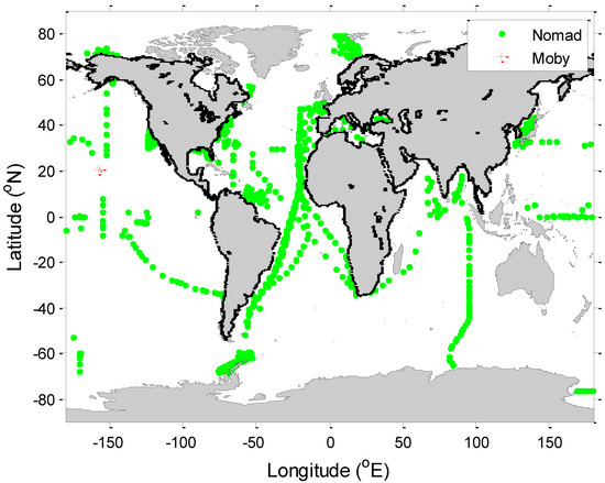
Figure 1.
Sampling locations for Marine Optical BuoY (MOBY) and NASA bio-Optical Marine Algorithm Dataset (NOMAD) in situ measurements.
The accuracy of Rrs was also validated using NOMAD in situ datasets. NOMAD is a global collection of in situ measurements contributed by many organizations [5]. It includes radiometric and phytoplankton data with an additional set of IOP observations from 1991 to 2007. The data were downloaded from the website (http://seabass.gsfc.nasa.gov/seabasscgi/nomad). The NOMAD-2008 data consisting of 3402 samples were used for the validation (sampling locations shown in Figure 1).
3. Results
3.1. Comparison of the Coverage of the Water-Leaving Reflectance between the LRSAC and the Standard Products
A sample of the one-day image (15 September 1998) of Rrs obtained from the LRSAC model was selected to compare with that of the SeaWiFS standard products downloaded from the websites, as shown in Figure 2. The image is a composite Rrs from about 14 tracks of satellite data measured on the same day in the range of the latitude between 45° N to 45° S. The pixel spatial resolution of both images is the same (about 9 ∗ 9 km2). The coverage of valid data in these two images is significantly different. There are ~28,800 valid pixels in Figure 2a while only ~8600 pixels in Figure 2b, indicating that LRSAC produces valid data about 2.4 times more than the standard products.

Figure 2.
A comparison of daily composite images of remote-sensing reflectance (Rrs) at Band 1 between (a) the layer removal scheme for atmospheric correction (LRSAC) model and (b) the standard product on 15 September 1998. The magnitudes of image pixels are indicated by the color bar with the unit of sr−1. Cloudy areas and invalid pixels are masked black and land white.
The difference of valid pixels in Figure 2 is mainly due to the cloud mask scheme. Normally, an epsilon value is computed from the ratio of AOD in two near-infrared bands and used to match the aerosol models. We used the epsilon spectrum to match the aerosol models for the LRSAC [22], and the values of Rrs at the two NIR bands can still be obtained and used for cloud mask. Clouds were masked by the values in Band 8 larger than 0.005 sr−1 for oceanic waters. For turbid waters, the threshold is modified (>0.02 sr−1 for Band 8 and >0.025 sr−1 for Band 1). Therefore, the scheme of cloud mask without the threshold of AOD value leads to a significant increase in the coverage of valid pixels.
A comparison of the eight-day composite global images is shown in Figure 3. The number of valid pixels in the LRSAC image is significantly greater than the standard products (~68.1 vs. ~40.0 thousands). The LRSAC image occupies 95% of the valid pixels while the standard product is 56%. It is obvious that there are many large areas filled with empty for the standard eight-day composite images, as high AOD distributions over the oceans from the Saharan dust can last for a period of time [19]. In comparison, most areas have been recovered with valid pixels by the LRSAC. Therefore, the LRSAC model can greatly improve the coverage of valid pixels of the Rrs images.

Figure 3.
A comparison of eight-day composite Rrs images at Band 1 between (a) the LRSAC model and (b) the standard product during the Julian days of 257 to 264, 1998. The values of image pixels are indicated by the color bar with the unit of sr−1. Cloudy areas and invalid pixels are masked black and land white.
3.2. Validation of the Accuracy of the LRSAC Model
The accuracy of Rrs obtained by the LRSAC was assessed using the MOBY data. The MOBY data provide a wonderful in situ dataset to evaluate the accuracy of the satellite-retrieved Rrs, because the same instruments have been used for the daily measurements of the Rrs at the same location and the same local time, since 1997. MOBY measured the Rrs three times a day at around 11:00, 12:00, and 13:00 local time, and SeaWiFS measured this location at around 12:00 local time, therefore, the time window of these measurements on the same day were all met within ±3 h. The Rrs values of MOBY measured at 12:00 were converted to the values of six bands according to the band response function of SeaWiFS. As the coverage of one pixel is much larger than that of in situ measurements, the box of one pixel was used to establish the matchup dataset. A total of 1981 pairs between SeaWiFS and MOBY was obtained and are shown in Figure 4. All matchups were displayed to examine the robustness of the algorithm.

Figure 4.
Validation of sea-viewing wide field-of-view sensor (SeaWiFS) retrieved Rrs obtained by the LRSAC using MOBY measurements. A total of 1981 matchup pairs were found, and all pairs were displayed in the figure. The number in the color bars indicates the density of dots. Subfigures (a–f) represent the values in Bands 1 to 6 of SeaWiFS, respectively.
As shown in Figure 4, most points fall around the 1:1 line, which indicate that the satellite-retrieved Rrs, obtained by LRSAC, agree reasonably well with those from the MOBY measurements. All of the subfigures exhibit a concentrated cluster of data pairs, and their centers are located at the 1:1 line indicating that systematic errors of the satellite-retrieved Rrs are relatively small.
All pairs are displayed in Figure 4, showing there are some dots beyond the 1:1 line with their relative errors higher than 100%. These dots were taken as the outliers in the data quality control criteria. Finding outliers in the validation of Rrs is common because they can significantly blur the statistics results. For example, only seven pairs were found between the Moderate Resolution Imaging Spectroradiometer and Marine Optical Buoy System in 2003 [35]. During the 10 months of deployment of the Plymouth Marine Bio-Optical Databuoy, only about 6% of the potential matched pairs met the rigorous quality control criteria resulting in only 15 pairs for comparison [3]. Here, pairs with an absolute relative error higher than 100% were excluded to compute the mean relative error (MRE) and the mean absolute relative error (ARE), as shown in Table 1, but all pairs were used to compute other parameters including the root mean square error (RMSE).

Table 1.
Comparison of the Rrs between LRSAC-retrieval (Rsat) and MOBY measurements (Rm).
As can be seen in Table 1, for the six bands, the mean and STD values of the satellite-retrieved Rrs are consistent with those of the MOBY measurements. Both STD values of Rrs are relatively small with about 10% of the mean values, indicating that the seasonal variation of Rrs at the MOBY site is very small. The MRE values vary from –1.5% in Band 1 to 22.0% in Band 6, with a mean value of 7.9%. The large value of the MRE in Band 6 is due to some pairs with very small magnitudes of in situ data, but the RMSE value is still the smallest (0.00032 sr−1) among the six bands. There is approximately 20% variation in the ARE values vary, for Bands 1 to 5, with the exception of a large value in Band 6. It is also caused by the small magnitude of MOBY measurements in this band. The maximum of the RMSE values is 0.00191 sr−1 in Band 1 and the average is 0.00099 sr−1.
The buoy can only validate a narrow range of Rrs at a fixed location. A comprehensive dataset of in situ measurements covering a wide range of oceanographic conditions is essential for the validation [5]. Normally, a window of ±3 h was assumed to be acceptable for homogeneous water masses and reasonably stable atmospheric conditions [36]. The sites of the NOMAD dataset cover a wide distribution around the global oceans including the coastal and oceanic waters and a strict data quality control has been used to ensure the accuracy of Rrs, providing a consistent dataset to establish matchups for evaluating the accuracy of SeaWiFS data. The window of ±3 h and the box of one pixel were used to establish the matchup dataset including a total of 817 pairs. All pairs are shown in Figure 5.

Figure 5.
Validation of Rrs values retrieved by the LRSAC model using the NOMAD data. A total of 817 matchup pairs were found with the time window of ±3 h and the box of one pixel. All pairs are displayed in the figure to demonstrate the performance of the algorithm. Subfigures (a–f) represent values in Bands 1 to 6 of SeaWiFS, respectively. The number in the color bars indicates the density of dots.
Figure 5 shows that most points fall around the 1:1 line and data cluster centers are also located on the 1:1 line. Some matchups are beyond the 1:1 line and their relative errors are also high (>100%). Especially, there are some pairs with infinity values of the relative error due to zero values of in situ data in Band 6, leading to an invalid value of MRE. These pairs were taken as outliers to compute the MRE and ARE, shown in Table 2.
Table 2.
Comparison of ratio of radiance to irradiance (RRI) between the LRSAC-retrievals and NOMAD measurements.
As shown in Table 2, for all six bands, the mean and STD values of the two Rrs values are close to each other, which indicate a small systematic bias for the satellite-retrieved Rrs. The MRE values vary from –0.04% (Band 5) to 5.6% (Band 2), with a mean value of 2.1%. ARE values vary from 23.15% (Band 3) to 40.56% (Band 6), with a mean value of 29.23%. The RMSE values in all six bands are very close to each other with a mean value of 0.0025 sr−1. From the validation of MOBY and NOMAD, the accuracy of the LRSAC model is quite satisfactory for the SeaWiFS global data.
Normally, the accuracy of Rrs is affected by the presence of high AOD and this is the reason the threshold of AOD is set to mask as invalid pixels for data quality control. Noteably, it was still to be determined whether the accuracy of the satellite-retrieved Rrs, obtained by LRSAC, is affected in the presence of high AOD. To address this issue, the MOBY matchups are grouped according to the different ranges of AOD and RMSE values are computed to evaluate the accuracy of Rrs related with the increase of AOD, as shown in Figure 6. The matchups are sorted by the increase of AOD values and each 10 continuous pairs are taken as one group to obtain the RMSE and the average of AOD. A total of 198 RMSE values was obtained from 1981 pairs of MOBY matchup dataset and their variations can be used to evaluate the relationship between the accuracy of LRSAC and the increase of AOD.

Figure 6.
The comparison of root mean square error (RMSE) values of SeaWiFS-retrieved Rrs between LRSAC (black dots) and standard products (red dots) with an increase of aerosol optical depth (AOD) values at 555 nm. Both are validated by MOBY measurements. Subfigures (a–f) represent SeaWiFS Bands 1 to 6, respectively.
Figure 6 shows that the variations of RMSE with the increase of AOD values are different among the six bands. The averages of RMSE decrease with longer wavelengths of the bands and they are related to the magnitudes of Rrs at the MOBY site. The values of RMSE vary around 0.002 sr−1 in Band 1, while they are about 0.0002 sr−1 in Band 6. These values of each band vary around the mean value when the AOD values change from 0.025 to 0.45. The RMSE variations from the standard products show similar trends with an increase of AOD. Therefore, the presence of high AOD did not significantly affect the accuracy of Rrs values in the atmospheric correction of the LRSAC, while the coverage of valid pixels of Rrs is significantly improved.
4. Discussion
4.1. The Relationship between the Valid Coverage of Rrs and AOD Values for the LRSAC Model
The SeaDAS software has been widely used to produce regional and global ocean color products such as the Rrs and chlorophyll-a concentrations from satellite data. Over the past decades, its performance has been significantly improved for processing the satellite ocean color data, but the coverage of valid pixels is still low. In contrast, the LRSAC has significantly improved the coverage of SeaWiFS-retrieved images. To compare the coverage of images between the LRSAC and the standard products, the number of valid pixels were computed on the daily images of Rrs over the ocean regions, as shown in Figure 7. This amount was converted to the percentage of valid pixels using the ratio of the number of valid pixels to the total pixels of the ocean areas with the latitude range of 45° N to 45° S.

Figure 7.
The valid pixels computed from the coverage of the daily images of Rrs in SeaWiFS Band 1 in the ocean regions between 45° N to 45° S with (a) for the LRSAC and (b) for the standard products.
The valid pixels of the daily Rrs images of the LRSAC show seasonal variations with a mean value of 30.5%. Most values vary between 27% and 37% and values less than 27% in Figure 7a are caused by some SeaWiFS L1B lost files in the daily composite data. In contrast, the values of the standard products vary between 9% and 15% with a mean value of 11.5%. The ratio of the mean number of valid pixels between the two algorithms is 2.65, indicating that the LRSAC can retrieve the water-leaving reflectance with about 1.65 times more valid pixels than that of the standard products. This improvement stems from the removal of the AOD threshold setting to flag invalid data of Rrs and the different scheme of the atmospheric correction. Therefore, the coverage of valid pixels for SeaWiFS data can be significantly increased.
To understand the spatial distribution of valid pixels in different regions, the mean valid pixel coverage was calculated from the total SeaWiFS data during the period from 1997 to 2010, as shown in Figure 8. The values were computed from the number of valid pixels divided by the total number of pixels for each pixel of the satellite imagery with the unit of percent. The magnitudes of the two images are significantly different with the values of LRSAC higher than those of the standard products for all oceanic pixels. As the latitude region is limited within 45° N to 45° S, the solar zenith angles at the local noon time are all within the valid range of the atmospheric correction over the whole year. Therefore, the spatial structures of the images are not caused by the variations of solar zenith angles at the time of SeaWiFS data acquisition.

Figure 8.
The spatial distribution of the mean valid pixel coverage from the total SeaWiFS data during the period of 1997 to 2010 for (a) the LRSAC and (b) the standard products. The values are indicated by the color bar with the unit (%). The land is masked by white.
As the presence of cloud and high AOD is the main cause producing the invalid pixels, the structure of the valid image is directly related to the spatial-temporal inhomogeneity of clouds and high AOD. The valid pixel coverage of daily standard SeaWiFS-retrieved Rrs is very low, moreover the spatial distribution of valid pixels is also inhomogeneous with many regions below 5% during the period from 1997 to 2010. It indicates that the valid pixels can be obtained on only a few days during the whole year. In contrast, the coverage of valid pixels has been significantly increased by the LRSAC. The maxima of valid pixels can reach 45% in some oceanic waters, indicating that the LRSAC can retrieve almost half of the Rrs values from SeaWiFS data in these regions.
The ratio of the mean valid pixels between the LRSAC and the standard products, as shown in Figure 9, demonstrate the performance of the LRSAC in the presence of high AOD values. The maxima of the ratio can reach up to 10 and the values are higher than three in about 33.8% of ocean. These areas are normally presented with high AOD distributions. The minima of the ratio image are 1.2, indicating that the LRSAC increases the coverage of valid pixels in all ocean waters between 45° N and 45° S. To understand the relationship between the ratio of the valid pixels of Rrs and AOD values, the mean values of AOD obtained from SeaWiFS data in 1998 were computed, as shown in Figure 9b.

Figure 9.
The comparison between the ratio of the mean valid pixels of Rrs and mean AOD values. The land is masked by white. (a) The ratio of the mean valid pixels from the LRSAC to that from the standard products. (b) The mean AOD values at 555 nm obtained by the LRSAC from SeaWiFS data in 1998.
The mean AOD values show significant spatial inhomogeneity. The high AOD values in the China Sea are partly caused by the presence of high turbid waters which can be wrongly taken as the aerosol signals in the atmospheric correction procedure. A. comparison of the two images in Figure 9, shows that the spatial structures of large values are similar in many regions. It indicates that most of the high ratio values come from the regions with the AOD values higher than the average. The LRSAC can recover more valid pixels with an increase of AOD as compared with the standard products. Therefore, the LRSAC can significantly increase the coverage of valid pixels even in the presence of high AOD values.
4.2. The Relationship between the Valid Coverage of Rrs and the Threshold of AOD Maxima for SeaDAS
Normally, the valid coverage of Rrs is related to the threshold settings. We hope to know the increase of valid coverage with different thresholds of AOD. The default value of tauamax is 0.3 and now it is set as 1.0 to run SeaDAS to process the same SeaWiFS data. Other settings are still the same as the default. The Rrs image at Band 1 is shown in Figure 10a, together with the eight-day composite image at Band 1 in Figure 10b.

Figure 10.
The SeaWiFS Rrs image of one day on September 15, 1998 (a) and 8-day composite images during days 257 to 264, 1998 at Band 1 (b) produced by SeaWiFS data analysis system (SeaDAS) with the tauamax of 1.0. The values of image pixels are indicated by the color bar with the unit of sr−1. Cloudy areas and invalid pixels are masked black and land white.
Comparing Figure 10a with Figure 2b, the valid coverage of Rrs has been increased when the threshold of tauamax is set as 1.0 for SeaDAS. This value is big enough to be taken as the removal of AOD to mask the Rrs product. The increase of valid coverage of Rrs is also indicated by the comparison of the images between Figure 10b and Figure 3b. However, the increase of valid pixels in the presence of high AOD values is still limited, as shown when Figure 10b is compared with Figure 3a. Therefore, the scheme of atmospheric correction for the LRSAC benefits to increase the number of valid pixels in th presence of high aerosol loads. But the accuracy of Rrs still needs to be further evaluated and other suitable threshold settings need to be developed to ensure the data quality of Rrs.
4.3. The Accuracy of the Standard SeaWiFS Products
The values of Rrs between the two images in Figure 2 are also different in the pixel-by-pixel comparison. The accuracy of the standard products was assessed based on the MOBY data. The same criteria for LRSAC and MOBY were used to establish the matchup dataset. A total of 1081 pairs were obtained, and the comparison is shown in Figure 11. It is clear that the scattered dots in each subfigure have one cluster center but the centers for Bands 1 to 3 deviate from the 1:1 line, which indicates that the values of the standard Rrs products have been slightly overestimated.
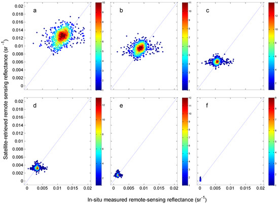
Figure 11.
Validation of the standard Rrs products using the MOBY measurements. The number in the color bars indicates the density of dots. Subfigures (a–f) represent the values in Bands 1 to 6 of SeaWiFS, respectively.
To evaluate the stability of the satellite-retrieved products, the daily Rrs values obtained by two kinds of satellite-retrieved Rrs at Band 1 were compared with MOBY measurements, as shown in Figure 12. It demonstrates the Rrs difference for daily measurements between MOBY and standard products.

Figure 12.
Comparison of Rrs at Band 1 among the measurements of MOBY (black) and the standard products (red). Their mean values are represented by the black and red lines for each year. Each subfigure represents results in one year from 1998 to 2009.
The yearly MRE values are computed with the values of −0.9%, 9.3%, 9.0%, 8.9%, 2.5%, 6.1%, 12.4%, 10.2%, 9.9%, 6.2%, 10.2%, 5.8%, 6.3%, and 13.3% for the years from 1997 to 2010. The mean of yearly MRE of the standard products is 7.8%. Therefore, the accuracy of atmospheric correction for the standard products needs to be improved.
The accuracy of SeaWiFS at other bands are also evaluated by the measurements at MOBY site. The MRE, ARE, and RMSE at six bands are listed in Table 3, together with these values evaluated by the measurements of NOMAD. The same rules for Table 1 are used to mask outliers to compute the MRE and ARE.
Table 3.
The accuracy of standard SeaWiFS Rrs valuated by MOBY and NOMAD measurements.
From Table 3, the MRE values of standard products vary around 9% for the six bands valuated by MOBY measurements. They are all positive but most MRE values are negative valuated by NOMAD. The evaluation results of satellite-retrieved products normally change with different datasets of in situ measurements. The accuracy of in situ data is important in evaluating the data quality of satellite products. The magnitudes of MRE from MOBY are bigger than those from NOMAD but ARE values of MOBY are smaller than those of NOMAD. The results of RMSE are similar to those of ARE.
5. Conclusions
The LRSAC model uses a nonlinear approach for ocean color atmospheric correction based on a five-layer structure in the Sun-Earth-satellite system. The nonlinear approach includes the multiple scattering effects of the interface between two layers such as the Rayleigh aerosol and other interactions. A step-by-step procedure can remove the effects of each layer, clearly decoupled each component from the satellite-received radiance. The atmospheric transmittance is portioned into the following three parts: atmospheric absorbance, Rayleigh, and aerosols. The transmittance of each layer is computed based on the transmittance of upwelling radiance and the transmittance of downwelling irradiance. Therefore, the LRSAC provides a new scheme for the atmospheric correction of satellite ocean color data.
Comparing the coverage of valid pixels in two daily Rrs images between the LRSAC and the standard SeaWiFS products downloaded from the web revealed that the number of valid pixels can significantly increase by up to 2.4 times. The comparison of the mean number of the valid pixels of the daily images obtained by the LRSAC (30.5%) and that of the standard products (11.5%) during the period from 1997 to 2010, shows that the LRSAC can recover about 1.65 times more valid pixels than that of the standard products. The comparison of two eight-day composite images also demonstrated that many regions filled with empty values in the standard products can be recovered by the LRSAC due to the presence of high AOD. From the comparison of the ratio of mean valid pixels with the mean AOD values, the LRSAC can recover the valid Rrs more than two times as compared with the standard products, in about 33.8% of oceanic regions. The increase of valid pixels benefited from the new scheme of the atmospheric correction and the removal of the AOD threshold to mask invalid pixels.
The accuracy of LRSAC-retrieved Rrs has been validated by in situ measurements from MOBY and NOMAD datasets. Both MOBY and NOMAD provide significant in situ Rrs for evaluating satellite-retrieved data with high data quality. The results show that most matchup pairs of the Rrs from the LRSAC and MOBY focused around the 1:1 line for the SeaWiFS six visible bands, indicating a small RMSE with a mean of 0.00099 sr−1. The centers of matchup clusters are all located at the 1:1 line, indicating a small systematic bias of the Rrs with a mean MRE value of 7.9%. Comparing the Rrs between the LRSAC and NOMAD, most matchup pairs are also distributed around the 1:1 line with a mean MRE value of 2.1% and the RMSE is 0.0025 sr−1. The accuracy of the LRSAC was also evaluated according to the increase of AOD values, demonstrating that the performance of the LRSAC is not significantly affected by the presence of high AOD. The positive validation results indicate that the LRSAC model is a reliable method for atmospheric correction to process the SeaWiFS global data, especially in the presence of high AOD.
Author Contributions
Conceptualization, Z.M.; methodology, B.T.; software, P.C.; validation, J.C.; formal analysis, Z.H.; investigation, Q.Z.; resources, J.C.; data curation, B.T.; writing—original draft preparation, Z.M.; writing—review and editing, Z.M.; visualization, P.C.; supervision, Z.M.; project administration, H.H.; funding acquisition, H.H. All authors have read and agreed to the published version of the manuscript.
Funding
This study was supported by the National Key Research and Development Program of China (2016YFC1400901), the National Science Foundation of China (61991454, 41621064, 41476156), and the Major project of High-Resolution Earth Observation Systems of National Science and Technology (05-Y30B01-9001-19/20-2).
Acknowledgments
We would like to thank organizations who provided in situ measurements and satellite remote sensing data. We thank Cho-Teng Liu of the National Taiwan University, Yan Li of the Xiamen University, Palanisamy Shanmugam of the Indian Institute of Technology Madras, and Knut Stamnes of the Stevens Institute of Technology for their suggestions and help to improve the manuscript. Two anonymous reviewers provided useful comments and criticism, which helped to improve it significantly.
Conflicts of Interest
The authors declare no conflict of interest.
References
- Gordon, H.R. Removal of atmospheric effects from the satellite imagery of the oceans. Appl. Opt. 1978, 17, 1631–1636. [Google Scholar] [CrossRef] [PubMed]
- Wang, M. An efficient method for multiple radiative transfer computations and the lookup table generation. J. Quant. Spectr. Rad. Trans. 2003, 78, 471–480. [Google Scholar] [CrossRef]
- Pinkerton, H.M.; Lavender, S.J.; Aiken, J. Validation of SeaWiFS ocean color satellite data using a moored data buoy. J. Geophy. Res. Oceans 2003, 108. [Google Scholar] [CrossRef]
- Jamet, C.; Loisel, H.; Kuchinke, C.P.; Ruddick, K.; Zibordi, G.; Feng, H. Comparison of three SeaWiFS atmospheric correction algorithms for turbid waters using AERONET-OC measurements. Remote Sens. Environ. 2011, 115, 1955–1965. [Google Scholar] [CrossRef]
- Werdell, P.J.; Bailey, S.W. An improved in-situ bio-optical data set for ocean color algorithm development and satellite data product validation. Remote Sens. Environ. 2005, 98, 122–140. [Google Scholar] [CrossRef]
- Hu, C.; Feng, L.; Lee, Z. Uncertainties of SeaWiFS and MODIS remote sensing reflectance: Implications from clear water measurements. Remote Sens. Environ. 2013, 133, 168–182. [Google Scholar] [CrossRef]
- Harmel, T.; Chami, M. Estimation of daily photosynthetically active radiation (PAR) in presence of low to high aerosol loads: Application to OLCI-like satellite data. Opt. Express 2016, 24, A1390–A1407. [Google Scholar] [CrossRef]
- Tripathy, M.; Raman, M.; Chauhan, P. Modulation in Ocean Primary Production due to Variability of Photosynthetically Available Radiation under Different Atmospheric Conditions. Int. J. Oceanol. 2014, 2014, 279412. [Google Scholar] [CrossRef]
- Steinmetz, F.; Deschamps, P.Y.; Ramon, D. Atmospheric correction in presence of sun glint: Application to MERIS. Opt. Express 2011, 19, 9783–9800. [Google Scholar] [CrossRef]
- Gordon, H.R.; Castaño, D.J. Coastal Zone Color Scanner atmospheric correction algorithm: Multiple scattering effects. Appl. Opt. 1987, 26, 2111–2122. [Google Scholar] [CrossRef]
- Gordon, H.R.; Wang, M. Retrieval of water-leaving radiance and aerosol optical thickness over the oceans with SeaWiFS: A preliminary algorithm. Appl. Opt. 1994, 33, 443–452. [Google Scholar] [CrossRef] [PubMed]
- Gordon, H.R.; Wang, M. Surface-roughness considerations for atmospheric correction of ocean color sensors. II: Error in the retrieved water-leaving radiance. Appl. Opt. 1992, 31, 4261–4267. [Google Scholar] [PubMed]
- Wang, M. The Rayleigh lookup tables for the SeaWiFS data processing: Accounting for the effects of ocean surface roughness. Int. J. Remote Sens. 2002, 23, 2693–2702. [Google Scholar] [CrossRef]
- Wang, M. A refinement for the Rayleigh radiance computation with variation of the atmospheric pressure. Int. J. Remote Sens. 2005, 26, 5651–5663. [Google Scholar] [CrossRef]
- Siegel, D.A.; Wang, M.; Maritorena, S.; Robinson, W. Atmospheric correction of satellite ocean color imagery: The black pixel assumption. Appl. Opt. 2000, 39, 3582–3591. [Google Scholar] [CrossRef] [PubMed]
- Ding, K.; Gordon, H.R. Analysis of the influence of A-band absorption on atmospheric correction of ocean color imagery. Appl. Opt. 1995, 34, 2068–2080. [Google Scholar] [CrossRef] [PubMed]
- Domsta, J. Radiance reflectance of homogeneous plane parallel layers. Oceanologia 1993, 34, 5–12. [Google Scholar]
- Gordon, H.R.; Castaño, D.J. Aerosol analysis with the Coastal Zone Color Scanner: A simple method for including multiple scattering effects. Appl. Opt. 1989, 28, 1320–1326. [Google Scholar] [CrossRef]
- Wang, M. Aerosol polarization effects on atmospheric correction and aerosol retrievals in ocean color remote sensing. Appl. Opt. 2006, 45, 8951–8963. [Google Scholar] [CrossRef]
- Moulin, C.; Gordon, H.R.; Chomko, R.M.; Banzon, V.F.; Evan, R.H. Atmospheric correction of ocean color imagery through thick layers of Saharan dust. Geophy. Res. Lett. 2001, 28, 5–8. [Google Scholar] [CrossRef]
- Shanmugan, P.; Ahn, Y. New atmospheric correction technique to retrieve the ocean colour from SeaWiFS imagery in complex coastal waters. J. Opt. A Pure Appl. Opt. 2007, 9, 511–530. [Google Scholar] [CrossRef]
- Bailey, S.W.; Franz, B.A.; Werdell, P.J. Estimations of near-infrared water-leaving reflectance for satellite ocean color data processing. Opt. Express 2010, 18, 7521–7527. [Google Scholar] [CrossRef] [PubMed]
- Mao, Z.; Pan, D.; Hao, Z.; Chen, J.; Tao, B.; Zhu, Q. A potentially universal algorithm for estimating aerosol scattering reflectance from satellite remote sensing data. Remote Sens. Environ. 2014, 142, 131–140. [Google Scholar] [CrossRef]
- Fan, Y.; Li, W.; Gatebe, C.K.; Jamet, C.; Zibordi, G.; Schroeder, T.; Stamnes, K. Atmospheric correction and aerosol retrieval over coastal waters using multilayer neural networks. Remote Sens. Environ. 2017, 199, 218–240. [Google Scholar] [CrossRef]
- Gordon, H.R. Radiative transfer: A technique for simulating the ocean in satellite remote sensing calculation. Appl. Opt. 1976, 15, 1974–1979. [Google Scholar] [CrossRef]
- Hu, B.; Lucht, W.; Strahler, A.H. The interrelationship of atmospheric correction of reflectances and surface BRDF retrieval: A sensitivity study. IEEE Trans. Geosci. Remote Sens. 1999, 37, 724–738. [Google Scholar]
- Gao, B.C.; Montes, M.J.; Ahmad, Z.; Davis, C.O. Atmospheric correction algorithm for hyperspectral remote sensing of ocean color from space. Appl. Opt. 2000, 39, 887–896. [Google Scholar] [CrossRef]
- Kokhanovsky, A.A.; Mayer, B.; Rozanov, V.V. A parameterization of the diffuse transmittance and reflectance for aerosol remote sensing problems. Atmos. Res. 2005, 73, 37–43. [Google Scholar] [CrossRef]
- Jiménez-Muñoz, J.C.; Sobrino, J.A.; Mattar, C.; Franch, B. Atmospheric correction of optical imagery from MODIS and Reanalysis atmospheric products. Remote Sens. Environ. 2010, 114, 2195–2210. [Google Scholar] [CrossRef]
- Bilal, M.; Nichol, J.E.; Bleiweiss, M.P.; Dubois, D. A Simplified high resolution MODIS Aerosol Retrieval Algorithm (SARA) for use over mixed surfaces. Remote Sens. Environ. 2013, 136, 135–145. [Google Scholar] [CrossRef]
- He, T.; Liang, S.; Wang, D.; Wu, H.; Yu, Y.; Wang, J. Estimation of surface albedo and directional reflectance from Moderate Resolution Imaging Spectroradiometer (MODIS) observations. Remote Sens. Environ. 2012, 119, 286–300. [Google Scholar] [CrossRef]
- Vermote, E.F.; Tanré, D.; Deuzé, J.L.; Herman, M.; Morcrette, J.J. Second Simulation of the Satellite Signal in the Solar Spectrum, 6S: An overview. IEEE Trans. Geosci. Remote Sens. 1997, 35, 675–686. [Google Scholar] [CrossRef]
- Lacis, A.A.; Hansen, J.E. A parameterization for the absorption of solar radiation in the Earth’s atmosphere. J. Atmos. Sci. 1974, 31, 118–133. [Google Scholar] [CrossRef]
- Wang, M. Atmospheric correction of ocean color sensors: Computing atmospheric diffuse transmittance. Appl. Opt. 1999, 38, 451–455. [Google Scholar] [CrossRef] [PubMed]
- Fraser, R.S.; Mattoo, S.; Yeh, E.N.; McClain, C.R. Algorithm for atmospheric and glint corrections of satellite measurements of ocean pigment. J. Geophy. Res. 1997, 102, 17107–17118. [Google Scholar] [CrossRef]
- Kotchenova, S.Y.; Vermote, E.F.; Matarrese, R.; Klemm, F.J. Validation of a vector version of the 6S radiative transfer code for atmospheric correction of satellite data. Part I: Path Radiance. Appl. Opt. 2006, 45, 6762–6774. [Google Scholar]
© 2019 by the authors. Licensee MDPI, Basel, Switzerland. This article is an open access article distributed under the terms and conditions of the Creative Commons Attribution (CC BY) license (http://creativecommons.org/licenses/by/4.0/).