Article

Feasibility of Burned Area Mapping Based on ICESAT−2 Photon Counting Data

Department of Ecosystem Science & Management, 534 John Kimbrough Blvd, Texas A&M University, College Station, TX 77843, USA
*
Author to whom correspondence should be addressed.
Remote Sens. 2020, 12(1), 24; https://doi.org/10.3390/rs12010024
Submission received: 21 November 2019 / Revised: 14 December 2019 / Accepted: 16 December 2019 / Published: 19 December 2019
(This article belongs to the Special Issue Lidar Remote Sensing of Forest Structure, Biomass and Dynamics)

Abstract

:
Accurately mapping burned areas is crucial for the analysis of carbon emissions and wildfire risk as well as understanding the effects of climate change on forest structure. Burned areas have predominantly been mapped using optical remote sensing images. However, the structural changes due to fire also offer opportunities for mapping burned areas using three-dimensional (3D) datasets such as Light detection and ranging (LiDAR). This study focuses on the feasibility of using photon counting LiDAR data from National Aeronautics and Space Administration’s (NASA) Ice, Cloud, and land Elevation Satellite-2 (ICESat−2) mission to differentiate vegetation structure in burned and unburned areas and ultimately classify burned areas along mapped ground tracks. The ICESat−2 mission (launched in September 2018) provides datasets such as geolocated photon data (ATL03), which comprises precise latitude, longitude and elevation of each point where a photon interacts with land surface, and derivative products such as the Land Water Vegetation Elevation product (ATL08), which comprises estimated terrain and canopy height information. For analysis, 24 metrics such as the average, median and standard deviation of canopy height were derived from ATL08 data over forests burned by recent fires in 2018 in northern California and western New Mexico. A reference burn map was derived from Sentinel−2 images based on the differenced Normalized Burn Ratio (dNBR) index. A landcover map based on Sentinel−2 images was employed to remove non-forest classes. Landsat 8 based dNBR image and landcover map were also used for comparison. Next, ICESat−2 data of forest samples were classified into burned and unburned ATL08 100-m segments by both Random Forest classification and logistic regression. Both Sentinel−2 derived and Landsat 8 derived ATL08 samples got high classification accuracy, 83% versus 76%. Moreover, the resulting classification accuracy by Random Forest and logistic regression reached 83% and 74%, respectively. Among the 24 ICESat−2 metrics, apparent surface reflectance and the number of canopy photons were the most important. Furthermore, burn severity of each ATL08 segment was also estimated with Random Forest regression. R2 of predicted burn severity to observed dNBR is 0.61 with significant linear relationship and moderate correlation (r = 0.78). Overall, the reasonably high accuracies achieved in this study demonstrate the feasibility of employing ICESat−2 data in burned forest classification, opening avenues for improved estimation of burned biomass and carbon emissions from a 3D perspective.

Graphical Abstract

1. Introduction

Wildfire related risk and damage have increased over the past three decades [1], causing threats to ecosystem function and human society. Currently, global warming and extreme droughts are contributing to increased wildfire activities [2]. Increased wildfires in return cause more warming effects through quick release of carbon sequestered in terrestrial ecosystems [3]. Wildfires play important roles in ecosystem succession, biogeochemical cycles and climate change. Thus, accurately mapping burned areas, serving as the basic step for wildfire management, is crucial for the analysis of carbon emissions and fire risk as well as understanding the effects of climate change on ecosystems.
Remotely sensed images have been used for mapping burned areas for decades [4,5]. Fire-induced changes such as vegetation removal, structure alteration and charcoal deposition all cause spectral shift that enable multispectral remote sensing techniques to be applied. To be specific, notable responses are observed in Near infrared (NIR) (decrease) and shortwave infrared (SWIR) bands (increase) [6]. Classification techniques like logistic regression [7] and object-based classification [8] have been proven to be effective in capturing spectral features of burned regions. Spectral indices like Normalized Burn Ratio (NBR) index [9] and differenced Normalized Burn Ratio (dNBR) index [10] are also commonly used to create burned maps. With improved availability of multitemporal remote sensing imagery, burned areas have also been mapped using time series analysis. Hawbaker et al. [11] produced long term burn area products in the conterminous United States with Landsat images. Roteta et al. [12] also used time series of Sentinel−2 A images to map burned areas in sub-Saharan Africa and the accuracy was claimed to be higher than that of the MODIS global fire product (MCD64 A1). However, remote sensing images are limited in capturing the three-dimensional (3D) vegetation structure, which makes it difficult to obtain under canopy fire information and canopy height measurement [13]. To provide more accurate estimation of fire severity, terrestrial carbon storage and biomass emissions, methods based on 3D data are essential to complement existing image-based approaches [14,15].
Light detection and ranging (LiDAR) offers an effective way of producing 3D structures, which has previously been applied for mapping burned areas and forest fuel types [16,17]. By measuring the time interval of transmitted and received energy, LiDAR can calculate the distance between LiDAR sensor and targets, providing information on the three-dimensional structure of vegetated ecosystems [18]. Thus, LiDAR can be used to monitor structure changes of vegetation caused by fires. Wang et al. [19] mapped burned areas based on height differences of sagebrush derived from pre- and post-fire airborne LiDAR data and classified the whole region into three levels of severity using height thresholds. Montealegre et al. [17] applied a logistic regression model to classify burned areas in Spanish forests based on post-fire airborne LiDAR data. Other studies, e.g., Garcia et al. [16] integrated post-fire airborne LiDAR data and Landsat images to map burned areas and estimate consumed biomass with high accuracy. While using airborne LiDAR data provides detailed vegetation structure with high accuracy, the application of these data over large areas is constrained by the high expense associated with data acquisition.
At regional and global scales, spaceborne LiDAR has been instrumental in capturing 3D data globally and efficiently with fixed footprint and revisit time, providing large coverage and repeatable observations [20,21]. A notable spaceborne LiDAR mission includes National Aeronautics and Space Administration’s (NASA) first Ice, Cloud, and land Elevation Satellite (ICESat) mission, which carried the Geoscience Laser Altimeter System (GLAS), which is a waveform LiDAR instrument, launched in January 2003. GLAS is the first spaceborne LiDAR sensor with the aim of measuring ice sheets globally [22]. The footprint of GLAS beams is 70 m and the along-track sampling distance is 172 m with a wavelength of 1064 nm [20]. GLAS records backward energy with waveform LiDAR measurement for each footprint. This mission stopped collecting data in October 2009, after providing billions of LiDAR waveform data for the analysis of ice, cloud and vegetation [16,23]. These waveform data were also employed to evaluate fire disturbance in Alaska forests [24], where structure changes of forests between burned and unburned areas were found to be significant. Moreover, García et al. [25] used GLAS data to characterize canopy fuels. However, the ICESat footprint, though unprecedented at the time, is quite coarse (70 m) which limited the resolution of finer 3D details.
As a follow-up mission to ICESat, ICESat−2 was launched on September 15 2018 with the Advanced Topographic Laser Altimeter System (ATLAS) [21,26]. ATLAS is a photon counting LiDAR with a footprint of 14 m and along-track sampling distance of 0.7 m, which presents a tremendous improvement in sampling compared to its predecessor. The ATLAS instrument measures the time a photon takes to travel from ATLAS to Earth and back so as to determine the photon’s geodetic latitude and longitude. Unlike single waveform beams in GLAS, ATLAS emits three pairs of beams with a wavelength of 532 nm. Each pair consists of a strong beam and weak beam using a transmit energy ratio of 4:1. The improved spatial resolution and coverage of ICESat−2 will better assist the mapping of ice and vegetation. One of ICESat−2’s data products is the Land and Vegetation height product (ATL08), which provides terrain and canopy height measurement at 100 m segments along the ground track. The ATL08 product provides various canopy and terrain related metrics such as mean canopy height, max canopy height, apparent surface reflectance, the number of canopy photons, the number of terrain photon and canopy openness in each segment. ATL08 also provides cloud masks to help clean and filter the data. This standard canopy product will facilitate forests assessment at global scales and promote carbon monitoring. In this study, ATL08 data are used to map burned areas, which, based on current literature, is the first attempt of using such data for this purpose.
Machine learning has shown great success in classification and discrimination of remote sensing data [27,28]. With the capability to model complex class signatures without statistical assumptions on data distribution (non-parametric) and the ability to process high-dimensional data, machine learning approaches are widely accepted [29]. Moreover, machine learning algorithms are more robust and produce higher classification accuracy than traditional parametric classifiers such as maximum likelihood [27,29]. Machine learning methods such as random forest [30], gradient boosted regression [11] and neural network have found application in various studies. Wu et al. [31] evaluated support vector machine, Random Forest and decision tree to classify point clouds to obtain canola canopy structures, concluding that Random Forest provides better results. Krishna Moorthy et al. [32] classified liana stems from point clouds by Random Forest with an accuracy of 88%. For this study, we used Random Forest to classify burned 100 m ATL08 photon segments and logistic regression is also included for comparison.
In this study, we investigated the application of ICESat−2 photon counting data for burned area mapping, which is the first attempt to employ spaceborne LiDAR in fire classification. Innovative aspects of this research include the use of machine learning methods with photon counting data to provide three-dimensional structural information along the satellite tracks. Optical images derived burn maps were used as references. Moreover, land cover maps were used to avoid interference of different land covers. The main goal was to investigate the feasibility of using ATL08 to map burned areas of wildfires. Our specific objectives were: (1) to develop a methodology for using ATL08 data for burned areas classification; (2) to compare the effects of Sentinel−2 and Landsat 8 images when used as reference images for identifying burned areas; (3) to compare the accuracy of different classification methods for ATL08 100 m-segments, like Random Forest and logistic regression; (4) to identify the most significant variables in ATL08 for classification of burned areas.

2. Materials and Methods
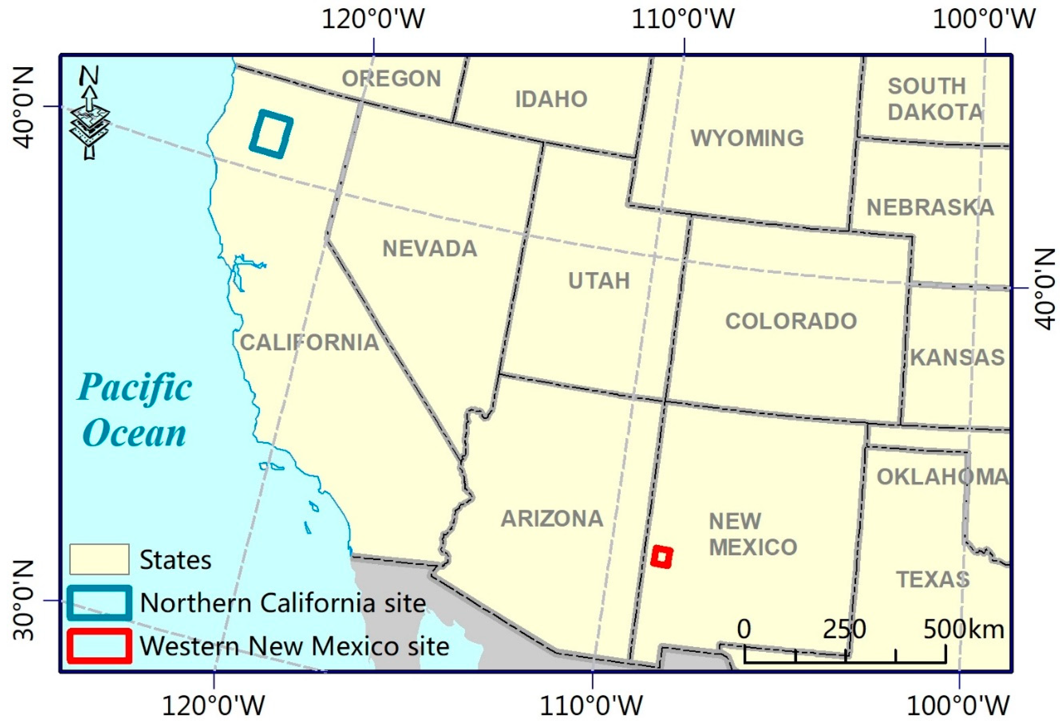
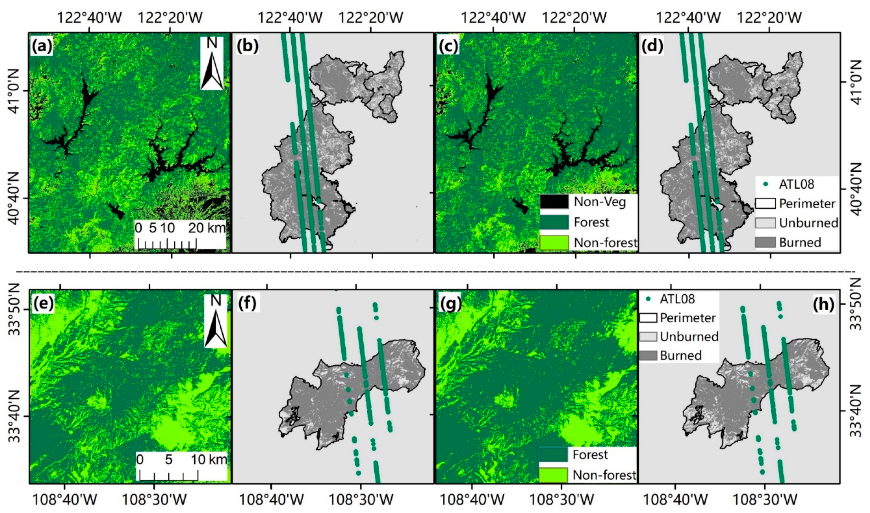
2.1. Study Area

Two study areas were chosen for burned area classification (Figure 1 and Figure 2). The first site is located in northern California. Two major fire events occurred over the study site (Figure 2b). The Carr Fire happened west of Shasta Lake, starting on July 23, 2018 until it was contained on August 30, 2018. The Delta Fire started on September 5, 2018 and stopped on October 7, 2018 in Shasta-Trinity National forest. The whole region is dominated by forests including ponderosa pine, canyon live oak and Douglas-fir with scattered shrubs, grasslands and bare grounds.
The second site is in Catron County, western New Mexico (Figure 1). Burn events on this site are mainly attributed to the Buzzard Fire, which burned parts of the Gila National Forest (Figure 2f). The Buzzard Fire occurred from May 22, 2018 until it was completely contained on June 24, 2018, after burning more than 20,000 hectares. This region is dominated by juniper, pine, aspen and spruce-fir forest areas of bare grounds.

2.2. Data

2.2.1. ATL08

ATL08 land and canopy height product is produced from ICESat−2 global geolocated photon data (ATL03), which include location (x, y, z) of each bounce point where photon interacts with land surface. In the following context, we use ‘location of photon’ to paraphrase ‘location of point where photon interacts with land surface’. Using the Differential, Regressive and Gaussian Adaptive Nearest Neighbor (DARGANN) algorithm, solar background noises in ATL03 are removed and signal photons are selected [33]. Then, the signal photons are filtered and classified into ground, canopy and top of canopy photons. Based on those classified photons, land and canopy structure related metrics are calculated and stored in ATL08 in h5 format. ATL08 data acquired on December 28, 2018 were downloaded for the northern California site from the National Snow & Ice Data Center (NSIDC) [34]. The full name of the data file is ‘ATL08_20181228195820_00060202_001_01.h5′. For the western New Mexico site, ATL08 data were acquired on October 21, 2018, as ATL08 data are only available from October 14, 2018. The file name is ‘ATL08_20181021221952_03560102_001_01.h5′. There were many metrics recorded for each 100 m segment and we used only the ones related to canopy three-dimensional structure (Table 1).
In h5 format, data were stored in several groups. ATL08 contains 10 major groups: metadata, ancillary_data, gt1 l, gt1 r, gt2 l, gt2 r, gt3 l, gt3 r, orbit_info and quality_assessment, where gt1 l means the left beam of ground track one, gt1 r means the right beam of ground track one and so forth. Six gtx groups contained height metrics of 100 m segments for ground tracks and the other four metadata related groups provided information on instrument, orbit and data quality [34]. The gtx group had two sub-groups: land_segments and signal_photons, where land_segments provided metrics and signal_photons provided information on corresponding ATL03 photons. Twenty-one metrics were obtained directly from ATL08 and three derived metrics were also employed (Table 1). For our analysis, only the three strong beams were employed, as they provided more vegetation photons. In ATL08 data, cloud obstructed segments and empty segments were filled by 3.4028 × 1038, which were discarded in this study.

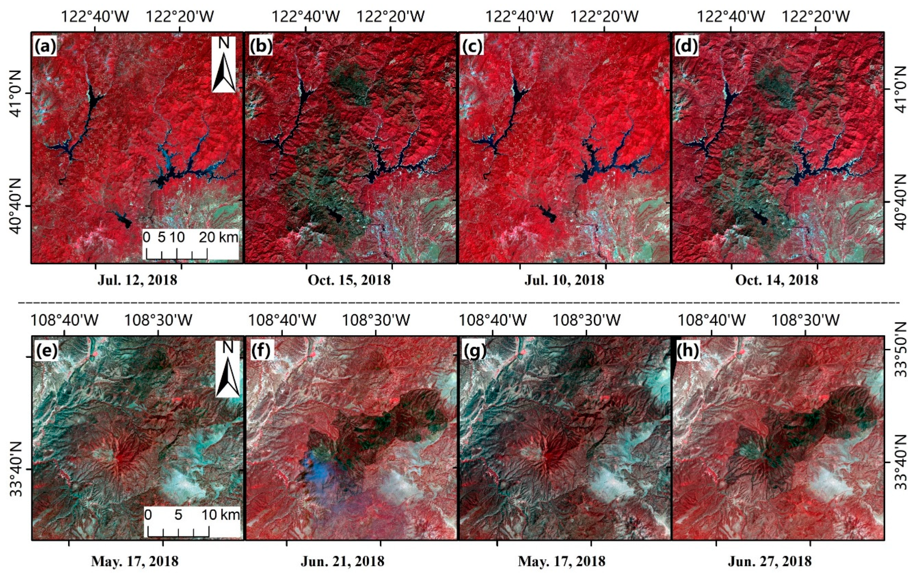
2.2.2. Sentinel and Landsat Data

Sentinel−2 Multi-Spectral Instrument (MSI) images pre- and post-fire were also downloaded from the United States Geological Survey (USGS) [35]. For the northern California site, the two images, one on July 12, 2018 and the other on October 15, 2018 (Figure 1), were atmospherically corrected by Sen2 Cor tool downloaded from the European Space Agency [36]. There are 13 bands in Sentinel−2 data with three different spatial resolutions: 10 m, 20 m and 60 m. Bands with 10 m resolution (B2, B3, B4 and B8) were selected (Table 2). The 20 m shortwave near infrared bands B11 and B12 (Table 2) were resized to 10 m using the nearest neighbor method. Then, these six bands were stacked and used in further processing. Landsat 8 Operational Land Imager (OLI) Analysis Ready Data (ARD) for July 10, 2018 (pre-fire) and October 14, 2018 (post-fire) were also downloaded from USGS. ARD contains surface reflectance of Landsat images from Landsat 4 to Landsat 8 and served for direct use in monitoring and assessing land cover changes. Similarly, the seven Landsat bands (B1 to B7) (Table 2) were stacked in the order of wavelength and used for later classification.
For the western New Mexico site, Sentinel−2 images on May 17, 2018 (pre-fire) and June 21, 2018 (post-fire) were downloaded. The fire was completely stopped on June 24, 2018 but there are no subsequent cloud free images after June 24 due to clouds. Therefore, the image on June 21 was used, which is acceptable, as most fires were contained before that day. Meanwhile, Landsat 8 ARD on May 17, 2018 (pre-fire) and June 27, 2018 (post-fire) were downloaded from USGS for comparison.

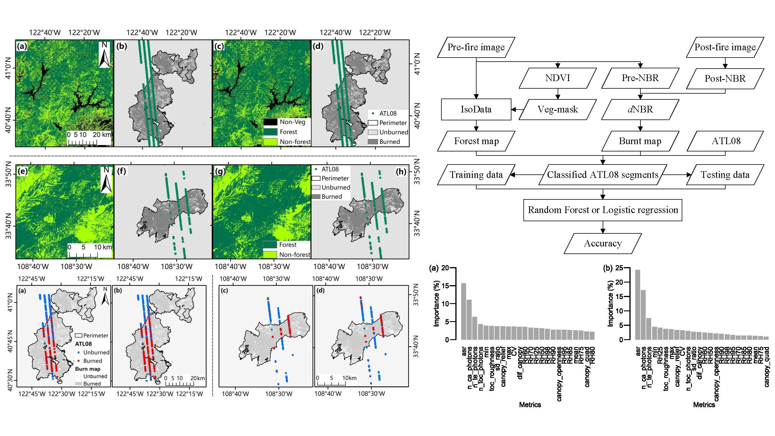
2.3. Forest Cover Mapping

To avoid the interference of different land covers, an accurate forest map is necessary. In the northern California site, normalized difference vegetation index (NDVI) values were calculated based on the pre-fire Sentinel−2 images. A threshold of 0.3, selected based on Otsu method [37], was used for northern California forests to mask non-vegetation pixels. Next, vegetation pixels were classified into 20 classes by the Iterative Self-Organizing Data Analysis Technique (IsoData) (Figure 3) in ENVI 5.5 (Harris Geospatial Solutions). Then, the 20 classes were merged into forest or non-forest types (Figure 4) based on Google Maps and visual interpretation. Finally, 200 random samples were created to assess classification accuracy based on visualization of each sample using Google Earth and pre-fire Sentinel−2 images, including 100 samples for the forest and another 100 samples for the non-forest areas. The overall accuracy turned out to be 88% and kappa was 0.76. The Landsat 8 OLI pre-fire image was also used to produce forest map of northern California with the same routine. The 200 random samples were employed to assess the accuracy of the OLI classification map. The overall accuracy of OLI forest map was 86% and kappa was 0.71, which are slightly lower than that of Sentinel−2. Table S1 in Supplemental materials shows that forest regions in Landsat 8 classification map are overestimated (row sum 126 larger than column sum 108), which is illustrated in Figure 4c.
In the New Mexico site, the Sentinel−2 image pre-fire was classified into 20 classes by IsoData and then merged into forest and non-forest based on visualization of Google map, pre- and post-fire images. Then, 200 random samples were used to check the classification accuracy. The same routine was employed on Landsat 8 data. Overall accuracy of Sentinel−2 forest map is 86.5% and kappa is 0.73. For Landsat 8 forest map, overall accuracy and kappa are 85% and 0.7035, respectively. Forest regions are overestimated in Landsat 8 map (Figure 4g) relative to Sentinel−2 map (Figure 4e). Confusion matrices are shown in Table S1 in Supplemental materials.
Then, both pre- and post-fire Sentinel−2 images were employed to produce reference burned areas map. First, Normalized Burn Ratio (NBR) (Equation (1)) indices were calculated based on pre-fire images and post-fire images separately. Next, the differenced NBR (dNBR) between pre-fire and post-fire data were derived. Fire perimeters downloaded from the Cal Fire (https://frap.fire.ca.gov/mapping/gis-data/) were used to mask out unburned pixels. Based on the suggested value from United States Geological Survey (USGS) [14,38], as shown in Table 3, a threshold of dNBR = 0.1 was further used to classify pixels into burned (>0.1) and unburned (<0.1) (Figure 4), removing those unburned islands within the fire perimeters. Landsat 8 images were also used to derive burned map in the same way. In total, 200 randomly created samples, 100 for burned regions and 100 for unburned regions, were employed to check the accuracy of burn map. Based on visual interpretation of each sample using Google Maps and post-fire images, overall accuracy of Sentinel−2 burn map is 85.5% and kappa is 0.71. For the Landsat 8 burn map, overall accuracy and kappa are 88.5% and 0.7676, respectively. Confusion matrices of burn maps are shown in Table S2 in the Supplemental materials.
In the western New Mexico site, a fire perimeter was downloaded from USGS (https://www.geomac.gov/GeoMACKML/getKML.aspx) to mask unburned pixels, and then, dNBR = 0.1 was used to remove unburned islands within fire perimeters with Sentinel−2 data and Landsat 8 data, respectively. In total, 200 randomly created samples, 100 for burned regions and 100 for unburned regions, were used to check accuracy of burn map. Based on visual interpretation of each sample using Google map and post-fire image, overall accuracy of Sentinel−2 burn map is 87.5% and kappa is 0.75. For the Landsat 8 burn map, overall accuracy and kappa are 87.5% and 0.7465, respectively. Confusion matrices of burn maps are shown in Table S2 in Supplemental materials.
{ NBR = NIR SWIR 2 NIR + SWIR 2 dNBR = NBR pre-fire NBR post-fire
where NIR means near infrared bands (B8 in Sentinel−2 or B5 in Landsat 8), SWIR2 (B12 in Sentinel−2 or B7 in Landsat 8) means shortwave infrared bands. Dates of pre-fire and post-fire images are described in Section 2.2.2.
For the northern California forest region, ATL08 segments locating between 40.480 N and 41.049 N were selected to cover both burned and unburned forests, as higher latitudes were snow covered. When overlaying forest map derived from optical images with ATL08 segments, a segment was regarded as forest segment if over 90% of pixels within it (a pixel will be counted even though only part of it is within the segment) were forest type. The segment was defined as non-forest type when over 90% of pixels were non-forest. The same rule was applied to the burned map. In the western New Mexico site, ATL08 segments within 33.55 N and 33.85 N were selected, as forests are dominant within the region. Due to the existence of outliers, a range of µ ± 2σ was employed to remove extreme values for each metric, where µ is the average and σ is the standard deviation. There are 592 forest segments (417 in northern California and 175 in western New Mexico) in total based on the Sentinel−2 forest map and burn map and 744 forest segments (551 in northern California and 193 in western New Mexico) using Landsat 8 data, combining the two study areas.

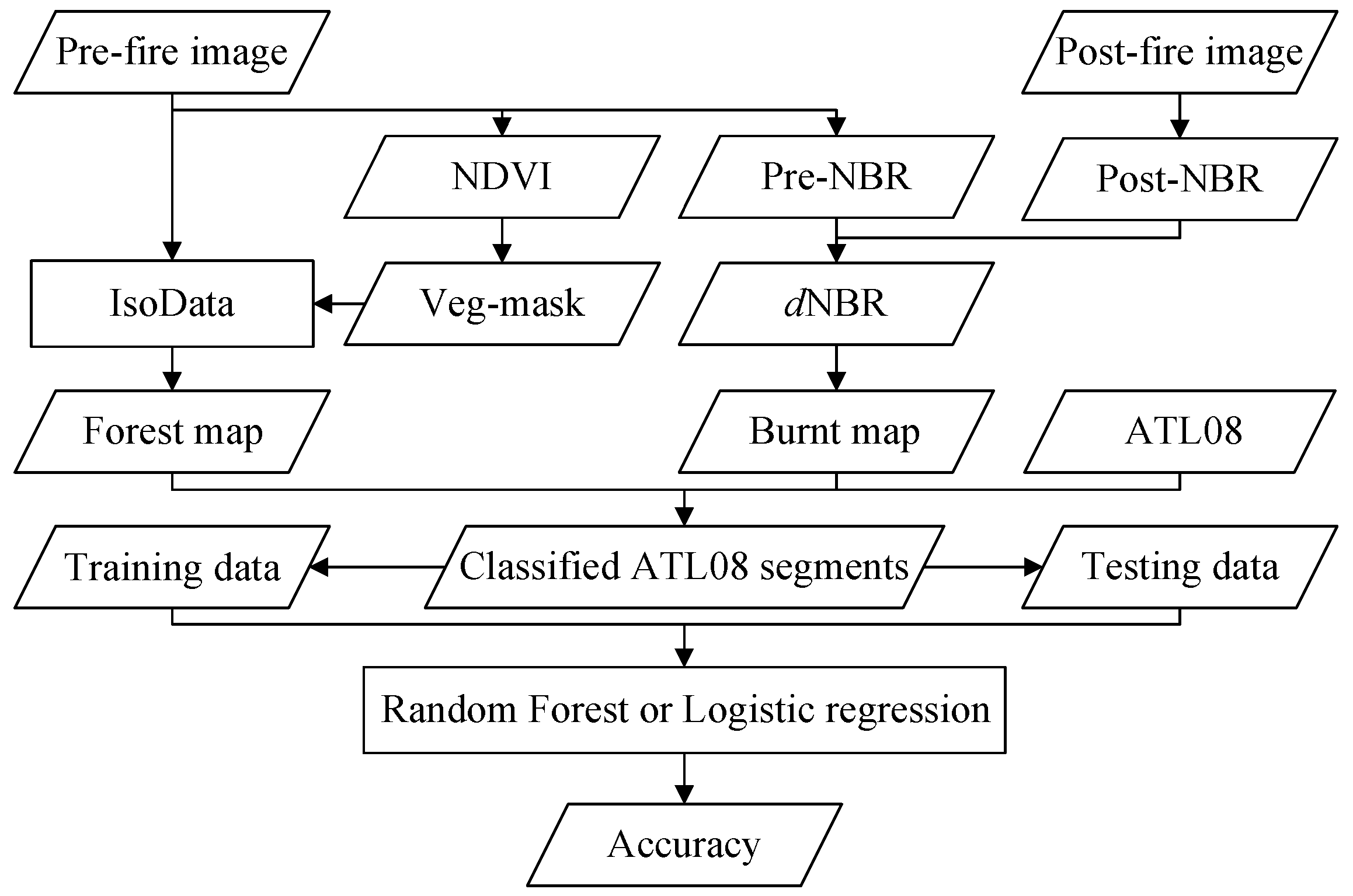
2.4. Fitting Models for Burned Area Mapping

2.4.1. Fitting Random Forest Model

The 24 canopy related LiDAR metrics were used as independent variables in building models for classifying burned areas. The dependent variable was the burn condition and was modeled as a binary variable (burned = 1, unburned = 0). Total ATL08 forest segments from both sites were randomly divided into two groups, 70% for training and the rest, 30%, for testing. In total, 1000 trees were used in the training process in R package ‘randomForest’. The best number of splits, which means the best number of predictors in a subset, was determined by the minimum out of bag (OOB) error. In Sentinel−2 derived samples, 414 ATL08 segments were used for training and 178 segments for testing. For Landsat 8 derived samples, 521 segments were used for training and 223 segments for testing.
Random Forest model was also used to estimate burn severity (which is approximated by dNBR). At first, for each ATL08 segment, average dNBR of covered pixels was calculated. In total, 24 metrics were used as features and the average dNBR value was a response variable. Using 70% samples for training and 30% for testing, the accuracy of burn severity estimation by the trained model can be evaluated. Relative differenced NBR index (RdNBR) (=dNBR/sqrt(NBRpre-fire)) [39] was also employed in burn severity estimation to compare with dNBR.

2.4.2. Fitting Logistic Regression Model

Logistic regression, serving as a classical statistic model, is suitable for categorical variables such as burned and unburned. Rather than modeling a categorical variable Y directly, logistic regression models the probability that y belongs to a specific class. For example, for a dichotomous problem burned (y = 1) and unburned (y = 0), logistic function fits a S-shaped curve with variables x1, x2, ···, xn (Equation (2)). A default threshold of probability is 0.5. Therefore, when the fitted probability is higher than 0.5, we get y = 1, otherwise, y = 0. The ‘stats’ package in R was used to conduct a multi-variate logistic regression. Training samples were employed to estimate the coefficient of each predictor. A stepwise procedure based on mixed selection was utilized to remove those insignificant metrics. Then, testing samples were used for accuracy assessment.
p ( y = 1 | x 1 , x 2 , , x n ) = e α + β 1 x 1 + β 2 x 2 + + β n x n 1 + e α + β 1 x 1 + β 2 x 2 + + β n x n
where p(y = 1|x1, x2, ···, xn) means the probability of y = 1 given metrics x1, x2, ···, xn. α is intercept and β1, β2, ···, βn are coefficients corresponding to metrics.

3. Results

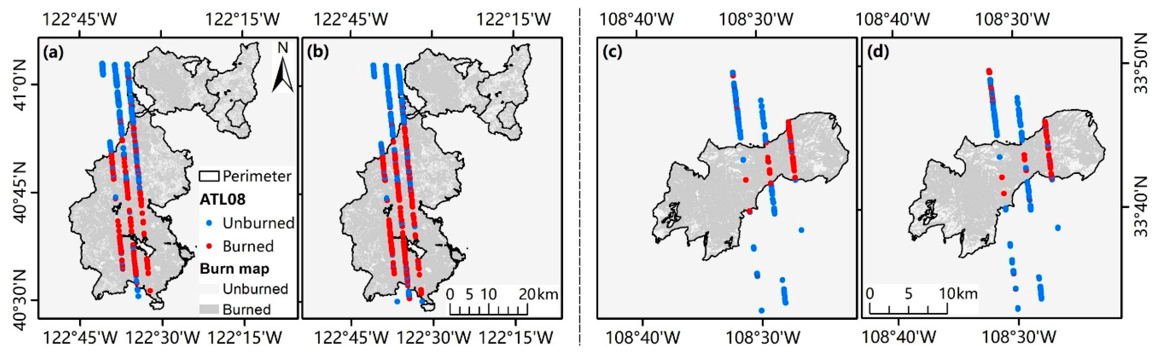
3.1. Burned Area Mapping by Random Forest

Figure 5 shows correlations of 24 LiDAR metrics of all Sentinel−2 derived samples in the northern California site and western New Mexico site. Basically, most metrics are significantly correlated with others, but the correlation coefficients vary greatly, which means metrics such as asr (apparent surface reflectance) and n_ca_photons (the number of canopy photons) still cannot replace each other. Moreover, most metrics are positively correlated with other metrics except asr, n_te_photons (the number of terrain photons), CV (coefficient of variation) and sd_ratio (standard deviation ratio). Canopy height related metrics such as RH25, RH50, RH60, RH70, RH75, RH80, RH85, RH90, RH95 and RH98 were highly correlated. However, metrics including dif_canopy (canopy difference to median height), min (minimum canopy height), n_ca_photons, n_toc_photons (the number of top of canopy photons), toc_roughness (top of canopy roughness), asr and n_te_photons have less correlation with other metrics, indicating splitting photon points into different types such as canopy photons, terrain photons and top of canopy photons provides extra information.
Figure 6 provides barplots of 24 metrics derived with Sentinel−2 forest maps and landcover maps from both study sites. Burned segments tend to have lower values than unburned segments except dif_canopy (canopy difference to median height), min (minimum canopy height) and CV (coefficient of variation). For example, average of n_ca_photons (the number of canopy photons) is 105 for burned segments which is lower than 128 of unburned segments. Moreover, the differences of average between burned segments and unburned segments are significant in most metrics except canopy_openness (canopy openness), dif_canopy, min and sd_ratio (standard deviation ratio). The average of CV is significantly increased after fire, which is due to different magnitude of change in mean and standard deviation of canopy height.
Based on training data (70% of ATL08 segments) derived with Sentinel−2 forest maps and burn maps, the best number of splits was set as 10 in each bootstrap iteration, corresponding to the minimum OOB error of 18.84%. For the testing samples (30% of ATL08 segments), the overall accuracy is 83.15% and kappa is 0.6435. The high classification accuracy is due to the difference of burned and unburned metrics recorded by ATL08. As shown in Figure 6, most metrics decreased significantly after fire events. Table 4 shows the confusion matrix of classification on burned and unburned segments. Burned segments have lower user’s accuracy (81.54%) and producer’s accuracy (74.65%) compared to the unburned ones. The row sum (113) of unburned segments is larger than the column sum (107), indicating unburned segments are overestimated and burned segments are underestimated. Classification of all forest segments was shown in Figure 7a,c, where the distribution of burned segments fits burn map well.
For Landsat 8 derived training data, the minimum OOB error is 21.92% with the best number of splits being 13. The overall accuracy of testing data is 76.23% and kappa is 0.5230 which are both lower than Sentinel−2 derived samples. The user’s accuracy and producer’s accuracy of burned segments are 79.79% and 68.81% (Table 4), respectively. The row sum (129) of unburned segments is larger than the column sum value (114) which means unburned segments were overestimated. Therefore, burned segments were underestimated. Classification of all forest segments is shown in Figure 7b,d.
Figure 8 provides importance of all ATL08 forest segments derived with Sentinel−2 data and Landsat 8 data, respectively. The two most important metrics in both datasets are n_ca_photons (the number of canopy photons) and asr (apparent surface reflectance). These two metrics are favorable as fire consumes biomass and blackens the ground surface, resulting in significant decrease in surface reflectance and canopy biomass. In contrast, metrics such as max, RH98, RH95 and RH90 are not as important, likely because many coarse trunks and stems are still standing after fires [24]; thus, these values of burned segments are similar with the unburned ones. Moreover, height metrics are highly correlated, which makes them redundant.
Other metrics, such as n_te_photons (the number of terrain photons), toc_roughness (top of canopy roughness), n_toc_photons (the number of top of canopy photons), canopy_relief (canopy relief ratio), CV (coefficient of variation), sd_ratio (standard deviation ratio) and RH50, also contributed significantly to classification, as they provide information related to canopy structure. For example, RH50 shows the median height of canopy photons, which declines with the decrease of canopy cover. The number of canopy photons in the 100 m segment is recorded by n_toc_photons, which decreases with losses of biomass. The normalized average canopy height is shown by canopy_relief, which decreases with losses of canopy photons.

3.2. Burned Area Mapping by Logistic Regression

Using testing samples derived from Sentinel−2 data, the overall accuracy of classification is 74.16% and kappa is 0.4585, which are lower than Random Forest. User’s accuracy and producer’s accuracy of burned segments are 68.12% and 66.20%, respectively (Table 5). Row sum of unburned segments (109) is larger than the column sum (107). Therefore, unburned segments are overestimated and burned segments underestimated. Selected metrics were shown in Table S3 and fire probability was presented in Figure S1.
As for Landsat 8 derived data, the overall accuracy and kappa are 69.51% and 0.3891, respectively, lower than the Random Forest. User’s accuracy of burned segments is 69.90% and producer’s accuracy is 66.06%. Moreover, the row sum of unburned segments (120) is larger than the column sum (114), showing that unburned segments are overestimated.

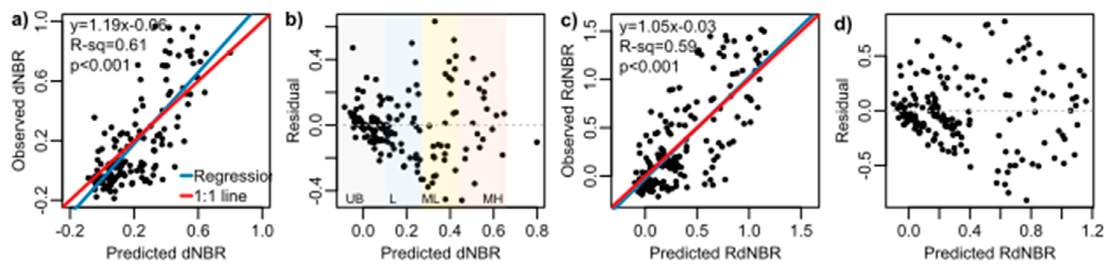
3.3. Fire Severity Prediction Based on Random Forest

dNBR values are correlated with burn severity, where high dNBR value suggests high fire severity. Random Forest regression was used to estimate dNBR. Figure 9a shows the regression result between predicted dNBR and observed dNBR using testing samples derived from Sentinel−2 forest map and burn map, where the linear relationship is significant with p < 0.001, R2 0.6072 and correlation coefficient 0.78. Another burn severity index relative differenced normalized burn ratio index (RdNBR) (=dNBR/sqrt(NBRpre-fire)) [39] was also employed in Random Forest to compare with dNBR. Linear relationship between predicted RdNBR (Figure 9c) and observed RdNBR is significant with p < 0.001, R2 0.5861. These results show the capability of using ATL08 metrics to estimate fire severity.
Figure 9b shows that variation of residuals is not constant, where the divergence of points increases with dNBR first and then decreases. In Figure 9d, divergence of points also increases and then decreases. Based on thresholds in Table 3, points in Figure 9b were classified into unburned (UB), low (L), moderate-low (ML) and moderate-high (MH) severity, where high severity was missing as only one point was over 0.66 in Figure 9b. Standard deviation of each class was calculated: UB 0.1034, L 0.1764, ML 0.3034, MH 0.2292, where points in moderate low severity got highest standard deviation which means highest uncertainty.

4. Discussion

4.1. Comparison of Sentinel−2 and Landsat 8

In this study, 24 LiDAR metrics were utilized as predictors for burned ATL08 segments classification. The classification accuracy reached 83%, which shows the feasibility of using ATL08 data for burn area mapping. This study suggests that it is possible to employ spaceborne LiDAR data in fire disturbances monitoring.
Optical images were used to provide a reference burn map and landcover map in previous experiments. The images were collected with the same spectral bands, from Blue band to SWIR2 band (Table 2). Given their different spatial resolution, we wanted to investigate the effect of using Landsat 8 and Sentinel−2 images on ICESat−2 segments classification. Using a Sentinel−2 derived forest map and burn map, we got 592 forest segments (including burned forest and unburned forest) from two study sites. For Landsat 8 data, there were 744 forest segments in total. Therefore, Landsat 8 data introduced many false forest segments compared with Sentinel−2 data. This phenomenon can partly explain why Landsat 8 derived segments have slightly lower classification accuracy. In Table 4, user’s accuracy and producer’s accuracy of burned segments are 81.54% and 74.65% to Sentinel−2 derived testing samples, 79.79% and 68.81% to Landsat 8 derived samples. Overall accuracies of testing samples using Random Forest are 83.15% and 76.23% for Sentinel−2 derived segments and Landsat 8 derived ones, respectively. These results demonstrate that Landsat 8 derived segments have slightly lower classification accuracy than that of Sentinel−2 derived segments. However, the accuracy of these two datasets are comparable in fire mapping, 83.15% versus 76.23%.

4.2. Comparison of Classification Methods

From Table 4 and Table 5, Random Forest performs better than logistics regression in ATL08 segments classification. Random Forest classification produces higher overall accuracy and kappa than that of logistic regression. Moreover, the user’s and producer’s accuracy of burned segments are also higher in Random Forest. Therefore, it can be seen that with the same training samples and testing samples, Random Forest can get better classification results. These benefits can be attributed to the capability of data processing without statistical assumptions (e.g., parametric). However, Random Forest is a black box model, which means users do not have access to a model.
In logistic regression, the stepwise procedure removes those insignificant metrics and helps to simplify the model. Although the accuracy of logistic regression is a little bit lower, it is more efficient in practice to have a simple model with acceptable accuracy.

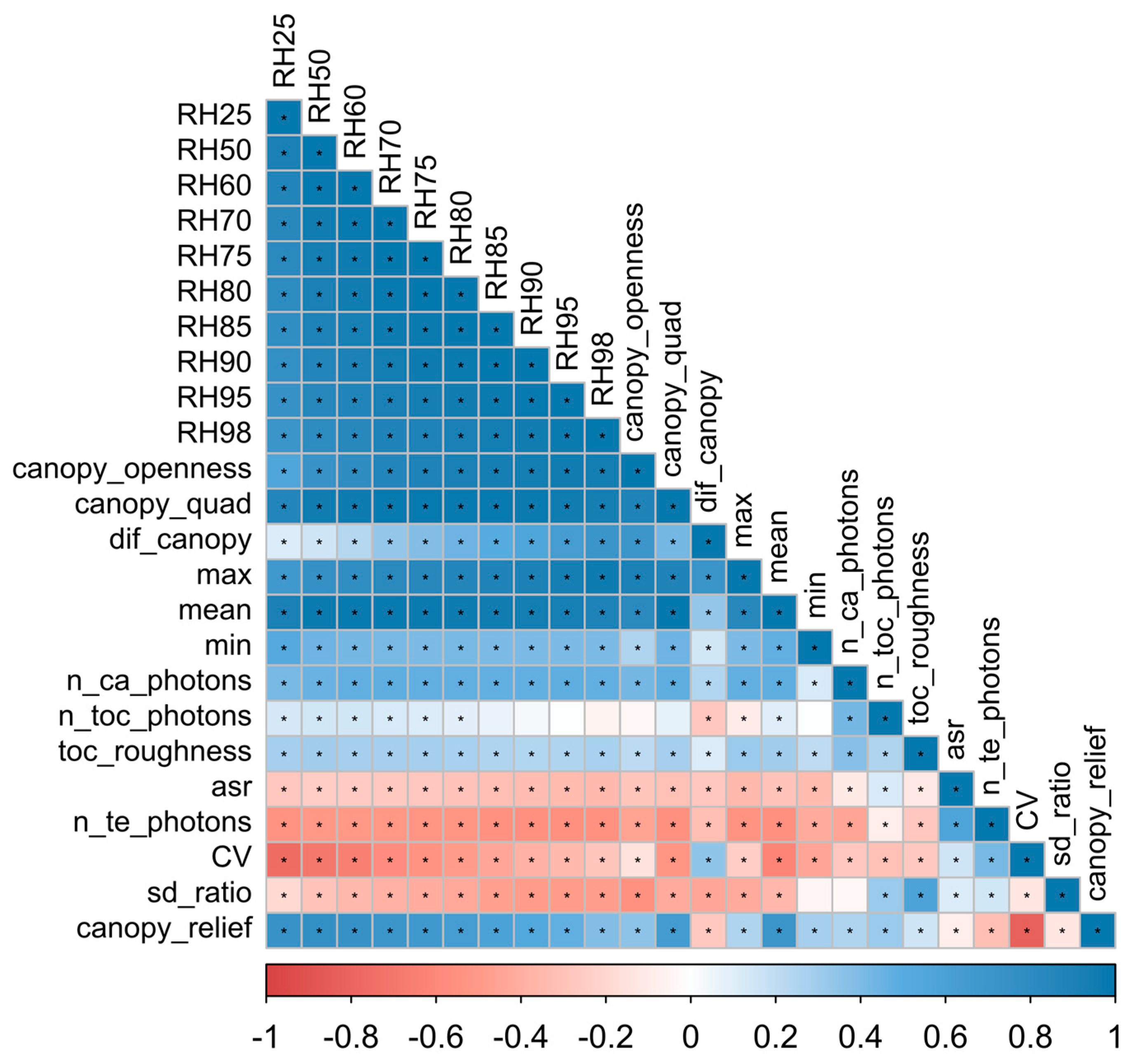
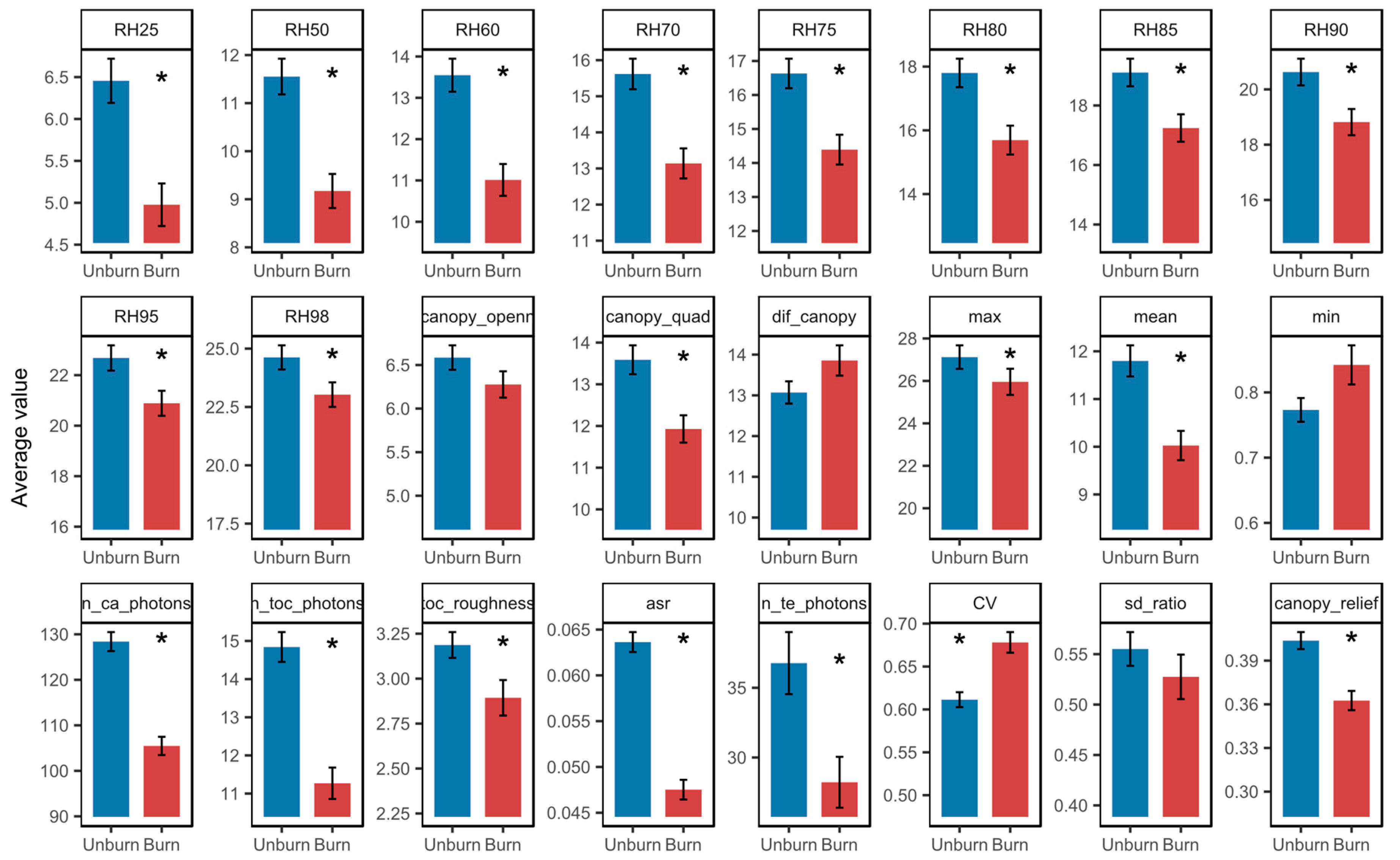
4.3. Comparison of LiDAR Metrics

Based on Figure 8, asr (apparent surface reflectance) is the most important metric (15.65% and 24.25% in importance) in burned ATL08 segments classification, n_ca_photons (the number of canopy photons) ranking the second. Other metrics such as n_te_photons (the number of terrain photons), n_toc_photons (the number of top of canopy photons), toc_roughness (top of canopy roughness), RH60, canopy_relief (canopy relief ratio) and CV (coefficient of variation) are less important. It is reasonable that reflectance contributes to capturing vegetation characteristics and changes. In Zhao et al. [40], intensity related metrics in airborne LiDAR explained 60% of variations in leaf area index, which also illustrates the importance of reflectance.
Other 23 LiDAR metrics count 84.35% and 75.57% in importance for Sentinel−2 based samples and Landsat 8 based samples, indicating the effectiveness of LiDAR data. To check the feasibility of using other LiDAR metrics in burn area classification, we removed asr and used the remaining 23 metrics to classify burned ATL08 segments, with 100% of the segments samples derived from Sentinel−2 data. Table 6 shows the OOB error (22.80%) that is acceptable without asr.
In fact, reflectance of optical images (asr in ATL08) is the sum of reflected photons within a pixel from which we cannot get height information directly. However, LiDAR helps to record the height information of each photons and based on which photons are classified into canopy photons and ground photons in ATL08, producing n_ca_photons and n_te_photons. Other metrics such as toc_roughness, RH60, canopy_relief and CV are also characteristics describing the 3D canopy structure which contribute to wildfire classification.

4.4. Limitations

The high classification accuracy shown in Table 4 reveals the feasibility of using ATL08 metrics for burned areas mapping along tracks. However, there are some limitations. First, it is unavoidable that there is time lag between the fire occurrence and acquisition of ICESat−2 data. We know the revisit time of ICESat−2 is 91 days currently. Therefore, the time lag between fire occurrence and ICESat−2 track will be around three months or two months. During the time lag, regrowth of forests after fire will reduce the difference between burned and unburned forests, causing more challenges in burned areas classification.
Moreover, logging or harvesting after fire will introduce damages to forest structure. This kind of change will cause interferences to fire mapping. At first, logging will produce debris and abandoned stems which might increase surface fuels. Second, large boles are removed and the density of canopy declines. Under this situation, data collected from ATL08 cannot represent structure changes in real fire events. However, our model still works as logging decreases canopy density and canopy height.
Moreover, the laser wavelength of the ICESat−2 ATLAS sensor is 532 nm, which makes it possible to be obstructed by clouds. In this case, no photons, or only very few photons, can reach the land surface when there are clouds. Therefore, only a small portion of the ICESat−2 data is suitable for land surface monitoring in the presence of clouds.

5. Conclusions

This study aims to investigate the feasibility of using ICESat−2 ATL08 data product to classify burned areas in wildfires. Both Sentinel−2 images and Landsat 8 data were used to produce reference land cover maps and burned maps. Twenty-four canopy related metrics derived from ATL08 were employed to classify burned segments with Random Forest and logistic regression, respectively. Our results indicate high classification accuracy of burned ATL08 segments based on both Sentinel−2 derived samples and Landsat 8 derived samples. Random Forest produced slightly higher classification accuracy than logistic regression. The number of canopy photons and apparent surface reflectance turned out to be the two most important metrics in classification. Metrics such as RH50, the number of top of canopy photons, coefficient of variation and canopy relief ratio are also helpful. It is anticipated that canopy related metrics will be more beneficial when differentiating fire severity as they characterize structure changes. This study demonstrates the feasibility of employing ATL08 for burned area mapping. As more ICESat−2 data accumulates over burned and unburned vegetation, and our understanding of photons description of canopy structure and ICESat−2 products such as ATL08 improve, we would expect to see more applications of using such data for assessing burned vegetation, fire severity and fuel loads. Future studies could also make use of a synergistic approach using ICESat−2 data and observations from other NASA missions, such as Global Ecosystem Dynamics Investigation (GEDI) and National Aeronautics and Space Administration-Indian Space Research Organization Synthetic Aperture Radar mission (NISAR), to improve the classification of burned and unburned areas and assess fire risk.

Supplementary Materials

The following are available online at https://www.mdpi.com/2072-4292/12/1/24/s1, Figure S1: Scatterplot of asr (apparent surface reflectance) to probabilities calculated by logistic regression models using testing samples from Sentinel-2 derived samples and Landsat 8 derived samples, respectively., Table S1: Confusion matrix of forest map classification based on Sentinel-2 data and Landsat 8 data in two study areas, where R_sum means row sum, C_sum is column sum, U_Acc is user’s accuracy and P_Acc is producer’s accuracy. Table S2: Confusion matrix of burn maps based on Sentinel-2 data and Landsat 8 data in two study areas. Table S3: Coefficients and 95% confidence intervals of logistic regression based on Sentinel-2 based samples and Landsat 8 based samples. VIF means variance of inflation factors.

Author Contributions

Method, experiments and writing original draft, M.L.; Funding source, ideas and manuscript revision, S.P.; Helping with data processing and manuscript revision, L.M. All authors have read and agreed to the published version of the manuscript.

Funding

This research was funded by NASA’s ICESat−2 SDT (Grant # NNX15 AD02 G). The open access publishing fees for this article have been covered by the Texas A&M University Open Access to Knowledge Fund (OAKFund), supported by the University Libraries and the Office of the Vice President for Research.

Acknowledgments

We would like to thank Texas A&M for providing study opportunities and publishing fees. Moreover, we appreciate PhD student Linqing Yang in Department of Ecosystem Science and Management in Texas A&M for providing help in plotting and data processing.

Conflicts of Interest

The authors declare no conflict of interest.

References

  1. Jolly, W.M.; Cochrane, M.A.; Freeborn, P.H.; Holden, Z.A.; Brown, T.J.; Williamson, G.J.; Bowman, D.M.J.S. Climate-induced variations in global wildfire danger from 1979 to 2013. Nat. Commun. 2015, 6, 7537. [Google Scholar] [CrossRef]
  2. Schoennagel, T.; Balch, J.K.; Brenkert-Smith, H.; Dennison, P.E.; Harvey, B.J.; Krawchuk, M.A.; Mietkiewicz, N.; Morgan, P.; Moritz, M.A.; Rasker, R.; et al. Adapt to more wildfire in western North American forests as climate changes. Proc. Natl. Acad. Sci. USA 2017, 114, 4582–4590. [Google Scholar] [CrossRef] [Green Version]
  3. Yue, C.; Ciais, P.; Cadule, P.; Thonicke, K.; van Leeuwen, T.T. Modelling the role of fires in the terrestrial carbon balance by incorporating SPITFIRE into the global vegetation model ORCHIDEE—Part 2: Carbon emissions and the role of fires in the global carbon balance. Geosci. Model Dev. 2015, 8, 1321–1338. [Google Scholar] [CrossRef] [Green Version]
  4. Chuvieco, E.; Mouillot, F.; van der Werf, G.R.; San Miguel, J.; Tanase, M.; Koutsias, N.; García, M.; Yebra, M.; Padilla, M.; Gitas, I.; et al. Historical background and current developments for mapping burned area 0from satellite Earth observation. Remote Sens. Environ. 2019, 225, 45–64. [Google Scholar] [CrossRef]
  5. Malambo, L.; Heatwole, C.D. Automated training sample definition for seasonal burned area mapping. ISPRS J. Photogramm. Remote Sens. In press.
  6. Pleniou, M.; Koutsias, N. Sensitivity of spectral reflectance values to different burn and vegetation ratios: A multi-scale approach applied in a fire affected area. ISPRS J. Photogramm. Remote Sens. 2013, 79, 199–210. [Google Scholar] [CrossRef]
  7. Koutsias, N.; Karteris, M. Burned area mapping using logistic regression modeling of a single post-fire Landsat-5 Thematic Mapper image. Int. J. Remote Sens. 2000, 21, 673–687. [Google Scholar] [CrossRef]
  8. Dragozi, E.; Gitas, I.Z.; Stavrakoudis, D.G.; Theocharis, J.B. Burned Area Mapping Using Support Vector Machines and the FuzCoC Feature Selection Method on VHR IKONOS Imagery. Remote Sens. 2014, 6, 12005–12036. [Google Scholar] [CrossRef] [Green Version]
  9. Escuin, S.; Navarro, R.; Fernández, P. Fire severity assessment by using NBR (Normalized Burn Ratio) and NDVI (Normalized Difference Vegetation Index) derived from LANDSAT TM/ETM images. Int. J. Remote Sens. 2008, 29, 1053–1073. [Google Scholar] [CrossRef]
  10. Fraser, R.H.; Van der Sluijs, J.; Hall, R.J. Calibrating Satellite-Based Indices of Burn Severity from UAV-Derived Metrics of a Burned Boreal Forest in NWT, Canada. Remote Sens. 2017, 9, 279. [Google Scholar] [CrossRef] [Green Version]
  11. Hawbaker, T.J.; Vanderhoof, M.K.; Beal, Y.-J.; Takacs, J.D.; Schmidt, G.L.; Falgout, J.T.; Williams, B.; Fairaux, N.M.; Caldwell, M.K.; Picotte, J.J.; et al. Mapping burned areas using dense time-series of Landsat data. Remote Sens. Environ. 2017, 198, 504–522. [Google Scholar] [CrossRef]
  12. Roteta, E.; Bastarrika, A.; Padilla, M.; Storm, T.; Chuvieco, E. Development of a Sentinel-2 burned area algorithm: Generation of a small fire database for sub-Saharan Africa. Remote Sens. Environ. 2019, 222, 1–17. [Google Scholar] [CrossRef]
  13. De Santis, A.; Chuvieco, E. GeoCBI: A modified version of the Composite Burn Index for the initial assessment of the short-term burn severity from remotely sensed data. Remote Sens. Environ. 2009, 113, 554–562. [Google Scholar] [CrossRef]
  14. Kato, A.; Moskal, L.M.; Batchelor, J.L.; Thau, D.; Hudak, A.T. Relationships between Satellite-Based Spectral Burned Ratios and Terrestrial Laser Scanning. Forests 2019, 10, 444. [Google Scholar] [CrossRef] [Green Version]
  15. Lefsky, M.A.; Cohen, W.B.; Harding, D.J.; Parker, G.G.; Acker, S.A.; Gower, S.T. Lidar remote sensing of above-ground biomass in three biomes. Glob. Ecol. Biogeogr. 2002, 11, 393–399. [Google Scholar] [CrossRef] [Green Version]
  16. Garcia, M.; Saatchi, S.; Casas, A.; Koltunov, A.; Ustin, S.; Ramirez, C.; Garcia-Gutierrez, J.; Balzter, H. Quantifying biomass consumption and carbon release from the California Rim fire by integrating airborne LiDAR and Landsat OLI data. J. Geophys. Res. Biogeosci. 2017, 122, 340–353. [Google Scholar] [CrossRef]
  17. Montealegre, A.L.; Lamelas, M.T.; Tanase, M.A.; de la Riva, J. Forest Fire Severity Assessment Using ALS Data in a Mediterranean Environment. Remote Sens. 2014, 6, 4240–4265. [Google Scholar] [CrossRef] [Green Version]
  18. Popescu, S.C. Estimating biomass of individual pine trees using airborne lidar. Biomass Bioenergy 2007, 31, 646–655. [Google Scholar] [CrossRef]
  19. Wang, C.; Glenn, N.F. Estimation of fire severity using pre- and post-fire LiDAR data in sagebrush steppe rangelands. Int. J. Wildland Fire 2009, 18, 848. [Google Scholar] [CrossRef] [Green Version]
  20. Narine, L.L.; Popescu, S.; Neuenschwander, A.; Zhou, T.; Srinivasan, S.; Harbeck, K. Estimating aboveground biomass and forest canopy cover with simulated ICESat-2 data. Remote Sens. Environ. 2019, 224, 1–11. [Google Scholar] [CrossRef]
  21. Popescu, S.C.; Zhou, T.; Nelson, R.; Neuenschwander, A.; Sheridan, R.; Narine, L.; Walsh, K.M. Photon counting LiDAR: An adaptive ground and canopy height retrieval algorithm for ICESat-2 data. Remote Sens. Environ. 2018, 208, 154–170. [Google Scholar] [CrossRef]
  22. Zwally, H.J.; Schutz, B.; Abdalati, W.; Abshire, J.; Bentley, C.; Brenner, A.; Bufton, J.; Dezio, J.; Hancock, D.; Harding, D.; et al. ICESat’s laser measurements of polar ice, atmosphere, ocean, and land. J. Geodyn. 2002, 34, 405–445. [Google Scholar] [CrossRef] [Green Version]
  23. Lefsky, M.A. A global forest canopy height map from the Moderate Resolution Imaging Spectroradiometer and the Geoscience Laser Altimeter System. Geophys. Res. Lett. 2010, 37. [Google Scholar] [CrossRef] [Green Version]
  24. Goetz, S.J.; Sun, M.; Baccini, A.; Beck, P.S.A. Synergistic use of spaceborne lidar and optical imagery for assessing forest disturbance: An Alaska case study. J. Geophys. Res. Biogeosci. 2010, 115, doi. [Google Scholar] [CrossRef] [Green Version]
  25. García, M.; Popescu, S.; Riaño, D.; Zhao, K.; Neuenschwander, A.; Agca, M.; Chuvieco, E. Characterization of canopy fuels using ICESat/GLAS data. Remote Sens. Environ. 2012, 123, 81–89. [Google Scholar] [CrossRef]
  26. Markus, T.; Neumann, T.; Martino, A.; Abdalati, W.; Brunt, K.; Csatho, B.; Farrell, S.; Fricker, H.; Gardner, A.; Harding, D.; et al. The Ice, Cloud, and land Elevation Satellite-2 (ICESat-2): Science requirements, concept, and implementation. Remote Sens. Environ. 2017, 190, 260–273. [Google Scholar] [CrossRef]
  27. Belgiu, M.; Drăguţ, L. Random forest in remote sensing: A review of applications and future directions. ISPRS J. Photogramm. Remote Sens. 2016, 114, 24–31. [Google Scholar] [CrossRef]
  28. Liu, T.; Abd-Elrahman, A.; Morton, J.; Wilhelm, V.L. Comparing fully convolutional networks, random forest, support vector machine, and patch-based deep convolutional neural networks for object-based wetland mapping using images from small unmanned aircraft system. GISci. Remote Sens. 2018, 55, 243–264. [Google Scholar] [CrossRef]
  29. Maxwell, A.E.; Warner, T.A.; Fang, F. Implementation of machine-learning classification in remote sensing: An applied review. Int. J. Remote Sens. 2018, 39, 2784–2817. [Google Scholar] [CrossRef] [Green Version]
  30. Breiman, L. Random Forests. Mach. Learn. 2001, 45, 5–32. [Google Scholar] [CrossRef] [Green Version]
  31. Wu, L.; Zhu, X.; Lawes, R.; Dunkerley, D.; Zhang, H. Comparison of machine learning algorithms for classification of LiDAR points for characterization of canola canopy structure. Int. J. Remote Sens. 2019, 40, 5973–5991. [Google Scholar] [CrossRef]
  32. Krishna Moorthy, S.M.; Bao, Y.; Calders, K.; Schnitzer, S.A.; Verbeeck, H. Semi-automatic extraction of liana stems from terrestrial LiDAR point clouds of tropical rainforests. ISPRS J. Photogramm. Remote Sens. 2019, 154, 114–126. [Google Scholar] [CrossRef] [PubMed]
  33. Neuenschwander, A.; Pitts, K. The ATL08 land and vegetation product for the ICESat-2 Mission. Remote Sens. Environ. 2019, 221, 247–259. [Google Scholar] [CrossRef]
  34. ATLAS/ICESat-2 L3A Land and Vegetation Height, Version 1 | National Snow and Ice Data Center. Available online: https://nsidc.org/data/ATL08/versions/1 (accessed on 12 September 2019).
  35. EarthExplorer—Home. Available online: https://earthexplorer.usgs.gov/ (accessed on 12 September 2019).
  36. Sen2Cor | STEP. Available online: https://step.esa.int/main/third-party-plugins-2/sen2cor/ (accessed on 12 September 2019).
  37. Otsu, N. A Threshold Selection Method from Gray-Level Histograms. IEEE Trans. Syst. Man Cybern. 1979, 9, 62–66. [Google Scholar] [CrossRef] [Green Version]
  38. The Normalized Burn Ratio. Available online: https://burnseverity.cr.usgs.gov/pdfs/lav4_br_cheatsheet.pdf (accessed on 6 December 2019).
  39. Miller, J.D.; Knapp, E.E.; Key, C.H.; Skinner, C.N.; Isbell, C.J.; Creasy, R.M.; Sherlock, J.W. Calibration and validation of the relative differenced Normalized Burn Ratio (RdNBR) to three measures of fire severity in the Sierra Nevada and Klamath Mountains, California, USA. Remote Sens. Environ. 2009, 113, 645–656. [Google Scholar] [CrossRef]
  40. Zhao, K.; Popescu, S. Lidar-based mapping of leaf area index and its use for validating GLOBCARBON satellite LAI product in a temperate forest of the southern USA. Remote Sens. Environ. 2009, 113, 1628–1645. [Google Scholar] [CrossRef]
Figure 1. Study area map, where the blue box on the upper left is northern California forest and the red box on the bottom is western New Mexico forest site.
Remotesensing 12 00024 g001
Figure 2. Satellite images visualized as false color composites (Near Infrared-Red-Green): (a) pre-fire Sentinel−2 image on July 12, 2018, (b) post-fire Sentinel−2 image on October 15, 2018, (c) pre-fire Landsat 8 image on July 10, 2018 and (d) post-fire Landsat 8 image on October 14, 2018 in northern California site; (e) pre-fire Sentinel−2 image on May 17, 2018, (f) post-fire Sentinel−2 image on June 21, 2018, (g) pre-fire Landsat 8 image on May 17, 2018 and (h) post-fire Landsat 8 image on June 27, 2018 in western New Mexico site. Burned areas tend to be black after fires.
Remotesensing 12 00024 g002
Figure 3. Flow chart of ATL08 segments classification procedures, where NDVI, NBR and dNBR are normalized difference vegetation index, normalized burn ratio index and differenced normalized burn ratio index.
Remotesensing 12 00024 g003
Figure 4. Classification maps: (a) Sentinel−2 forest map, (b) Sentinel−2 burn map, (c) Landsat 8 forest map, (d) Landsat 8 burn map in northern California site; (e) Sentinel−2 forest map, (f) Sentinel−2 burn map, (g) Landsat 8 forest map, (h) Landsat 8 burn map in western New Mexico site, where original ATL08 segments are labeled by the location of the center most photon and black polygons are fire perimeters. ATL08 data are discontinuous due to removal of segments with fill value.
Remotesensing 12 00024 g004
Figure 5. Correlations of 24 metrics from all ATL08 segments derived with Sentinel−2 forest maps and landcover maps in two study areas, where an asterisk (*) denotes significance, using Pearson test under 0.05 confidence level.
Remotesensing 12 00024 g005
Figure 6. Barplots of 24 metrics derived with Sentinel−2 data from both northern California and western New Mexico sties, where error bars are standard errors and an asterisk (*) denotes significance using Wilcoxon signed-rank test under 0.05 confidence interval. Blue bars mean unburned samples and red for burned samples.
Remotesensing 12 00024 g006
Figure 7. Random Forest classification of ATL08 forest segments (a) using Sentinel−2 derived samples and (b) Landsat 8 derived samples for northern California site; (c) using Sentinel−2 derived samples and (d) Landsat 8 derived samples for western New Mexico. Blue points are centermost photon of unburned segments and red for burned segments.
Remotesensing 12 00024 g007
Figure 8. Importance of each metric based on Mean Decrease of Gini index (provided by Random Forest) using (a) Sentinel−2 based samples and (b) Landsat 8 based samples, respectively. y axis means single Gini index over the sum of all Gini indices then multiply 100%.
Remotesensing 12 00024 g008
Figure 9. Relationship between (a) Random Forest predicted dNBR and observed dNBR; (b) residual to predicted dNBR; (c) predicted relative differenced normalized burn ratio index (RdNBR) to observed RdNBR; (d) residual to predicted RdNBR using testing samples derived from Sentinel−2 data. UB means unburned, L means low severity, ML means moderate low severity and MH means moderate high severity. Blue lines are regression lines and red lines are 1:1 lines.
Remotesensing 12 00024 g009
Table 1. Twenty-four canopy related Light detection and ranging (LiDAR) metrics, where the three bold ones are derived based on 21 metrics in ICESat-2 Land and Vegetation Height product (ATL08).
LabelGroupLong NameDescription
canopy_h_metrics: RH25, RH50, RH60, RH70, RH75, RH80, RH85, RH90, RH95, RH98gtx/land_segments/canopyCanopy height metricsHeight metrics based on the cumulative distribution of relative canopy heights above the interpolated ground surface. The height metrics are calculated at the following percentiles: 25,50,60,70,75,80,85,90,95, 98%
canopy_opennessgtx/land_segments/canopyCanopy opennessStandard Deviation of all photons classified as canopy photons within the segment to provide inference of canopy openness
h_canopy_quadgtx/land_segments/canopyCanopy quadratic meanThe quadratic mean height of individual classified relative canopy photon heights above the estimated terrain surface
h_dif_canopygtx/land_segments/canopyCanopy diff to median heightDifference between RH98 and RH50
h_max_canopygtx/land_segments/canopyMaximum canopy heightRelative maximum of individual canopy heights within segment
h_mean_canopygtx/land_segments/canopyMean canopy heightMean of individual relative canopy heights within segment
h_min_canopygtx/land_segments/canopyMinimum canopy heightThe minimum of relative individual canopy heights within segment
n_ca_photonsgtx/land_segments/canopyNumber of canopy photonsThe number of photons classified as canopy within the segment
n_toc_photonsgtx/land_segments/canopyNumber of top of canopy photonsThe number of photons classified as top of canopy within the segment
toc_roughnessgtx/land_segments/canopyTop of canopy roughnessStandard deviation of the relative heights of all photons classified as top of canopy within the segment
asrgtx/land_segmentsApparent surface reflectanceApparent surface reflectance of the 100 m segment
n_te_photonsgtx/land_segments/terrainNumber of ground photonsThe number of the photons classified as terrain within the segment
CV-Coefficient of variationcanopy_openness/h_mean_canopy
sd_ratio-Standard deviation ratiotoc_roughness/canopy_openness
canopy_relief-Canopy relief ratio(h_mean_canopy-h_min_canopy)/(h_max_canopy-h_min_canopy)
Table 2. Spectral bands of Sentinel−2 and Landsat 8 used in burn mapping, where unit of wavelength is µm.
Sentinel−2 BandsCenter WavelengthLower-UpperLandsat 8 BandsCenter WavelengthLower-Upper
-- 10.4430.435–0.451
20.4940.439–0.53520.4820.452–0.512
30.5600.537–0.58230.5610.533–0.590
40.6650.646–0.68540.6550.636–0.673
80.8340.767–0.90850.8650.851–0.879
111.6121.539–1.68161.6091.567–1.651
122.1942.072–2.31272.2012.107–2.294
Table 3. Burn severity based on dNBR from United States Geological Survey (USGS).
dNBR ValueSeverity Level
−0.5 ≤ dNBR < −0.25High Regrowth
−0.25 ≤ dNBR < −0.1Low Regrowth
−0.1 ≤ dNBR < 0.1Unburned
0.1 ≤ dNBR < 0.27Low
0.27 ≤ dNBR < 0.44Moderate-Low
0.44 ≤ dNBR < 0.66Moderate-High
0.66 ≤ dNBR < 1.33High
Table 4. Confusion matrix of testing data from Random Forest based on Sentinel−2 derived samples and Landsat 8 derived samples. The reference was based on visual interpretation.
Reference Reference
Sentinel−2 map UnburnBurnedR_SumU_AccLandsat 8 map UnburnBurnedR_SumU_Acc
Unburn951811384.07%Unburn953412973.64%
Burned12536581.54%Burned19759479.79%
C_Sum10771178 C_Sum114109223
P_Acc88.79%74.65% P_Acc83.33%68.81%
Table 5. Confusion matrix of testing data from logistic regression based on Sentinel−2 derived samples and Landsat 8 derived samples. The reference was based on visual interpretation.
Reference Reference
Sentinel−2 map UnburnBurnedR_SumU_AccLandsat 8 map UnburnBurnedR_SumU_Acc
Unburn852410977.98%Unburn833712069.17%
Burned22476968.12%Burned317210369.90%
C_Sum10771178 C_Sum114109223
P_Acc79.44%66.20% P_Acc72.81%66.06%
Table 6. Out of bag (OOB) error of Random Forest model by Sentinel−2 based ATL08 samples, with 100% of the samples for training.
Metrics for Random ForestTotal OOB ErrorOOB of UnburnedOOB of Burned
Use 24 metrics18.24%13.52%24.60%
Remove asr22.80%18.23%28.96%

