Detection and Delineation of Sorted Stone Circles in Antarctica


Abstract

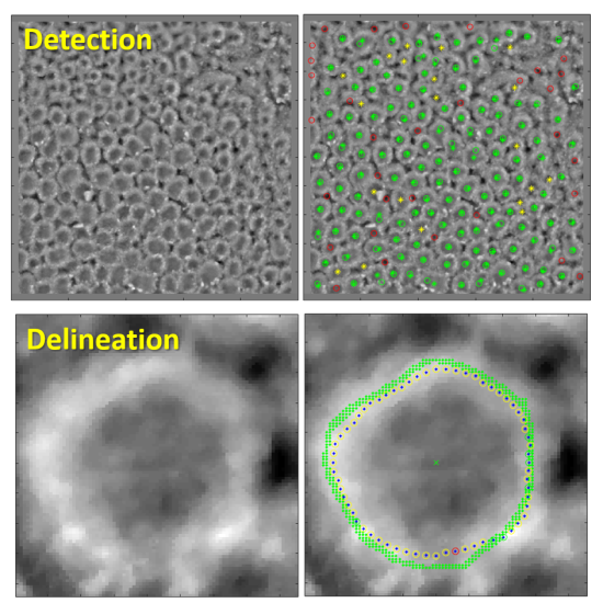
1. Introduction
- the delineation of the stone circle contour;
- an additional method based on dynamic programming;
- the evaluation of detection and delineation problems in an extended dataset.
2. Image Acquisition
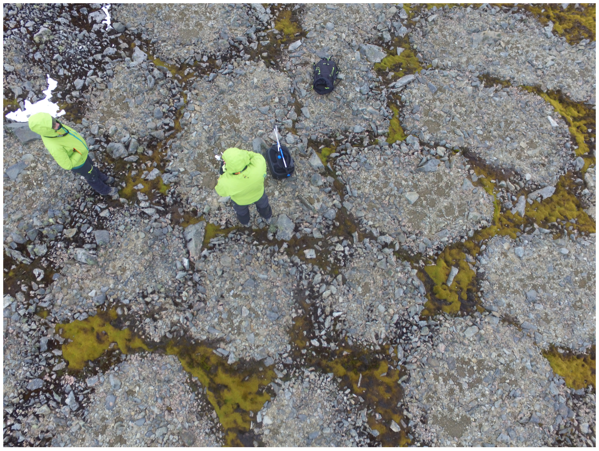
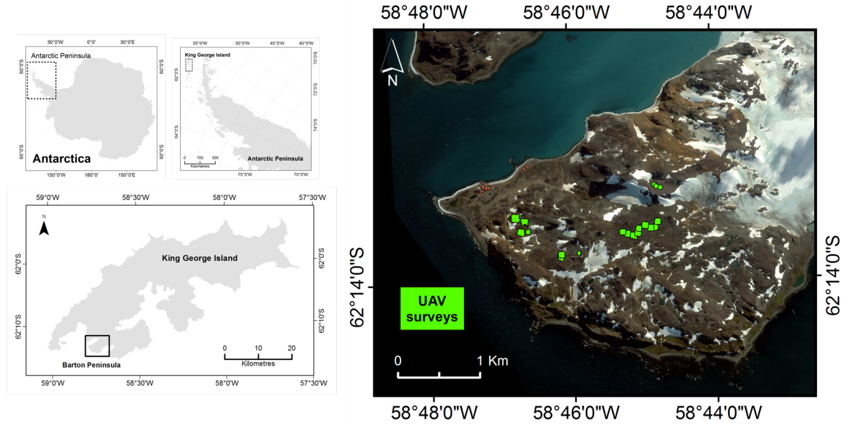
2.1. Study Area
2.2. UAV Surveys
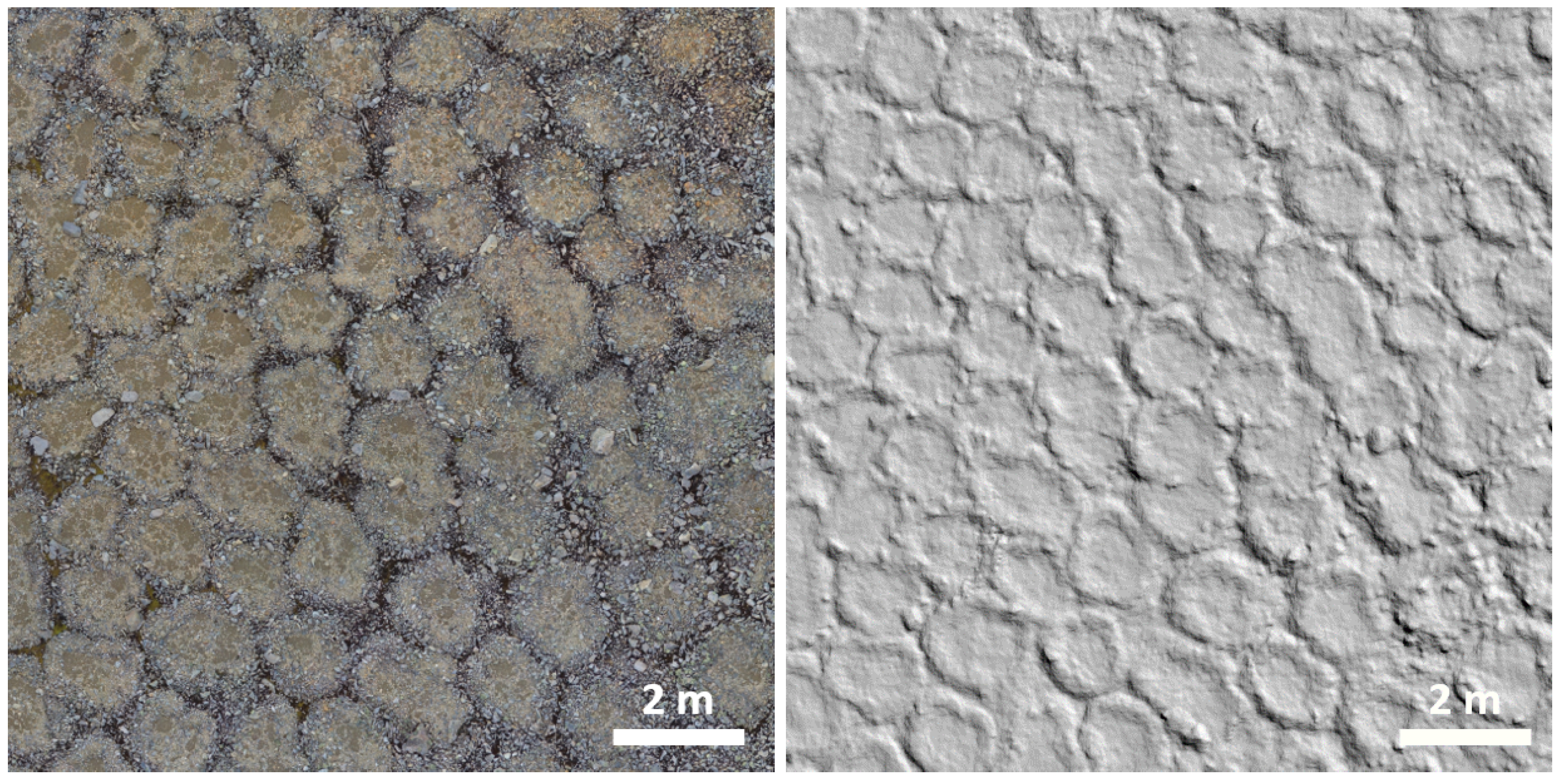
2.3. Mosaic and DEM Construction
3. Methods
3.1. Template Matching (TM)
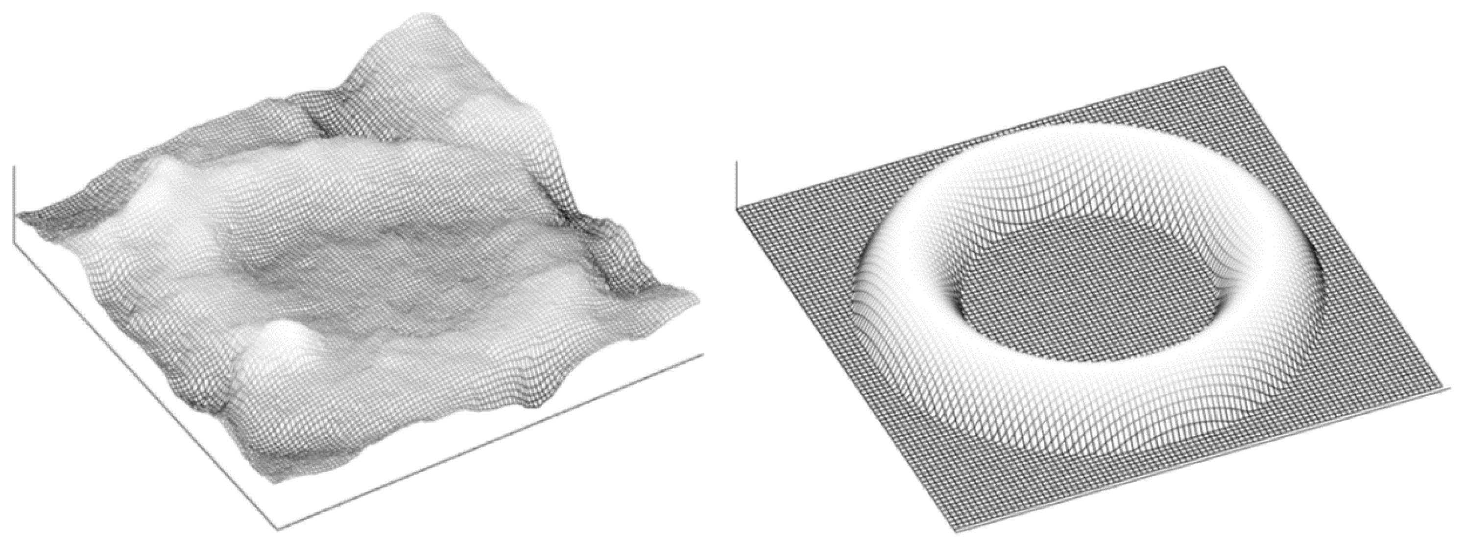
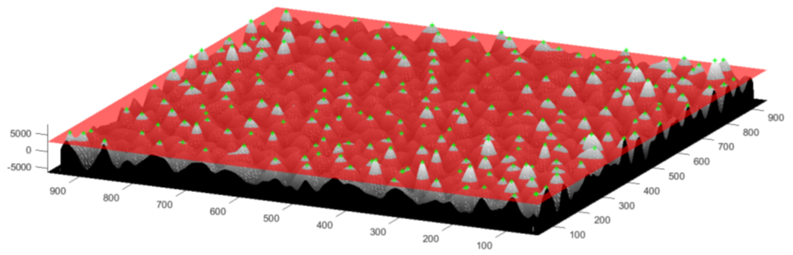
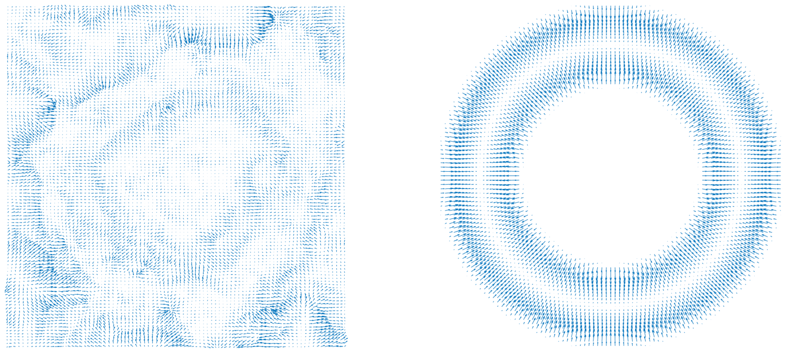
3.2. Sliding Band Filter (SBF)
3.3. Dynamic Programming (DP)
3.4. Contour Delineation
4. Results
4.1. Datasets
4.2. Performance Evaluation
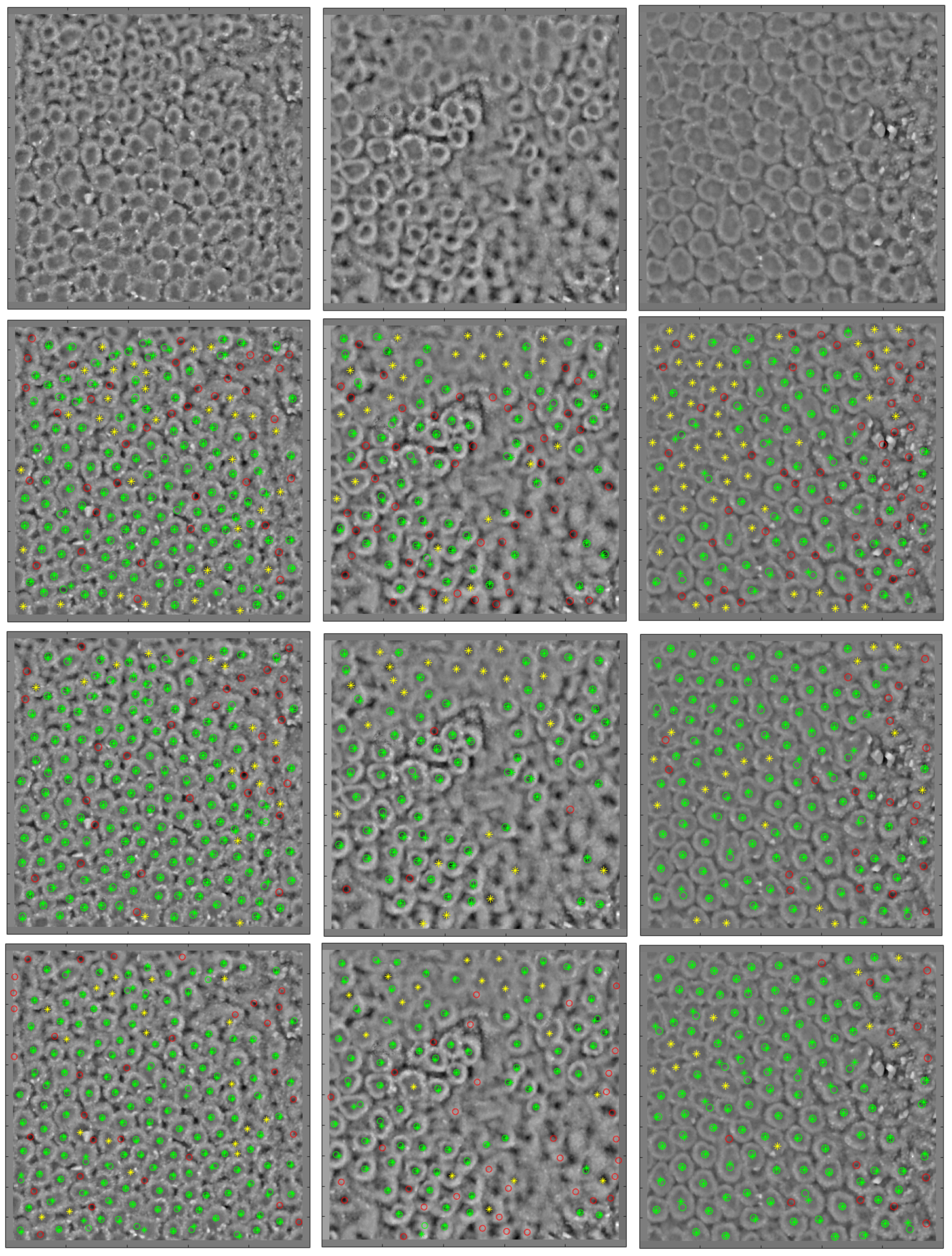
4.3. Detection
- TM: R = 30 pixels, = 0.4, = 35%.
- SBF: N = 128, = 80%.
- DP: N = 128, = 65%, = 1, m = 1.
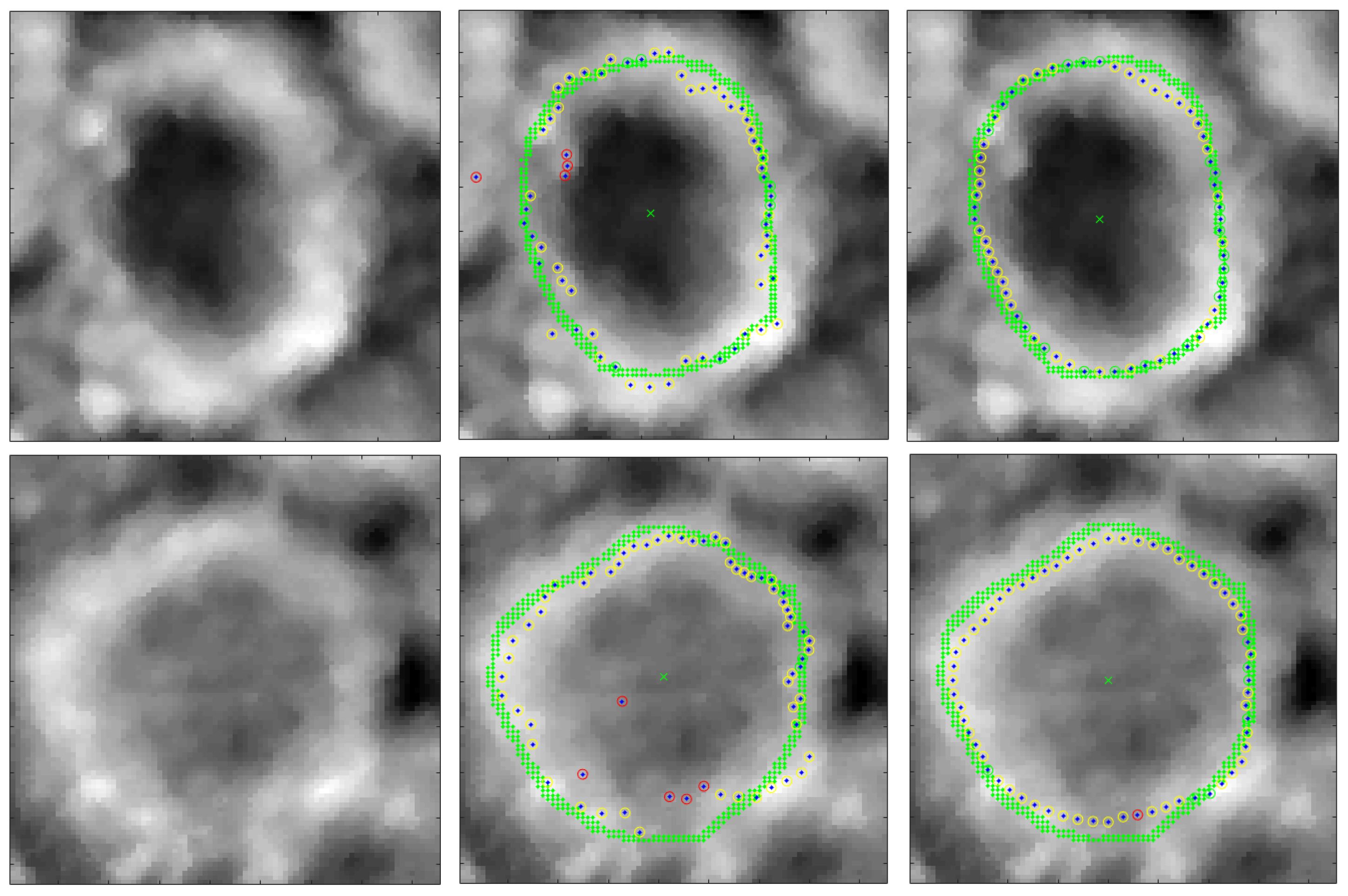
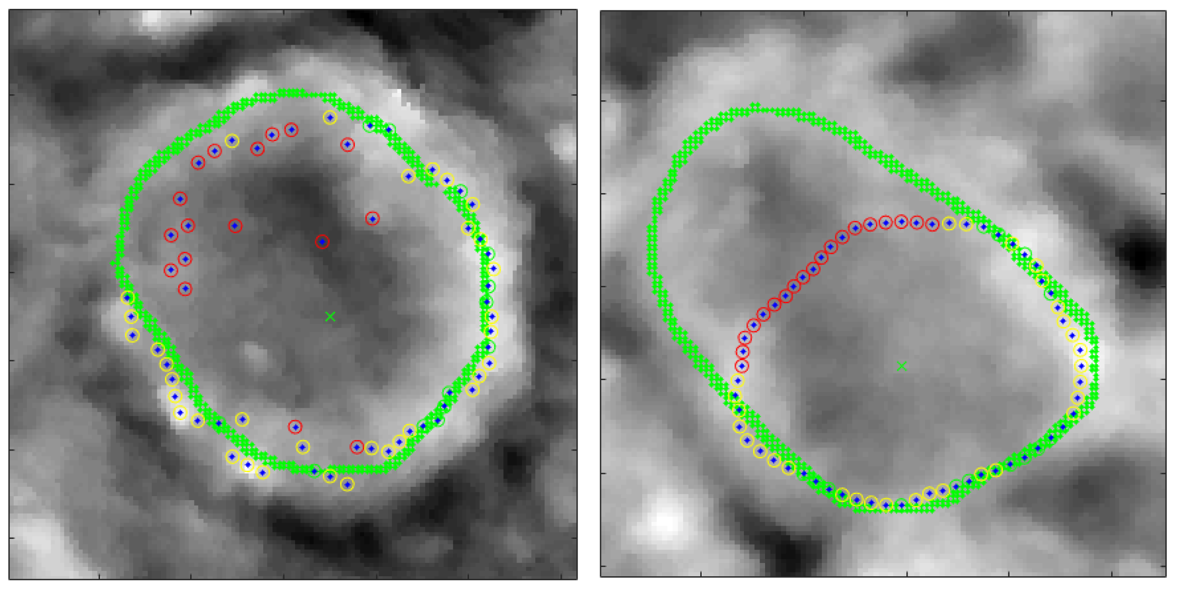
4.4. Delineation
5. Conclusions
Author Contributions
Funding
Acknowledgments
Conflicts of Interest
References
- Washburn, A.L. Geocryology: A Survey of Periglacial Processes and Environments; Wiley: New York, NY, USA, 1980. [Google Scholar]
- Hallet, B.; Prestrud, S. Dynamics of periglacial circles in Western Spitsbergen. Quat. Res. 1986, 26, 81–99. [Google Scholar] [CrossRef]
- Balme, M.R.; Gallagher, C.J.; Page, D.P.; Murray, J.B.; Muller, J.-P. Sorted stone circles in Elysium Planitia, Mars: Implications for recent martian climate. Icarus 2009, 200, 30–38. [Google Scholar] [CrossRef]
- Gallagher, C.; Balme, M.R.; Conway, S.J.; Grindrod, P.M. Sorted clastic stripes, lobes and associated gullies in high-latitude craters on Mars: Landforms indicative of very recent, polycyclic ground-ice thaw and liquid flows. Icarus 2011, 211, 458–471. [Google Scholar] [CrossRef]
- Hallet, B. Stone circles: Form and soil kinematics. Philos. Trans. R. Soc. A 2013, 371, 20120357. [Google Scholar] [CrossRef] [PubMed]
- Kaab, A.; Girod, L.; Berthling, I. Surface kinematics of periglacial sorted circles using structure-from-motion technology. Cryosphere 2014, 8, 1041–1056. [Google Scholar] [CrossRef]
- Kasprzak, M. High-resolution electrical resistivity tomography applied to patterned ground, Wedel Jarlsberg Land, south-west Spitsbergen. Polar Res. 2015, 34, 25678. [Google Scholar] [CrossRef]
- Slee, A.; Kiernan, K.; Shulmeister, J. Contemporary sorted patterned ground in low altitude areas of Tasmania. Geogr. Res. 2015, 53, 175–183. [Google Scholar] [CrossRef]
- Cox, G.W.; Allen, D.W. Sorted stone nets and circles of the Columbia Plateau: A hypothesis. Northwest Sci. 1987, 16, 179–185. [Google Scholar]
- Etzelmüller, B.; Sollid, J.L. The role of weathering and pedological processes for the development of sorted circles on Kvadehuksletta, Svalbard—A short report. Polar Res. 1991, 9, 181–191. [Google Scholar] [CrossRef]
- Jeong, G.Y. Radiocarbon ages of sorted circles on King George Island, South Shetland Islands, West Antarctica. Antarct. Sci. 2006, 18, 265–270. [Google Scholar] [CrossRef]
- Křížek, M.; Uxa, T. Morphology, sorting and microclimates of relict sorted polygons, Krkonoše Mountains, Czech Republic. Permafr. Periglac. Process. 2013, 24, 313–321. [Google Scholar] [CrossRef]
- Uxa, T.; Mida, P.; Křížek, M. Effect of climate on morphology and development of sorted circles and polygons. Permafr. Periglac. Process. 2017, 28, 663–674. [Google Scholar] [CrossRef]
- Kessler, M.A.; Murray, A.B.; Werner, B.T.; Hallet, B. A model for sorted circles as self-organized patterns. J. Geophys. Res. Solid Earth 2001, 106, 13287–13306. [Google Scholar] [CrossRef]
- Kessler, M.A.; Werner, B.T. Self-organization of sorted patterned ground. Science 2003, 299, 380–383. [Google Scholar] [CrossRef] [PubMed]
- Holness, S.D. Sorted circles in the Maritime Sub-Antarctic, Marion Island. Earth Surf. Process. Landforms 2003, 28, 337–347. [Google Scholar] [CrossRef]
- Haugland, J.E. Formation of patterned ground and fine-scale soil development within two late Holocene glacial chronosequences: Jotunheimen, Norway. Geomorphology 2004, 61, 287–301. [Google Scholar] [CrossRef]
- Yamagishi, C.; Matsuoka, N. Laboratory frost sorting by needle ice: A pilot experiment on the effects of stone size and extent of surface stone cover. Earth Surf. Process. Landforms 2015, 40, 502–511. [Google Scholar] [CrossRef]
- Pina, P.; Vieira, G.; Bandeira, L.; Mora, C. Accurate determination of surface reference data in digital photographs in ice-free surfaces of Maritime Antarctica. Sci. Total Environ. 2016, 573, 290–302. [Google Scholar] [CrossRef]
- Pudełko, R.; Angiel, P.J.; Potocki, M.; Jędrejek, A.; Kozak, M. Fluctuation of glacial retreat rates in the eastern part of Warszawa Icefield, King George Island, Antarctica, 1979–2018. Remote. Sens. 2018, 10, 892. [Google Scholar]
- Dabski, M.; Zmarz, A.; Pabjanek, P.; Korczak-Abshire, M.; Karsznia, I.; Chwedorzewska, K.J. UAV-based detection and spatial analyses of periglacial landforms on Demay Point (King George Island, South Shetland Islands, Antarctica). Geomorphology 2018, 290, 29–38. [Google Scholar] [CrossRef]
- Miranda, V.; Pina, P.; Heleno, S.; Vieira, G.; Mora, C.; Schaefer, C.E.G.R. Monitoring recent changes of vegetation in Fildes Peninsula (King George Island, Antarctica) through satellite imagery guided by UAV surveys. Sci. Total Environ. 2020, 704, 135295. [Google Scholar] [CrossRef] [PubMed]
- Turner, D.; Lucieer, A.; Malenovský, Z.; King, D.; Robinson, S.A. Assessment of Antarctic moss health from multi-sensor UAS imagery with random forest modelling. Int. J. Appl. Earth Obs. Geoinf. 2018, 68, 168–179. [Google Scholar] [CrossRef]
- Korczak-Abshire, M.; Zmarz, A.; Rodzewicz, M.; Kycko, M.; Karsznia, I.; Chwedorzewska, K.J. Study of fauna population changes on Penguin Island and Turret Point Oasis (King George Island, Antarctica) using an unmanned aerial vehicle. Polar Biol. 2019, 42, 217–224. [Google Scholar] [CrossRef]
- Pina, P.; Pereira, F.; Marques, J.S.; Heleno, S. Detection of stone circles in periglacial regions of Antarctica in UAV datasets. In Pattern Recognition and Image Analysis; Morales, A., Fierrez, J., Sánchez, J., Ribeiro, B., Eds.; Lecture Notes in Computer Science; Springer: Cham, Switzerland, 2019; Volume 11867, pp. 279–288. [Google Scholar]
- Yuen, H.K.; Princen, J.; Illingworth, J.; Kittler, J. Comparative study of Hough Transform methods for circle finding. Image Vis. Comput. 1990, 8, 71–77. [Google Scholar] [CrossRef]
- Mukhopadhyay, P.; Chaudhuri, B.B. A survey of Hough Transform. Pattern Recognit. 2015, 48, 993–1010. [Google Scholar] [CrossRef]
- Quelhas, P.; Marcuzzo, M.; Mendonça, A.M.; Campilho, A. Cell nuclei and cytoplasm joint segmentation using the sliding band filter. IEEE Trans. Med Imaging 2010, 29, 1463–1473. [Google Scholar] [CrossRef]
- Dias, J.M.B.; Leitão, J.M.N. Wall position and thickness estimation from sequences of echocardiographic images. IEEE Trans. Med Imaging 1996, 15, 25–38. [Google Scholar] [CrossRef]
- Marques, J.S.; Pina, P. Crater delineation by dynamic programming. IEEE Geosci. Remote. Sens. Lett. 2015, 12, 1581–1585. [Google Scholar] [CrossRef]
- Santiago, C.; Nascimento, J.C.; Marques, J.S. Fast segmentation of the left ventricle in cardiac MRI using dynamic programming. Comput. Methods Programs Biomed. 2018, 154, 9–23. [Google Scholar] [CrossRef]
- Oliva, M.; Antoniades, D.; Serrano, E.; Giralt, S.; Liu, E.J.; Granados, I.; Pla-Rabes, S.; Toro, M.; Hong, S.G.; Vieira, G. The deglaciation of Barton Peninsula (King George Island, South Shetland Islands, Antarctica) based on geomorphological evidence and lacustrine records. Polar Rec. 2019, 55, 177–188. [Google Scholar] [CrossRef]
- López-Martínez, J.; Serrano, E.; Schmid, T.; Mink, S.; Linés, C. Periglacial processes and landforms in the South Shetland Islands (northern Antarctic Peninsula region). Geomorphology 2012, 155–156, 62–79. [Google Scholar] [CrossRef]
- Smith, M.W.; Carrivick, J.L.; Quincey, D.J. Structure from motion photogrammetry in physical geography. Prog. Phys. Geogr. 2016, 40, 247–275. [Google Scholar] [CrossRef]
- Calviño-Cancela, M.; Martín-Herrero, J. Spectral discrimination of vegetation classes in ice-free areas of Antarctica. Remote. Sens. 2016, 8, 856. [Google Scholar] [CrossRef]
- Geiger, D.; Gupta, A.; Costa, L.A.; Vlontzos, J. Dynamic Programming for detecting, tracking, and matching deformable contours. IEEE Trans. Pattern Anal. Mach. Intell. 1995, 17, 294–302. [Google Scholar] [CrossRef]
- Amini, A.A.; Weymouth, T.E.; Jain, R.C. Using Dynamic Programming for solving variational problems in vision. IEEE Trans. Pattern Anal. Mach. Intell. 1990, 12, 855–867. [Google Scholar] [CrossRef]
- Marques, J.S.; Pina, P. An algorithm for the delineation of craters in very high resolution images of Mars surface. In Pattern Recognition and Image Analysis; Sanches, J.M., Micó, L., Cardoso, J.S., Eds.; Lecture Notes in Computer Science; Springer: Berlin/Heidelberg, Germany, 2013; Volume 7887, pp. 213–220. [Google Scholar]


| Forward Recursion | |
| Backward Recursion |
| Method | Parameters | Precision (%) | Recall (%) | F Score (%) | Time (min) |
|---|---|---|---|---|---|
| TM | R = 30, = 0.4, = 35 | 63.1 (11.7) | 72.7 (10.1) | 66.7 (8.9) | 0.1 (0.1) |
| SBF | N = 128, = 80 | 82.2 (14.5) | 84.2 (8.8) | 82.0 (6.6) | 14.9 (1.0) |
| N = 16, = 80 | 81.3 (14.4) | 83.9 (4.1) | 81.3 (6.9) | 1.8 (0.2) | |
| DP | N = 128, = 65, = 3, m = 1 | 85.2 (6.6) | 85.5 (14.8) | 85.2 (6.6) | 23.9 (12.9) |
| N=16, = 65, = 0.03, m = 1 | 87.0 (8.1) | 80.7 (8.4) | 84.3 (6.1) | 3.6 (1.6) |
| Method | Parameters | cp (%) | se (%) | ge (%) | Time (s) |
|---|---|---|---|---|---|
| SBF | N = 360 | 21.4 (9.4) | 60.4 (11.7) | 18.3 (18.8) | 5.5 (1.8) |
| N = 64 | 18.5 (8.5) | 63.5 (13.0) | 18.0 (18.8) | 4.4 (1.3) | |
| DP | N = 360, = 3 m = 1 | 27.6 (9.8) | 65.3 (10.6) | 7.1 (12.3) | 50.2 (14.3) |
| N = 64, = 0.3 m = 1 | 24.6 (10.3) | 68.2 (13.0) | 7.2 (13.7) | 3.2 (0.8) |
© 2020 by the authors. Licensee MDPI, Basel, Switzerland. This article is an open access article distributed under the terms and conditions of the Creative Commons Attribution (CC BY) license (http://creativecommons.org/licenses/by/4.0/).
Share and Cite
Pereira, F.; Marques, J.S.; Heleno, S.; Pina, P. Detection and Delineation of Sorted Stone Circles in Antarctica. Remote Sens. 2020, 12, 160. https://doi.org/10.3390/rs12010160
Pereira F, Marques JS, Heleno S, Pina P. Detection and Delineation of Sorted Stone Circles in Antarctica. Remote Sensing. 2020; 12(1):160. https://doi.org/10.3390/rs12010160
Chicago/Turabian StylePereira, Francisco, Jorge S. Marques, Sandra Heleno, and Pedro Pina. 2020. "Detection and Delineation of Sorted Stone Circles in Antarctica" Remote Sensing 12, no. 1: 160. https://doi.org/10.3390/rs12010160
APA StylePereira, F., Marques, J. S., Heleno, S., & Pina, P. (2020). Detection and Delineation of Sorted Stone Circles in Antarctica. Remote Sensing, 12(1), 160. https://doi.org/10.3390/rs12010160