Semi-Supervised Hyperspectral Image Classification via Spatial-Regulated Self-Training

Abstract

Because there are many unlabeled samples in hyperspectral images and the cost of manual labeling is high, this paper adopts semi-supervised learning method to make full use of many unlabeled samples. In addition, those hyperspectral images contain much spectral information and the convolutional neural networks have great ability in representation learning. This paper proposes a novel semi-supervised hyperspectral image classification framework which utilizes self-training to gradually assign highly confident pseudo labels to unlabeled samples by clustering and employs spatial constraints to regulate self-training process. Spatial constraints are introduced to exploit the spatial consistency within the image to correct and re-assign the mistakenly classified pseudo labels. Through the process of self-training, the sample points of high confidence are gradually increase, and they are added to the corresponding semantic classes, which makes semantic constraints gradually enhanced. At the same time, the increase in high confidence pseudo labels also contributes to regional consistency within hyperspectral images, which highlights the role of spatial constraints and improves the HSIc efficiency. Extensive experiments in HSIc demonstrate the effectiveness, robustness, and high accuracy of our approach.

1. Introduction

Due to the advance of optical sensing technology, hyperspectral images, which contain richer spectral information compared with Synthetic-Aperture Radar (SAR) and Red_Green_Blue (RGB) images, have attracted increasing attentions in the remote sensing field recently. To fully analyze raw hyperspectral images, hyperspectral image classification (HSIc) [1,2,3] plays a crucial role and is a prerequisite step towards many remote sensing applications [4,5], i.e., forest inventory, urban-area monitoring, resource exploration.

HSIc usually refers to the use of the spectral-spatial information of hyperspectral images to accurately map the spatial distribution and material content, and identify different types of features in the corresponding scene. But compared to the application of SAR or RGB images [6,7,8], there are two main challenges for HSIc: (1) redundancy of spectral information and (2) large datasets. In traditional methods, since the redundancy of spectral information about hyperspectral images, dimensionality reduction [9,10] is required to efficiently extract features. Chen et al. [11] applied Principal Component Analysis (PCA) [12,13] for dimension reduction to reduce redundant spectral features by linearly transposing raw high-dimensional data into a new low-dimensional data. Similarly, there are other ways to implement dimensionality reduction, such as Independent Component Analysis (ICA) [14], multivariate learning, or directly selecting the most representative channels from hyperspectral data. After that, low-dimensional data is obtained by preprocessing through the methods mentioned above, Stacked Autoencoder (SAE) [15] or Deep Belief Network (DBN) [16] have been introduced to classify objects (pixels) for low-dimensional data. However, in the process of dimensionality reduction, the original spectral structure may be destroyed, resulting in the loss of some useful spectral information, thus possibly reducing the performance of the HSIc.

In recent years, deep learning methods have caught the eyes from researchers as a tool of representation learning, and have made significant progress in computer vision [17], natural language processing [18], and speech recognition [19]. In the task of HSIc, deep learning methods also have became popular due to their impressive performance [20,21,22]. The features extracted by deep learning are better representation than hand-crafted features. Recently, spectral-spatial features extraction [23,24] methods based on convolutional neural networks (CNN) [25,26,27] have been proposed to make full use of spectral-spatial information by extracting the most discriminative regions and channels. Cao et al. [28] used the CNN classification results as the likelihood probability, and introduced the superpixel segmentation method as a prior one to regulate the final results. Yang et al. [29] used the migration learning to pre-train the CNN on other RGB-based remote sensing image datasets, and then fine-tune it on HSIc by end-to-end training. In all, the above methods can achieve promising performance in the HSIc on the condition that there are enough training samples.

Despite their great success, the deep learning methods heavily rely on enormous amounts of annotated data to achieve good results in supervised learning problems. However, labeling the data manually takes much time, which is a heavy burden for most researchers. Hyperspectral images are especially expensive and time-consuming to annotate as the knowledge and skill of experts are required which limits the power and application of deep learning models on hyperspectral images. For the above mentioned problems, the semi-supervised HSIc methods is proposed, which requires only a small number of labeled data.

In this paper, we introduce a novel semi-supervised HSIc framework relying on CNN for feature extraction and representation learning. The details of the proposed model could be composed of three steps: feature extraction, constrained clustering and spatial constraints. The following is the specific implementation process: first, the initial feature sets is extracted directly from the sample set, and each sample feature is a flattening of a certain size image patch centered on the sample. We implement a number of tiny-scale initial clusters with high self-consistency by over-clustering the initial feature sets. Next, a small number of initial labels are introduced as semantic constraints to assign pseudo labels to initial clusters, which makes these clusters merged into corresponding dominant semantic classes. The initial labels here are provided by the expert at the beginning and the pseudo labels are labels predicted by each iteration of the algorithm. To overcome erroneous pseudo labels, the spatial constraints are introduced to improve the HSIc accuracy under the smoothness assumption where neighboring pixels likely belong to similar classes. After clustering with semantic and spatial constraints, the pseudo labeles will increase. At the same time, the increase of highly confident pseudo labels also enrich the spatial neighborhood information, which enforces the role of spatial constraints. Finally, the pseudo labels are used for CNN training, and the trained network is used for features extraction. The features extracted by CNN will be more friendly to the next round of constraint clustering. This process loops until reaching the end condition.

In all, the contributions of this paper can be summarized as follows:

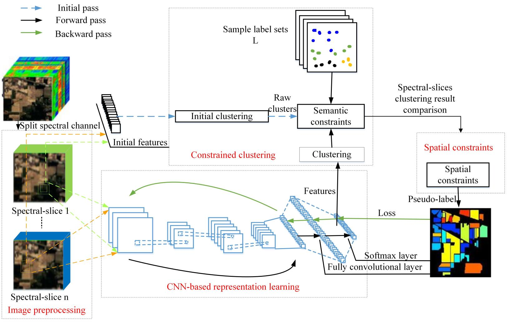
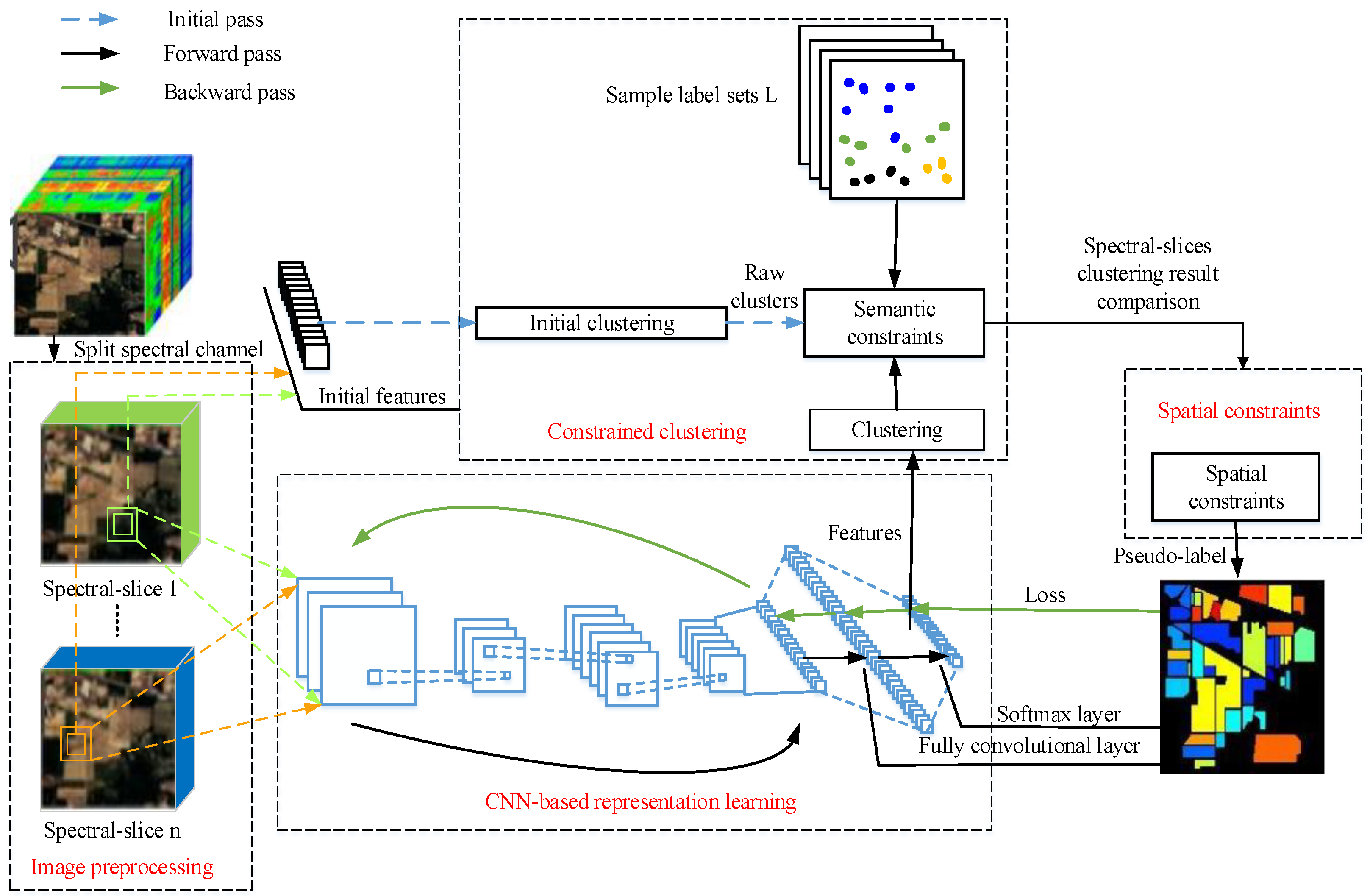
• We have introduced a novel semi-supervised classification algorithm for HSIc based on the cooperation between deep learning models and clustering.
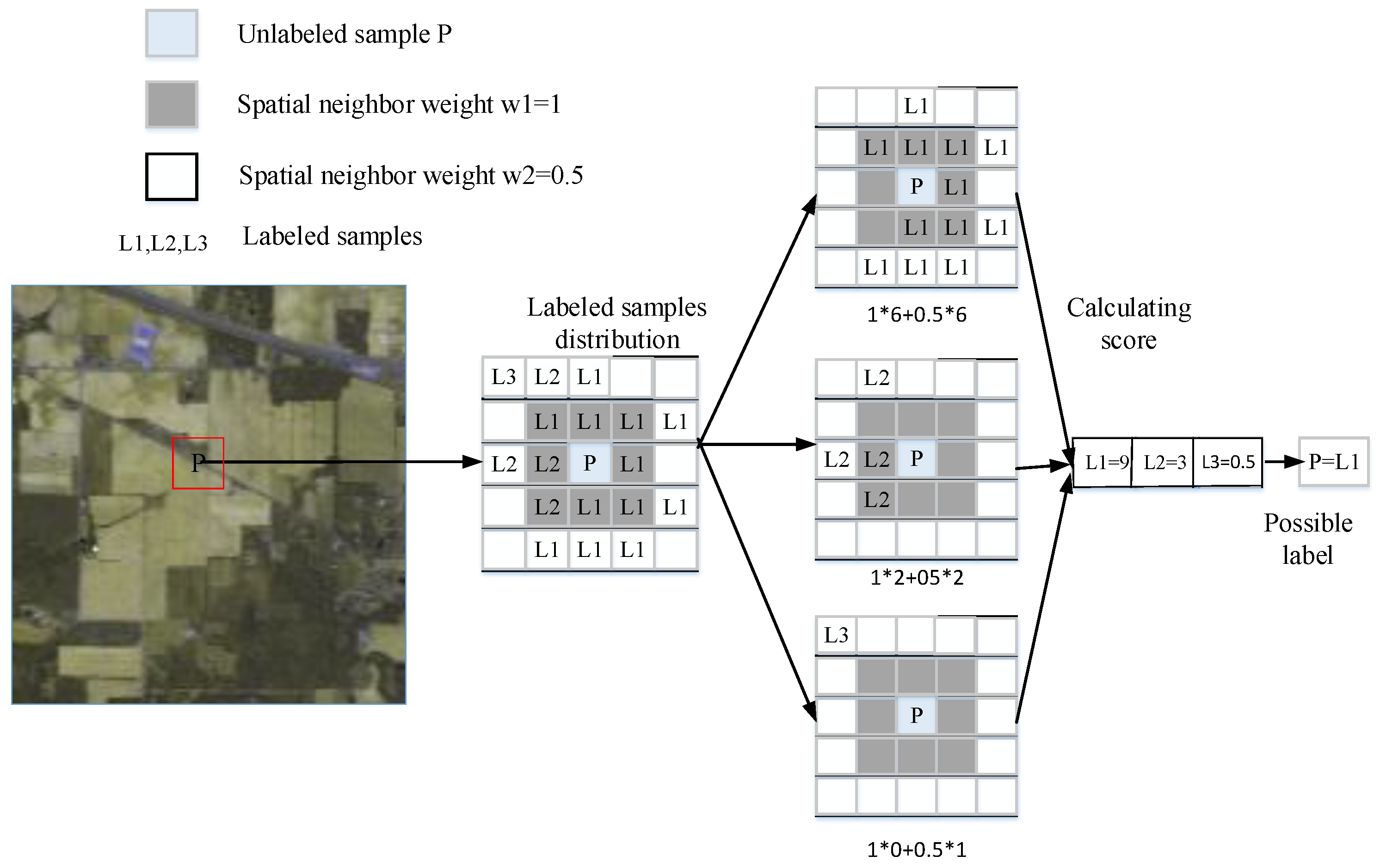
• Adjacent pixels in a hyperspectral image may belong to the same class. We introduce a spatial constraint in the above algorithm to give a smoothness hypothesis to improve HSIc accuracy.
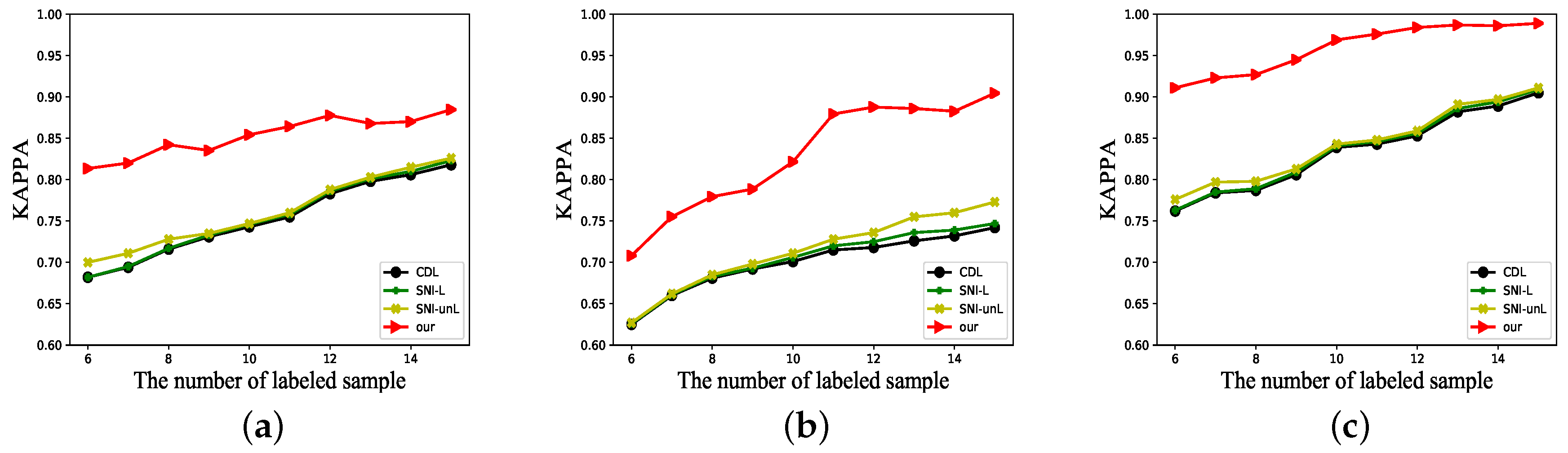
• Compared with previous methods, our proposed approach has achieved competitive performance on HSIc while leveraging tiny labeled data.

The remainder of this paper is organized as follows. Section 2 introduces relevant works. In Section 3, a HSIc framework is introduced. In Section 4, the corresponding experimental design and results are displayed. In Section 5, analysis and discussion of experiments. At last, the conclusions are summarized in Section 6.

2. Related Work

2.1. Hyperspectral Image Classification

We know that hyperspectral images contain two-dimensional spatial information and rich spectral information of the target scene. In hyperspectral images, each pixel corresponds to continuous spectral information of an object sample point, and every spectral channel includes location information of the target object. HSIc usually refers to the use of the spectral-spatial information of hyperspectral images to accurately map the spatial distribution and material content, and identify different types of features in the corresponding scene. In this paper, we use a semi-supervised learning approach to classify each pixel of the entire hyperspectral image by labeling a small number of labels for each scene, combined with a large number of unlabeled samples. The features of each pixel are the spectral-spatial features extracted by the CNN, making full use of the spectral-spatial information. HSIc is generally the first step to a variety of remote sensing applications including geological exploration [30], precision agriculture [31], and environmental monitoring [32], and it plays an important role in these areas.

In general, there are two methods for HSIc: pixel-wise methods and spectral–spatial methods. In the pixel-wise methods, the raw pixels with their labels are fed into the training models directly. In particular, SVM-based HSIc methods [33,34] have shown good performance, but they require a large number of labeled samples. In hyperspectral images, collecting annotated samples manually is very time-consuming and expensive, which makes this method limited.

In the spectral-spatial methods, both the marked and unmarked pixels are available for classification by using the neighborhood information of the labeled pixels. In hyperspectral images, spatially adjacent pixels typically have similar spectral features and tend to have similar classes [35]. As a result, spectral-spatial-based methods are more accurate [36]. Spectral-spatial methods are based on a variety of techniques, such as CNN [37,38], semi-supervised learning [39], Markov Random Field [40,41] and the ensembles of classifiers [42].

2.2. Semi-Supervised Learning

With the development of technology, the acquisition of hyperspectral image data becomes easy. However, obtaining labeled hyperspectral image data requires expert knowledge and it’s costly and time-consuming. Therefore, if only a small number of samples are labeled in the hyperspectral image data, cost will be saved. In HSIc applications, the commonly used supervised learning methods are limited by the number of labeled samples, and the semi-supervised learning methods can solve the problem of insufficient labeled samples. Semi-supervised learning has achieved good results in the classification of hyperspectral imagery. Ma et al. [43] proposed a feature learning algorithm, context deep learning (CDL), which is applied to HSIc. CDL uses a small number of training samples and a simple classifier to obtain high quality spectral and spatial features through a deep learning framework. Dópido et al. [44] proposed a semi-supervised classification method based on spatial neighbors with labeled samples (SNI-L) for HSIc, which adopts standard active learning methods into a self-learning scenarios, and uses machine-machine interaction instead of manual supervision to obtain new (unlabeled) samples. In order to utilize the rich information of hyperspectral images, Ma et al. [20] proposed a semi-supervised classification method based on multi-decision labeling and deep feature learning to achieve HSIc tasks. Tan et al. [45] proposed a semi-supervised HSIc method based on spatial neighborhood information of the selected unlabeled samples (SNI-unL), which combines the spatial neighborhood information of unlabeled samples with the classifier to improve the classification ability of selected unlabeled samples.

Many classical semi-supervised learning algorithms have been proposed. Commonly used generative methods are relatively easy to implement, and such methods assume that all samples (whether or not labeled) are “generated” by the same potential model. We can link unlabeled samples to learn objectives through the parameters of the potential model, while the unlabeled samples can be regarded as missing parameters of the model, and the maximum likelihood estimation can usually be solved based on the expectation-maximization (EM) [46] algorithm. But the algorithm has one key: the model hypothesis must be correct, otherwise using unlabeled data will reduce the generalization performance, which has great limitations in the real task. Transductive SVM (TSVM) [47] which maximize the spacing between different classes for all samples, but it’s difficult to deal with the problem having a large amount of unlabeled data. The graph-based [48] semi-supervised learning method is very clear in concept. It is easy to explore the nature of the algorithm by analyzing the matrix operations involved, but the algorithm also has great drawbacks: large storage overhead and sensitive to the structure of the graph. In this paper, we use an extension of the self-training algorithm [49] that is easy to implement. The method adds the high-confidence samples and the corresponding prediction labels to the pseudo labels in each iteration until all unlabeled samples have been added to the labels. The disadvantage of this method is that when the initial labels do not cover or represent the data space well, the initial training classifier will have a poor effect, which means a large number of misclassified samples will occur and remain. And the newly added misclassified labels in the subsequent iterations are the same. In our method, firstly, we use the method of repeating multiple experiments of randomly labeled subset to make the initial labels better cover the data space, and the initial classifier obtains better results. Secondly, we use semantic constraints and spatial constraints to make as few new misclassified labels as possible. Finally, the spectral-spatial features are extracted by CNN and applied to the classifier in the next episode.

3. Proposed Method

As illustrated in Figure 1, our method is a recurrent framework which consists of four modules: image preprocessing, CNN-based representation learning, constrained clustering and spatial constraints. A simple description of Figure 1: (1) Preprocessing of the image, the hyperspectral image is divided into $slice$ spectral-slices according to the number of spectral channels; (2) CNN (network structure based on LeNet [50] modification) performs spectral-spatial feature extraction for each spectral-slice separately; (3) The feature set extracted from each spectral-slice is separately constrained clustering to obtain the clustering results of all spectral-slices; (4) Similar to finding intersections between sets, the clustering results of each spectral-slice are compared. The results in each spectral-slice have the same semantic class as the HSIc result of the constrained clustering. (5) Adding a space constraint to the HSIc result to obtain a pseudo labels. (6) The generated pseudo labels and input data are input to the CNN for the next round of training. All the details are as follows.

Figure 1. Schematic of semi-supervised algorithm.

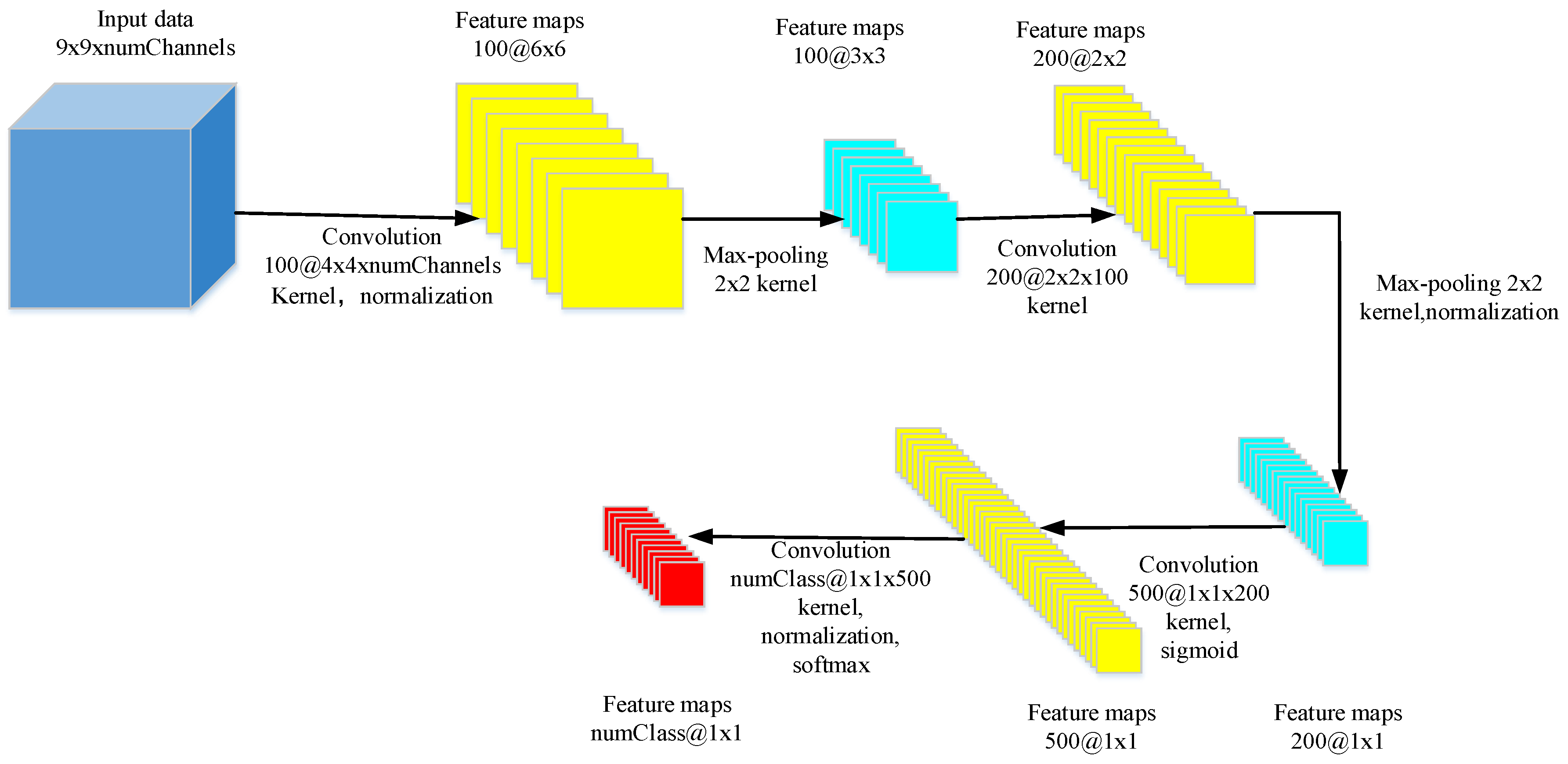
3.1. Feature Extraction Based on CNN Representation Learning

In order to take advantage of the spectral-spatial information of the hyperspectral image, we use CNN to extract spatial-spectral features. CNN can extract more representative features [51] compared to hand-crafted features, have strong feature learning capabilities and have been successful in image recognition.

Given a hyperspectral data set $P=(P_1,P_2,\dots ,P_N)$, N represents the total number of images, $P_n$ represents the n-th hyperspectral image. Each of these hyperspectral images are divided into $slice$ spectral-slices according to the number of spectral channels, and each of which contains $1/slice$ spectral channel of the original image. Then, the same operation is performed on all the spectral-slices: taking m small patches centered on each pixel, and each image has $m\times slice$ small patches. The size of the patches is $e\times e\times t$, where e is the width of the patches and t is the number of spectral channels of the patches. All the small patches of a spectral-slices of the n-th image can be represented as following:

$$\begin{array}{c}{Z}_n=\{z_{n,i}\in {\mathbb{R}}^U|i=1,2,\dots ,m\times slice;U=e\times e\times t\}\hfill \end{array}$$

(1)

where $Z_n\in Z$ and Z is defined as the full set of all the patches of the data set. As shown in Figure 1, $X_n$ denotes the features extracted from the CNN of the n-th image, where $X_n\in X$ and X is defined as the collection of extracted features of the full set. $X_n$ could be formulated as:

$$X_n=f(Z_n;\theta )$$

(2)

where $\theta$ denotes the parameters of CNN and f represents the forward pass function.

Network Structure

In this paper, our CNN structure is similar to LeNet, except that we abandon the full connected layer, change it to a full convolutional layer [52] and adjust the size and number of convolutional layer kernels. The network structure details are shown in Figure 2:

Figure 2. Network structure details.

3.2. Classification Processing

3.2.1. Constraints Based on Semantic Information

In this paper, we introduce a constrainted clustering scheme [53]. We perform the same operation on all spectral-slices of the hyperspectral image: taking m small patches centered on each pixel, and each spectral-slice has m small patches. $Z^n=(z_{n1};z_{n2};\dots ;z_{nm})$ is all small patche sets for the n-th spectral-slice. $X^n=(x_{n1};x_{n2};\dots ;x_{nm})$ denotes a feature vector set extracted from the CNN of the n-th spectral-slice. $X^n$ could be formulated as $X^n=f(Z^n;\theta )$. We separately over-clustered each spectral-sliced feature vector set. The feature vector set $X^n=(x_{n1};x_{n2};\dots ;x_{nm})$ is divided into k clusters $C=\{C_1,C_2,\dots ,C_k\}$ by K-means algorithm.

The over-clustering method yields many small clusters, and the samples in these clusters likely belong to one class. However, the image feature annotation needs to get the semantic information of the feature. So, we need to use a small amount of labeled information as the semantic constraint to identify the semantic information of each cluster. Clusters belonging to the same semantic constraint in clusters generated by over-clustering will be merged into the same semantic cluster.

No corresponding semantic labels and semantic information in the over-clustering clusters are classified into “unknown classes”. Since the labels in the semantic cluster are based on semantic distribution, the training pairs can make the neural network learn better feature representation. So in the next iteration, enlarging the over-clustering clusters can make the constrained clustering process more efficient. In the iterative optimization process, the number of over-clustering clusters decreases exponentially until the value is equal to the $K^{\ast }$. $K^{\ast }$ is generally set to double or triple the number of semantic objects contained in the image.

3.2.2. Sample Confidence Calculation

The calculation of sample confidence in the over-clustering process requires to know the label information. The initial over-clustering requires initial labels, and the subsequent over-clustering requires pseudo labels. The calculation process is as follows:

First, calculate the number of labels per cluster:

$$S_i={\displaystyle \sum _{q=1}^K}{\displaystyle \sum _{j=1}^{N_{p,i}}}pt(i,j,q),q\in \{0,1,\dots ,K\},j\in \{1,2,\dots ,N_{p,i}\}$$

(3)

Then, calculate the average number of labels per cluster:

$$S_{ave}=\frac{\sum S_i}{N_c}$$

(4)

where, K is the number of classes, $N_c$ is the number of clusters, $N_{p,i}$ is the number of samples included in the i cluster, $pt(i,j,q)$ indicates that the label of the j-th sample in the i-th cluster is q. When $q=0$, it means that the label is the background, and $pt(i,j,q)=0$, else $pt(i,j,q)=1$.

Secondly, the purity of the labels in the cluster is calculated, and the purity of the labels of the type f of the i cluster is:

$$PUR{E}_{i,f}=\frac{{\displaystyle \sum _{j=1}^{N_{p,i}}}pt(i,j,f)}{S_i},f\in \{1,2,\dots ,K\}$$

(5)

where $PUR{E}_{i,max}$ is the maximum value in the $PUR{E}_{i,f}$. When $PUR{E}_{i,max}$ is greater than the threshold $TH$ and $S_i>S_{ave}$. Currently, the cluster contains more labels and the number of samples belonged to category f is larger. Currently, we think that the cluster has a higher confidence which belongs to the f class. The value of $TH$ is usually set to 50% to 80% according to the specific situation.

Finally, we compare the clustering results of the $slice$ spectral-slices. Only the samples of the same semantic class in the clustering results of the $slice$ spectral-slices are used as the classification results of the over-clustering process.

3.2.3. Constraints Based on Neighborhood Spatial Information

In the previous introduction, we obtain the pseudo labels by clustering constraints. In this section, considering the fact that neighboring pixels in the hyperspectral image space domain likely belong to the same class, we introduce a local decision [20] strategy to smooth the pseudo labels. First, in the square neighborhood centered on the selected unlabeled sample, we count the labeled samples for a certain class with weight. Since the labels that near the test sample should have more decision power than the further appear label, the weight should relate to the two-dimensional Euclidean distance. Then sort the possible class scores. The label with the highest score is the final conclusion of the local decision. A simple example of a local decision process is as follows:

As shown in Figure 3, we assume that there are three types of labeled samples $L1$, $L2$, and $L3$ in the square field centered on the sample point P, and spaces indicate unlabeled samples. We count the three types of labeled samples with different weights. The formula for calculating the i-th score is as follows:

$$S_{L_i}=w1\times N_{L_i,1}+w2\times N_{L_i,2}$$

(6)

where $w1$ represents the weight of the 8 labeled samples around the first circle around the sample P, and $w2$ represents the weight of the 16 labeled samples adjacent to the second circle around the sample P. In this experiment we take $w1=1$ and $w2=0.5$. We sort the calculated label scores, and the highest score label is the final conclusion of the local decision.

Figure 3. Schematic based on the local neighborhood information constraint.

The class with the highest score is $L1$, and we set a threshold $ThreshHold$. The setting of $ThreshHold$ is related to the values of weights $w1$ and $w2$, and in this paper we take $ThreshHold=8$. When the score of $L1$ is greater than $Threshold$, we think that the higher confidence of sample point P belongs to category $L1$, otherwise it is not.

3.2.4. Iteration Process Based on Self-Training

As shown in Algorithm 1, the specific process is as follows: first, we divide the hyperspectral image into $slice$ spectral-slices according to the number of spectral channels. The number of spectral in the spectral-slice is $1/slice$ of the original image. In this paper we divide each hyperspectral image into four spectral-slices. Then, we extract the raw feature set $X^1$ = {X${}_1^0$, X${}_2^0$, ..., X${}_4^0$} from each of the four spectral-slices, and $X_4^1$ represents the feature set extracted from the 4th spectral-slice at the 1-th time, each feature from the flattening of the sample patch centered on the sample and has a size of $5\times 5$. Next, the initial labels L is introduced into the feature set of each spectral-slice, where L is a small number of labels obtained by repeating multiple experiments of randomly labeled subset, so that the initial labels can better cover the data space. And a separate over-clustering process is performed to obtain the raw cluster $K^0$ = {K${}_1^0$, K${}_2^0$, ..., K${}_4^0$}, and$K_n^1$ represents the clustering result of the 1-th constrained cluster of the 4th spectral-slice. Apply semantic constraints to $K^0$ by introducing L and comparing the clustering results of each spectral-slice, we will only use it as the clustering result $C^0$ for the samples that are assigned to the same semantic class. Finally, the initial classification result $Y^0$ is obtained by spatial constraint in the clustering result $C^0$.

In the subsequent training, the feature set $X^t$ = {X${}_1^t$, X${}_2^t$, ..., X${}_4^t$} is directly extracted from the fully convolutional layers of the CNN (t represents t iteration), and $X_4^t$ represents the feature set extracted from the 4th spectral-slice at the t-th time. Each feature comes from a sample-centric image patch of size $9\times 9$ which CNN encoded. Subsequent constrained clustering and spatial constraining processes are similar to the initial process, except updated each classification result $Y^t$ (t represents the t-th classification result). A new round of training is performed on the CNN with updated Y and input data. So iteratively, stop after satisfying the end condition. In this paper, we have found through many experiments that the HSIc accuracy tends to converge when iteration is about 12 rounds.

Algorithm 1 HSIc algorithm based on self-training

1: Input: 2: I = input hyperspectral image set. 3: L = initial label sets of hyperspectral images. 4: T = number of training epochs. 5: $K^{\ast }$ = number of over-clustering clusters. 6: Output: 7: $Y^{\ast }$ = final results of hyperspectral images classification. 8: $\theta {}^{\ast }$ = final parameters of CNN. 9: divide image set I into n spectral-slices set Z = $\{Z_1,Z_2,\dots ,Z_n\}$. 10: extract the initial feature set $X^1$ = {X${}_1^0$, X${}_2^0$, ..., X${}_n^0$} from each spectral-slice. 11: obtain the initial clustering results $K^0$ = {K${}_1^0$, K${}_2^0$, ..., K${}_n^0$} by K-means clustering. 12: apply semantic constraints to $K^0$ by introducing L and compare the initial clustering results of each spectral-slice to get $C^0$. 13: apply spatial constraints to $C^0$ to get the initial $Y^0$ 14: initialize parameters of CNN ${\theta }^1$. 15: $t\leftarrow 1$ 16: while$K^t>K^{\ast }$ or $t<T$ do 17:     update ${\theta }^t$ to ${\theta }^{t+1}$ by training CNN with labels $Y^t$. 18:     update $X^t$ to $X^{t+1}$ by feeding Z into CNN. 19:     obtain the clustering results $K^t$ by K-means clustering. 20:     apply semantic constraints to $K^t$ by introducing $Y^{t-1}$ and compare the clustering results of each spectral-slice to get $C^t$. 21:     apply spatial constraints to $C^t$ to get the $Y^t$ 22:     $t\leftarrow t+1$ 23: end while 24: return$Y^{\ast }\leftarrow Y^t$; ${\theta }^{\ast }\leftarrow {\theta }^t$;

In each iteration, the CNN is optimized by the BP (back propagation) algorithm [54].

4. Experimental Results

4.1. Data Sets

To assess the efficacy of our method, we use three publicly available hyperspectral data sets (http://www.ehu.eus/ccwintco/index.php?title=Hyperspectral_Remote_Sensing_Scenes): The first hyperspectral image used in experiments was collected by the $AVIRIS$ sensor over the Indian Pines region in Northwestern Indiana in 1992. And the second hyperspectral data set was collected by the $ROSIS$ optical sensor over the urban area of the University of Pavia, Italy. The third scene was collected by the 224-band $AVIRIS$ sensor over Salinas Valley, California. The detailed descriptions of these datasets are listed as follows.

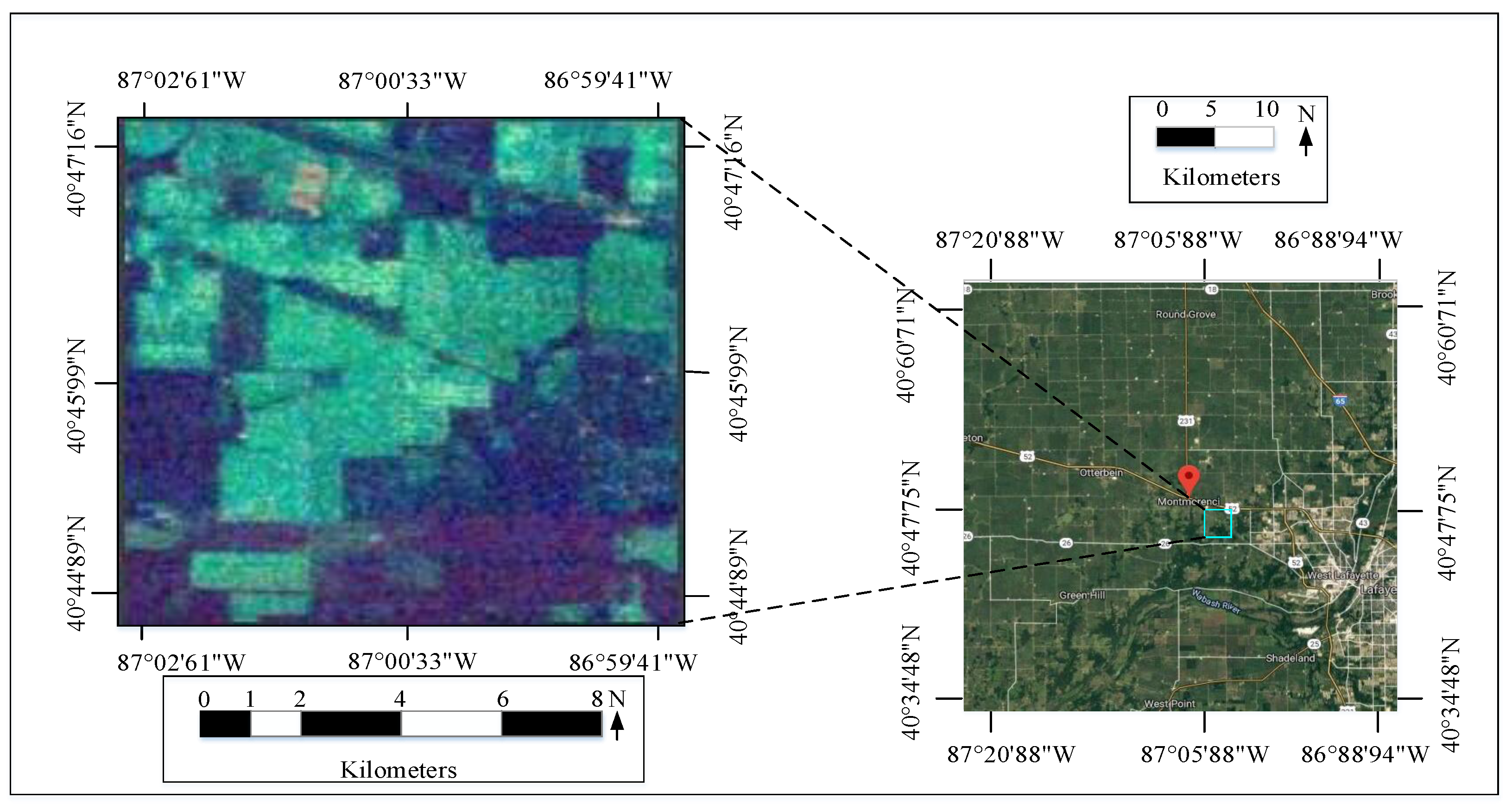
4.1.1. Indian Pines Data Set

The Indian Pines data set is shown in Figure 4. It consists of $145\times 145$ pixels and 224 spectral reflectance bands in the wavelength range 0.4–2.5 $\mathsf{\mu }$m. This scene contains two-thirds of agriculture and one-third of forests or other natural perennial vegetation. There are two main two-lane highways, one rail line, and some low-density housing, other building structures and smaller roads. Due to the emergence of some crops in June, corn and soybeans are in an early stage of growth with coverage below 5 percent. The available samples are divided into 16 categories for a total of 10,366 samples. The number of bands is reduced to 200 by removing the band covering the water absorption area. The actual sample categories and numbers and colors of this data set are as Table 1.

Figure 4. Indian Pines dataset: The left picture shows the pseudo-color of Indian Pines dataset, and the right picture shows the geographical location of Indian Pines dataset.

Table 1. Indian Pines Data Set.

Serial Number	Colour	Class	Sample Number	Serial Number	Colour	Class	Sample Number
1		Alfalfa	54	9		Oats	20
2		Corn-notill	1434	10		Soybean-notill	968
3		Corn-mintill	834	11		Soybean-mintill	2468
4		Corn	234	12		Soybean-clean	614
5		Grass/pasture	497	13		Wheat	212
6		Grass/tree	747	14		Woods	1294
7		Grass/pasture/mowed	26	15		Buildings/grass/trees/drives	95
8		Hay/windrowed	489	16		Stone/steel/towers	380

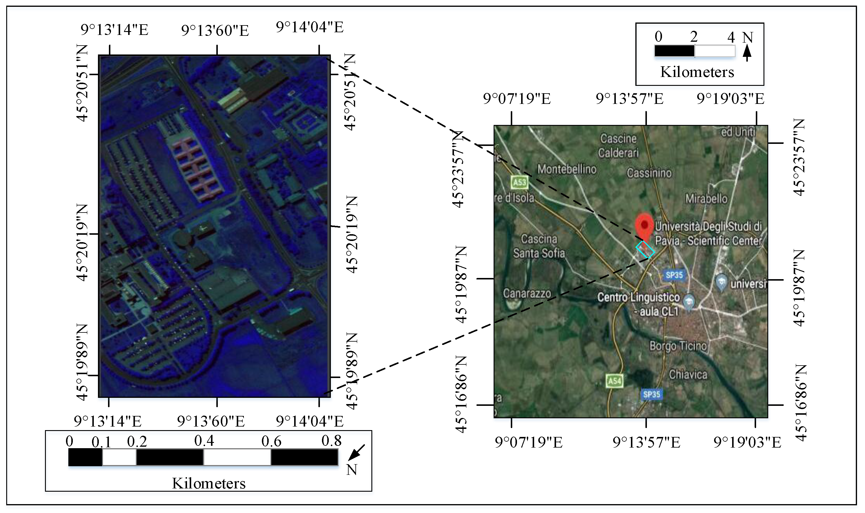
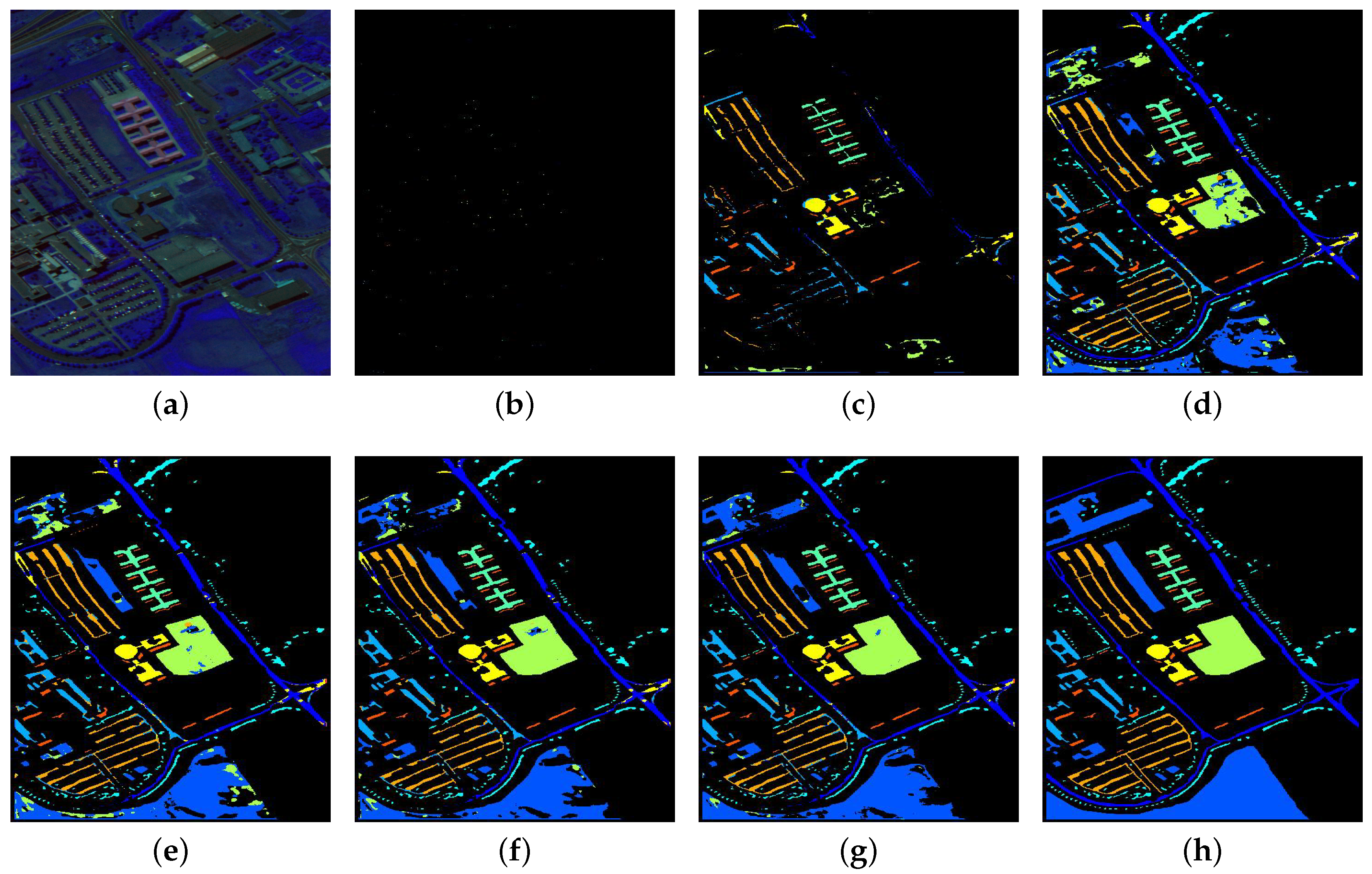
4.1.2. Pavia University Data Set

The Pavia University data set is shown in Figure 5. It consists of $610\times 610$ pixels and 103 spectral bands with a spatial resolution of $1.3$ m, but some samples in the image don’t contain any information and must be discarded before analysis. Its real category is divided into 9 with a total of 42,761 samples. The actual sample categories and numbers and colors are as Table 2.

Figure 5. Pavia University dataset: The left picture shows the pseudo-color of Pavia University dataset, and the right picture shows the geographical location of Pavia University dataset.

Table 2. Pavia University Data Set.

Serial Number	Colour	Class	Sample Number	Serial Number	Colour	Class	Sample Number
1		Asphalt	6548	6		Bare soil	5029
2		Meadows	18652	7		Bitumen	1330
3		Gravel	2099	8		Self-blocking bricks	3682
4		Trees	3064	9		Shadows	947
5		Painted metal sheets	1365

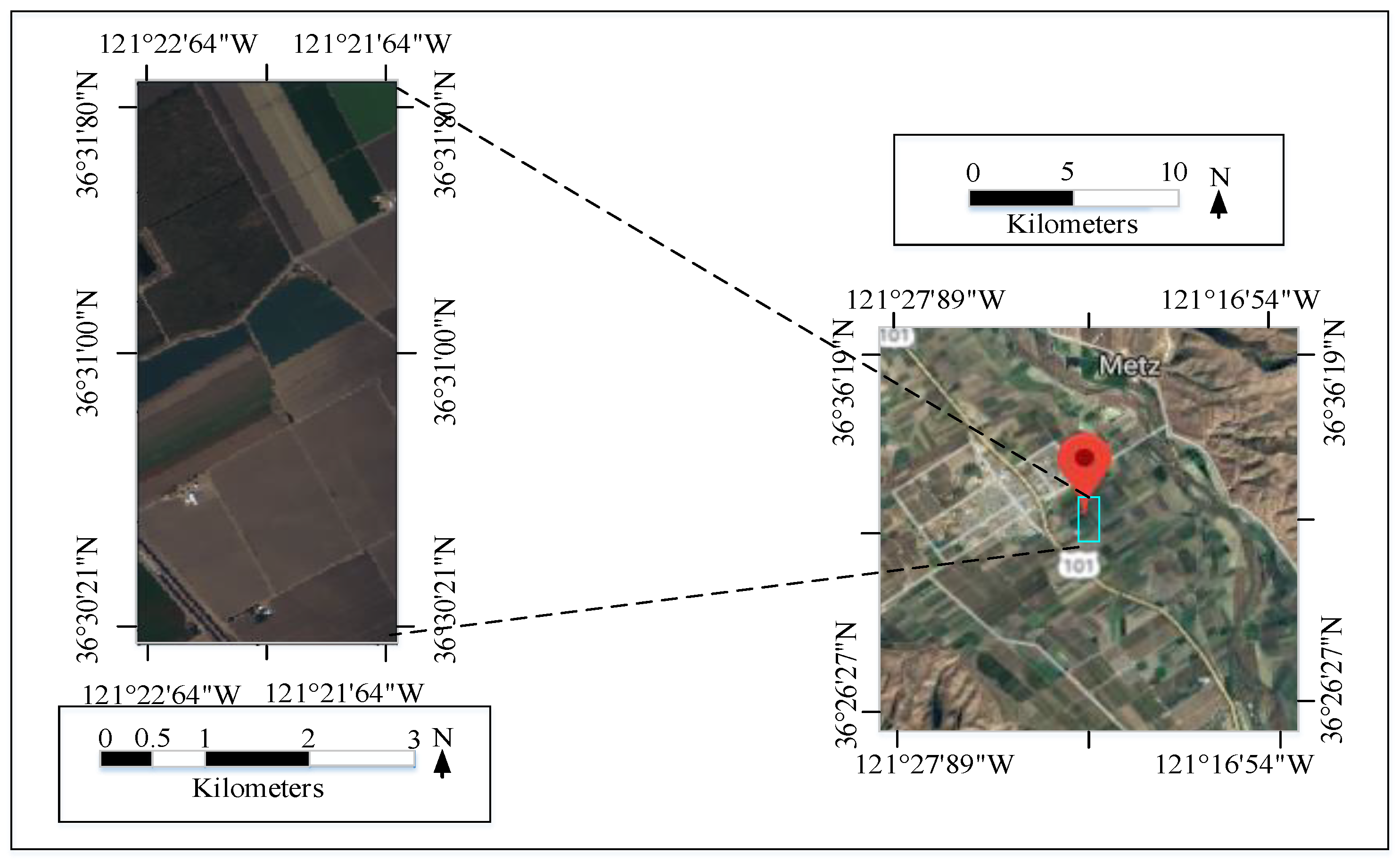
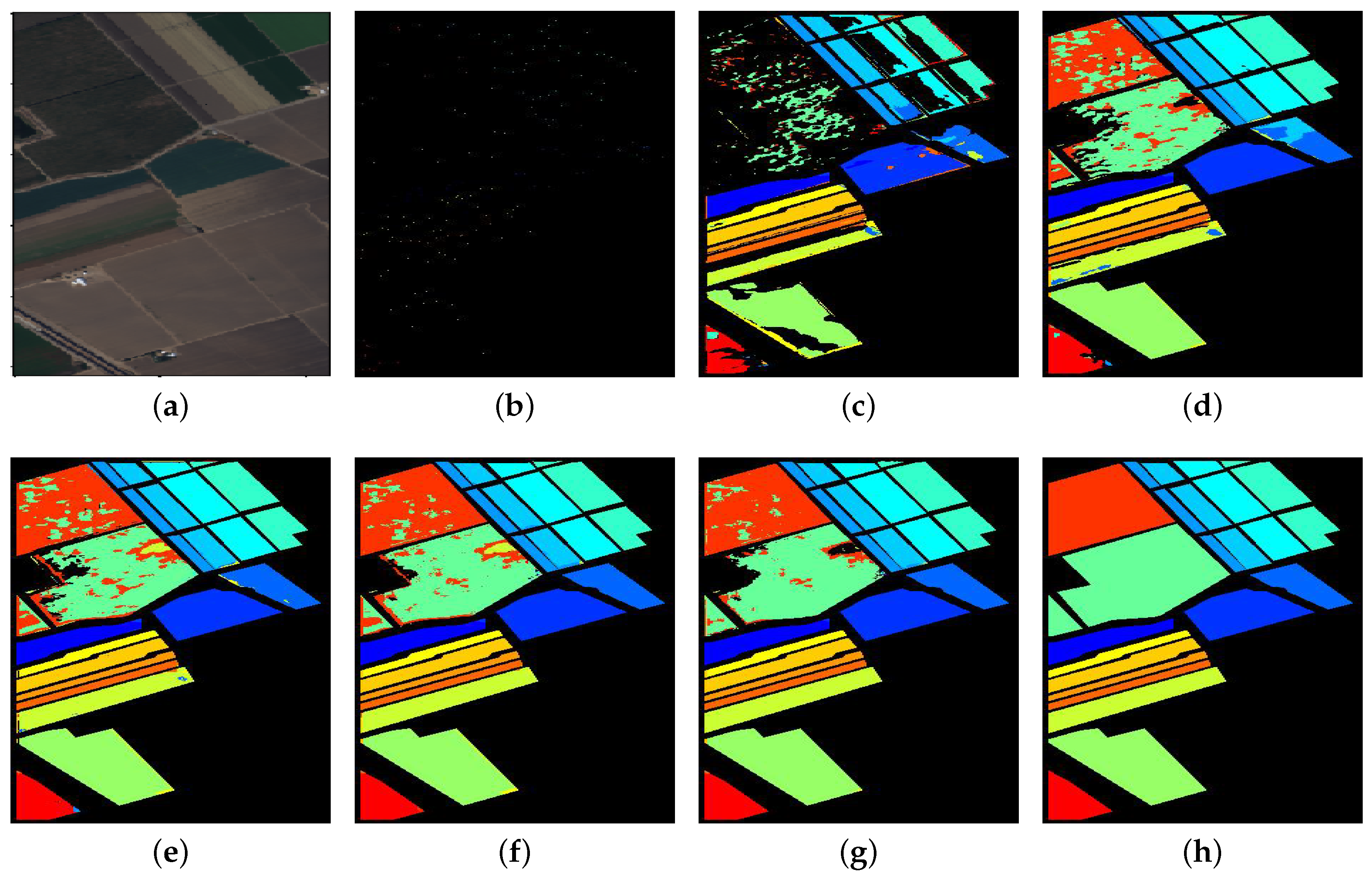
4.1.3. Salinas Scene Data Set

The Salinas Scene data set is shown in Figure 6. This scene was collected by the 224-band $AVIRIS$ sensor over Salinas Valley, California, and is characterized by high spatial resolution (3.7-meter pixels). The area covered comprises 512 lines by 217 samples.As with Indian Pines scene, we discarded the 20 water absorption bands. This image was available only as at-sensor radiance data. It includes vegetables, bare soils, and vineyard fields. Salinas groundtruth contains 16 classes.The actual sample categories and numbers and colors are as Table 3.

Figure 6. Salinas Scene dataset: The left picture shows the pseudo-color of Salinas Scene dataset, and the right picture shows the geographical location of Salinas Scene dataset.

Table 3. Salinas Scene Data Set.

Serial Number	Colour	Class	Sample Number	Serial Number	Colour	Class	Sample Number
1		Brocoli_green_weeds_1	2009	9		Soil_vinyard_develop	6203
2		Brocoli_green_weeds_2	3726	10		Corn_senesced_green_weeds	3278
3		Fallow	1976	11		Lettuce_romaine_4wk	1068
4		Fallow_rough_plow	1394	12		Lettuce_romaine_5wk	1927
5		Fallow_smooth	2678	13		Lettuce_romaine_6wk	916
6		Stubble	3959	14		Lettuce_romaine_7wk	1070
7		Celery	3579	15		Vinyard_untrained	7268
8		Grapes_untrained	11271	16		Vinyard_vertical_trellis	1807

4.2. Experimental Design

We compare the proposed method with several semi-supervised HSIc methods based on self-training frameworks, where these methods all use deep learning to extract spectral-spatial features. First, we compare our results with CDL, which is used as a benchmark for comparison. Then, we further compare the results with the classical semi-supervised classification method of SNI-L. SNI-L first uses the criteria based on spatial neighborhood information to infer the candidate set, and then assumes that the pixels which are spatially adjacent to the training sample can be labeled with the same label, and then automatically selects new samples from the candidate set. Finally, in order to maintain timeliness, we also compared with the newer method (SNI-unL) semi-supervised classification method. SNI-unL combines spatial neighborhood information of unlabeled samples with a classifier to enhance the classification ability of the selected unlabeled samples.

Different HSIc methods are compared based on three common metrics: $OA$ (overall accuracy), which measures the ratio of correctly classified samples in the entire test set; $AA$ (average accuracy), which is the classification average accuracy of each type; $Kappa$ indicator [55], which is calculated from the entries in the confusion matrix, and is a consistent robust measure of random classification.

In the process of extracting spectral-spatial features through CNN, normalization processing is added to the first, fourth, and seventh network layers. The feature maps are uniformly mapped to the interval [0, 1]. Because some feature maps are very large in amplitude and which can mask other feature maps, normalization can maintain a balance between feature maps.

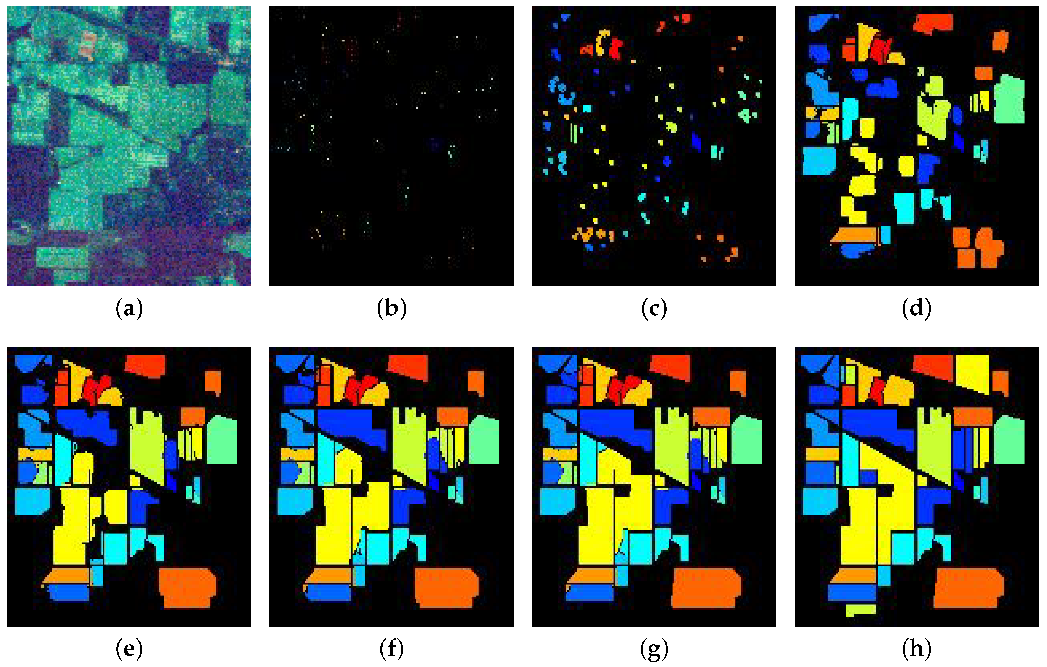
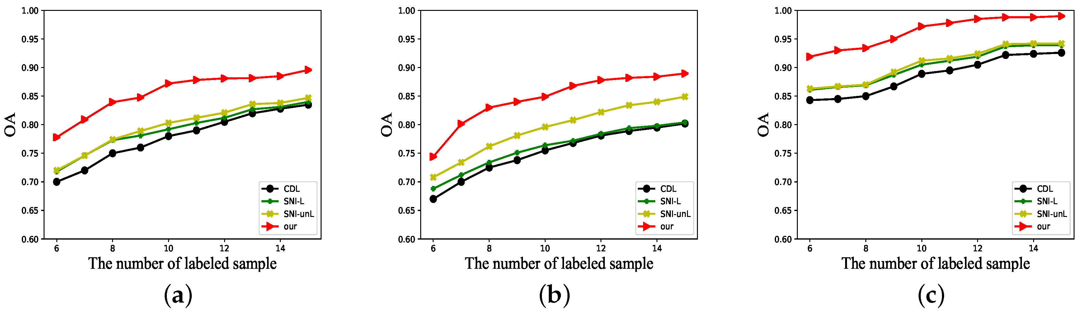
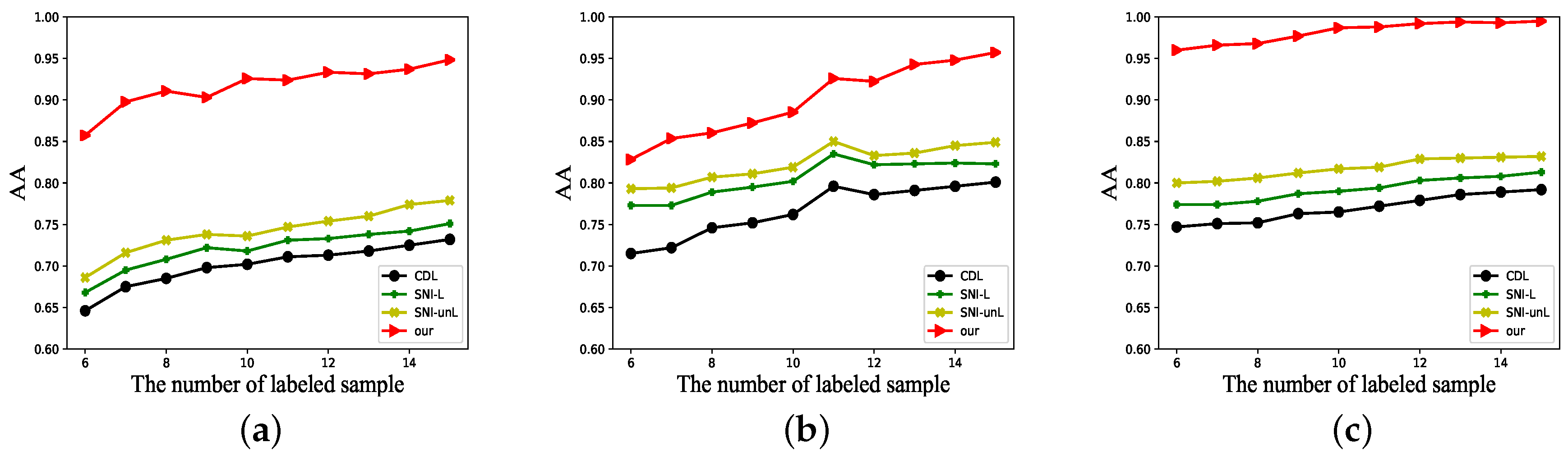
4.3. Experimental Result

First, we test the performance of our method and compare it with the CDL, SNI-L and SNI-unL algorithms. We randomly select 10 labeled samples for each class as the training set, and the rest of the data is used as the test set. The experimental results are shown in Figure 7, Figure 8 and Figure 9.

Figure 7. Indian Pines data set: (a) Sample band of Indian Pines dataset. (b) Small labeled dataset. (c) 1-output dataset. (d) 3-output dataset. (e) 5-output dataset. (f) 7-output dataset. (g) 9-output dataset. (h) Groundtruth of Indian Pines dataset.

Figure 8. Pavia University data set: (a) Sample band of Pavia University dataset. (b) Small labeled dataset. (c) 1-output dataset. (d) 3-output dataset. (e) 5-output data et. (f) 7-output dataset. (g) 9-output dataset. (h) Groundtruth of Pavia University dataset.

Figure 9. Salinas data set: (a) Sample band of Salinas dataset. (b) Small labeled dataset. (c) 1-output dataset. (d) 3-output dataset. (e) 5-output dataset. (f) 7-output dataset. (g) 9-output dataset. (h) Groundtruth of Salinas dataset.

Among them, Figure 7a is the Indian Pines data, Figure 7b is the selected small number of labeled sample sets, and Figure 7c–g are the algorithm iterations to the first, third, fifth, seventh, ninth rounds of output. And the classification accuracy ($OA$) of these iterations of the algorithm is shown in Table 4. Figure 7h is the ground truth of the Indian Pines data set. The algorithm stops when iterating to the 11th round, with a final classification accuracy ($OA$) of 87.35%.

Table 4. The classification accuracy of the iteration round and the variance of the experimental.

Data	First	Third	Fifth	Seventh	Ninth	Variance
Indian Pines	23.25%	72.73%	81.57%	85.45%	86.42%	0.03%
Pavia University	12.30%	55.23%	70.36%	78.88%	81.69%	0.17%
Salinas Scene	39.91%	82.81%	89.04%	92.66%	93.97%	0.005%

Among them, Figure 8a is the Pavia University data, Figure 8b is the selected small number of labeled sample sets, and Figure 8c–g are the algorithm iterations to the first, third, fifth, seventh, ninth rounds of output. And the classification accuracy ($OA$) of these iterations of the algorithm is shown in Table 4. Figure 8h is the ground truth of the Pavia data set. The algorithm stops when iterating to the 12th round, with a final classification accuracy ($OA$) of 85.63%.

Among them, Figure 9a is the Salinas data, Figure 9b is the selected small number of labeled sample sets, and Figure 9c–g are the algorithm iterations to the first, third, fifth, seventh, ninth rounds of output. And the classification accuracy ($OA$) of these iterations of the algorithm is shown in Table 4. Figure 9h is the ground truth of the Salinas data set. The algorithm stops when iterating to the 11th round, with a final classification accuracy ($OA$) of 97.37%.

The average $OA$, $AA$, and $Kappa$ obtained in the experiment five times are shown in Table 5.

Table 5. Average $OA$, $AA$, and $Kappa$ for the Indian Pines, Pavia University and Salinas Scene datas.

Data	Measurement	CDL	SNI-L	SNI-unL	Our Method
Indian Pines	OA	0.7751 ± 0.0270	0.7881 ± 0.0220	0.8062 ± 0.0270	0.8755 ± 0.0126
	AA	0.7751 ± 0.0270	0.7757 ± 0.0223	0.7753 ± 0.0350	0.9237 ±  0.0057
	Kappa	0.7496 ± 0.0300	0.7818 ± 0.0200	0.7818 ± 0.0300	0.8608 ±  0.0138
Pavia University	OA	0.7508 ± 0.0304	0.7556 ± 0.0471	0.7872 ± 0.0425	0.8178 ±  0.0372
	AA	0.7508 ± 0.0304	0.7841 ± 0.0258	0.8031 ± 0.0302	0.8835 ±  0.0283
	Kappa	0.6910 ± 0.0300	0.6981 ± 0.0500	0.7341 $\pm 0.0500$	0.7759 ±  0.0429
Salinas Scene	OA	0.8890 ± 0.0230	0.9050 ± 0.0210	0.9120 ± 0.0240	0.9733 ±  0.0061
	AA	0.7650 ± 0.0130	0.7900 ± 0.0121	0.8170 ± 0.0170	0.9878 ±  0.0023
	Kappa	0.8390 ± 0.0110	0.8410 ± 0.0100	0.8430 ± 0.0170	0.9704 ±  0.0067

For the Indian Pines data set, we use $31\times 31$ window for spatially constrained, and the CDL parameters are set according to their original paper, and the first layer window size is set to $9\times 9$. For the Pavia University data set, the spatially constrained window size is set to $47\times 47$ and the first layer window size is set to $21\times 21$.

We can get from the above experimental results: Our method suppresses the generation of pseudo labels by adding semantic attribute constraints and spatial constraints. In each iteration, better representation features are extracted from the CNN, which helps the classifier to better classify. As can be seen from the results of $OA$, $AA$ and $Kappa$, when the initial labels (10 per class) are very small, our method performs well. We obtained the variance for the results of the five experiments. It can be seen from the variance of Table 4 that our method is relatively stable.

5. Discussion

For this method, the number of initial labels selected has a large impact on performance. In order to investigate the effect of the number of initial labels on the labeling results, we conduct experimental validation. Each time the number of initial labels for each class is selected from 6 to 15, the values of the three indicators $OA$, $AA$ and $Kappa$ are obtained. We conduct five experiments to obtain the mean of the three indicators, then the number of initial labels with the x-axis as the initial selection, and the y-axis for the corresponding $OA$, $AA$, $Kappa$ indicators to draw their images. From the image index curve, it can be obtained that the number of initial labels does have an effect on the labeling result. Figure 10, Figure 11 and Figure 12 correspond to changes in $OA$, $AA$, and $Kappa$ indicators for the classification results of the four classification methods.

Figure 10. (a) Indian Pines. (b) Pavia University. (c) Salinas Scene.

Figure 11. (a) Indian Pines. (b) Pavia University. (c) Salinas Scene.

Figure 12. (a) Indian Pines. (b) Pavia University.(c) Salinas Scene.

The Figure 10 shows the changes in the $OA$ indicators of the classification results of four classification methods, such as CDL, SNI-L and SNI-unL, when initially selecting different number of labels. It can be seen that, overall, the $OA$ increases with the number of initial labels increases, indicating that the more the number of initial labels, the higher the ratio of correctly classified samples in the entire test set. Moreover, the $OA$ indicator of our method is always higher than other methods, which indicates that our classification method is superior.

The Figure 11 shows the change in the $AA$ indicator for the number of different initial labels. The higher the rate, the better the classification effect for each class. It can be seen that like $OA$, it also increases with the number of initial labels increases, reflecting that the algorithm’s classification effect for each class is increasing. The $AA$ index of our method is much higher than other methods, and it can be seen that our method is more friendly to all classes.

Similarly, the Figure 12 shows how the $Kappa$ indicator changes with the number of labels initially selected varies. We know that $Kappa$ can be divided into five groups to indicate different levels of consistency: 0.0–0.20 is extremely low, 0.21–0.40 is normal, 0.41–0.60 is medium, 0.61–0.80 is highly consistent, and 0.81–1 is almost identical. It can be seen that almost all algorithm results increase with the number of initial labels increasing. Our method $Kappa$ indicator is almost between 0.81 and 1, which is always higher than other algorithms, that is, our method has higher classification consistency.

6. Conclusions

In this paper, we introduce a novel semi-supervised classification algorithm for HSIc based on the cooperation between deep learning models and clustering. The algorithm is based on a self-training algorithm for solving the problem that hyperspectral images contain a large number of unlabeled samples, and the cost of labeled samples is too high. First, we use CNN to extract spatial-spectral features. Afterward, the extracted spectral-spatial features are used for semantic constraint clustering. The novelty of this paper is that the hyperspectral image is divided into several spectral slices, and each spectral slice is separately subjected to semantic constraint clustering, and the clustering results are compared. Just the samples in the clustering results that are assigned to the same semantic class are used as the clustering results for the entire hyperspectral image. In hyperspectral images, adjacent pixels have the same class, so we introduce local decisions to smooth the pseudo labels after obtaining the clustering results for the entire image. Our algorithm is compared to CDL, SNI-L and SNI-unL respectively. The average of the three indicators of our algorithm $OA$, $AA$ and $Kappa$ is higher than the other three algorithms, and by calculating the variance of our method, we can see that our algorithm is superior.

The framework has some drawbacks: (1) This paper is based on a self-training algorithm. The shortcoming of this algorithm is that the mislabeled samples in the previous iteration will affect the later iterative process and will increase its impact. At present, there is no way to completely solve this problem. If the following academia solves this problem, we will continue to optimize the algorithm in this article. Our method can only reduce the error rate by a part. Later we might consider adding new constraints to improve classification accuracy, or consider adopting a new advanced framework. (2) The problem of boundaries between different scenes, adjacent samples have different classes. Adjacent samples have a large overlap of image patches, so the features extracted by CNN may be similar. It can be seen from the experimental results of the three data sets that the Indian Pines and Salinas Scene scenes are relatively simple and the classification accuracy ($OA$) is relatively high. The Pavia University scene is complex and the classification accuracy ($OA$) is relatively low.

References

- Jiang, J.; Chen, C.; Yu, Y.; Jiang, X.; Ma, J. Spatial-aware Collaborative Representation for Hyperspectral Remote Sensing Image Classification. IEEE Geosci. Remote Sens. Lett. 2017, 14, 404–408. [Google Scholar] [CrossRef]
- Jiang, J.; Ma, J.; Wang, Z.; Chen, C.; Liu, X. Hyperspectral Image Classification in the Presence of Noisy Labels. IEEE Trans. Geosci. Remote Sens. 2018, 57, 851–865. [Google Scholar] [CrossRef]
- Liu, J.; Zhang, X.; Zhang, J.; An, J.; Li, C.; Gao, L. Hyperspectral Image Classification Based on Long Short Term Memory Network. In Proceedings of the Fifth International Workshop on Earth Observation and Remote Sensing Applications (EORSA), Xi’an, China, 18–20 June 2018; pp. 1–5. [Google Scholar]
- Matsuki, T.; Yokoya, N.; Iwasaki, A. Hyperspectral Tree Species Classification of Japanese Complex Mixed Forest With the Aid of LiDAR Data. IEEE J. Sel. Top. Appl. Earth Obs. Remote Sens. 2015, 8, 2177–2187. [Google Scholar] [CrossRef]
- Shafri, H.Z.; Taherzadeh, E.; Mansor, S.; Ashurov, R. Hyperspectral Remote Sensing of Urban Areas: An Overview of Techniques and Applications. Res. J. Appl. Sci. Eng. Technol. 2012, 4, 1557–1565. [Google Scholar]
- Wu, Y.; Ma, W.; Gong, M.; Su, L.; Jiao, L. A Novel Point-Matching Algorithm Based on Fast Sample Consensus for Image Registration. IEEE Geosci. Remote. Sens. Lett. 2014, 12, 43–47. [Google Scholar] [CrossRef]
- Wu, Y.; Ma, W.; Gong, M.; Li, H.; Jiao, L. Novel Fuzzy Active Contour Model with Kernel Metric for Image Segmentation. Appl. Soft Comput. 2015, 34, 301–311. [Google Scholar] [CrossRef]
- Wu, Y.; Ma, W.; Miao, Q.; Wang, S. Multimodal Continuous ant Colony Optimization for Multisensor Remote Sensing Image Registration with Local Search. Swarm Evol. Comput. 2017, 47, 89–95. [Google Scholar] [CrossRef]
- An, J.; Lei, J.; Song, Y.; Zhang, X.; Guo, J. Tensor Based Multiscale Low Rank Decomposition for Hyperspectral Images Dimensionality Reduction. Remote Sens. 2019, 11, 1485. [Google Scholar] [CrossRef]
- Zhang, X.; Han, Y.; Huyan, N.; Li, C.; Feng, J.; Gao, L.; Ma, X. Spatial-Spectral Graph-Based Nonlinear Embedding Dimensionality Reduction for Hyperspectral Image Classificaiton. In Proceedings of the IEEE International Geoscience and Remote Sensing Symposium (IGARSS), Valencia, Spain, 22–27 July 2018; pp. 8472–8475. [Google Scholar]
- Chen, Y.; Zhao, X.; Jia, X. Spectral–spatial Classification of Hyperspectral Data Based on Deep Belief Network. IEEE J. Sel. Top. Appl. Earth Obs. Remote Sens. 2015, 8, 2381–2392. [Google Scholar] [CrossRef]
- Kang, X.; Xiang, X.; Li, S.; Benediktsson, J.A. PCA-based Edge-preserving Features for Hyperspectral Image Classification. IEEE Trans. Geosci. Remote Sens. 2017, 55, 7140–7151. [Google Scholar] [CrossRef]
- Jiang, J.; Ma, J.; Chen, C.; Wang, Z.; Cai, Z.; Wang, L. SuperPCA: A Superpixelwise PCA Approach for Unsupervised Feature Extraction of Hyperspectral Imagery. IEEE Trans. Geosci. Remote Sens. 2018, 56, 1–13. [Google Scholar] [CrossRef]
- Villa, A.; Benediktsson, J.A.; Chanussot, J.; Jutten, C. Hyperspectral Image Classification With Independent Component Discriminant Analysis. IEEE Trans. Geosci. Remote Sens. 2011, 49, 4865–4876. [Google Scholar] [CrossRef]
- Zhou, P.; Han, J.; Cheng, G.; Zhang, B. Learning Compact and Discriminative Stacked Autoencoder for Hyperspectral Image Classification. IEEE Trans. Geosci. Remote Sens. 2019, 57, 4823–4833. [Google Scholar] [CrossRef]
- Abdel-Zaher, A.M.; Eldeib, A.M. Breast Cancer Classification using Deep Belief Networks. Expert Syst. Appl. 2016, 46, 139–144. [Google Scholar] [CrossRef]
- Simonyan, K.; Zisserman, A. Very Deep Convolutional Networks for Large-scale Image Recognition. arXiv 2014, arXiv:1409.1556. [Google Scholar]
- Zhang, X.; Li, X.; An, J.; Gao, L.; Hou, B.; Li, C. Natural Language Description of Remote Sensing Images Based on Deep Learning. In Proceedings of the IEEE International Geoscience and Remote Sensing Symposium (IGARSS), Fort Worth, TX, USA, 23–28 July 2017; pp. 4798–4801. [Google Scholar]
- Pleva, M.; Liao, Y.F.; Hsu, W.; Hladek, D.; Stas, J.; Viszlay, P.; Lojka, M.; Juhar, J. Towards Slovak-English-Mandarin Speech Recognition Using Deep Learning. In Proceedings of the International Symposium ELMAR, Zadar, Croatia, 16–19 September 2018; pp. 151–154. [Google Scholar]
- Ma, X.; Wang, H.; Wang, J. Semisupervised Classification for Hyperspectral Image Based on Multi-Decision Labeling and Deep Feature Learning. J. Photogram. Remote Sens. 2016, 120, 99–107. [Google Scholar] [CrossRef]
- Duan, P.; Kang, X.; Li, S.; Benediktsson, J.A. Multi-Scale Structure Extraction for Hyperspectral Image Classification. In Proceedings of the IEEE International Geoscience and Remote Sensing Symposium (IGARSS), Valencia, Spain, 22–27 July 2018; pp. 5724–5727. [Google Scholar]
- Senthilnath, J.; Kulkarni, S.; Benediktsson, J.A.; Yang, X.S. A Novel Approach for Multispectral Satellite Image Classification Based on the Bat Algorithm. IEEE Geosci. Remote Sens. Lett. 2016, 13, 599–603. [Google Scholar] [CrossRef]
- Essa, A.; Sidike, P.; Asari, V. Volumetric Directional Pattern for Spatial Feature Extraction in Hyperspectral Imagery. IEEE Geosci. Remote Sens. Lett. 2017, 14, 1056–1060. [Google Scholar] [CrossRef]
- Sidike, P.; Chen, C.; Asari, V.; Xu, Y.; Li, W. Classification of hyperspectral image using multiscale spatial texture features. In Proceedings of the Workshop on Hyperspectral Image and Signal Processing: Evolution in Remote Sensing (WHISPERS), Los Angeles, CA, USA, 21–24 August 2016; pp. 1–4. [Google Scholar]
- Lee, H.; Kwon, H. Going Deeper with Contextual CNN for Hyperspectral Image Classification. IEEE Trans. Image Process. 2017, 26, 4843–4855. [Google Scholar] [CrossRef]
- Zhang, H.; Li, Y.; Zhang, Y.; Shen, Q. Spectral-Spatial Classification of Hyperspectral Imagery Using a Dual-Channel Convolutional Neural Network. Remote Sens. Lett. 2017, 8, 438–447. [Google Scholar] [CrossRef]
- Ma, W.; Yang, Q.; Wu, Y.; Zhao, W.; Zhang, X. Double-Branch Multi-Attention Mechanism Network for Hyperspectral Image Classification. Remote Sens. 2019, 11, 1307. [Google Scholar] [CrossRef]
- Cao, J.; Chen, Z.; Wang, B. Deep Convolutional Networks with Superpixel Segmentation for Hyperspectral Image Classification. In Proceedings of the IEEE International Geoscience and Remote Sensing Symposium (IGARSS), Beijing, China, 10–15 July 2016; pp. 3310–3313. [Google Scholar]
- Yang, J.; Zhao, Y.Q.; Chan, J.C.W. Learning and Transferring Deep Joint Spectral–Spatial Features for Hyperspectral Classification. IEEE Trans. Geosci. Remote Sens. 2017, 55, 4729–4742. [Google Scholar] [CrossRef]
- Meer, F.D.V.D.; Werff, H.M.A.V.D.; Ruitenbeek, F.J.A.V.; Hecker, C.A.; Bakker, W.H.; Noomen, M.F.; Meijde, M.V.D.; Carranza, E.J.M.; Smeth, J.B.D.; Woldai, T. Multi- and Hyperspectral Geologic Remote Sensing: A Review. Int. J. Appl. Earth Obs. Geoinf. 2012, 14, 112–128. [Google Scholar] [CrossRef]
- Zhang, C.; Kovacs, J.M. The application of small unmanned aerial systems for precision agriculture: A review. Precis. Agric. 2012, 13, 693–712. [Google Scholar] [CrossRef]
- Pan, B.; Shi, Z.; An, Z.; Jiang, Z.; Ma, Y. A Novel Spectral-Unmixing-Based Green Algae Area Estimation Method for GOCI Data. IEEE J. Sel. Top. Appl. Earth Obs. Remote Sens. 2016, 10, 437–449. [Google Scholar] [CrossRef]
- Melgani, F.; Bruzzone, L. Classification of Hyperspectral Remote Sensing Images with Support Vector Machines. IEEE Trans. Geosci. Remote Sens. 2004, 42, 1778–1790. [Google Scholar] [CrossRef]
- Tarabalka, Y.; Fauvel, M.; Chanussot, J.; Benediktsson, J.A. SVM-and MRF-based Method for Accurate Classification of Hyperspectral Images. IEEE Geosci. Remote Sens. Lett. 2010, 7, 736–740. [Google Scholar] [CrossRef]
- Camps-Valls, G.; Tuia, D.; Bruzzone, L.; Benediktsson, J.A. Advances in Hyperspectral Image Classification: Earth Monitoring with Statistical Learning Methods. IEEE Signal Process. Mag. 2013, 31, 45–54. [Google Scholar] [CrossRef]
- Acquarelli, J.; Marchiori, E.; Buydens, L.M.; Tran, T.; van Laarhoven, T. Convolutional Neural Networks and Data Augmentation for Spectral-Spatial Classification of Hyperspectral Images. Networks 2017, 16, 21. [Google Scholar]
- Chen, C.; Ma, Y.; Ren, G. A Convolutional Neural Network with Fletcher–Reeves Algorithm for Hyperspectral Image Classification. Remote Sens. 2019, 11, 1325. [Google Scholar] [CrossRef]
- Makantasis, K.; Karantzalos, K.; Doulamis, A.; Doulamis, N. Deep Supervised Learning for Hyperspectral Data Classification through Convolutional Neural Networks. In Proceedings of the IEEE International Geoscience and Remote Sensing Symposium (IGARSS), Milan, Italy, 26–31 July 2015; pp. 4959–4962. [Google Scholar]
- Wang, Z.; Du, B.; Zhang, L.; Zhang, L.; Jia, X. A Novel Semisupervised Active-Learning Algorithm for Hyperspectral Image Classification. IEEE Trans. Geosci. Remote Sens. 2017, 55, 3071–3083. [Google Scholar] [CrossRef]
- Tran, T.N.; Wehrens, R.; Hoekman, D.H.; Buydens, L.M. Initialization of Markov Random Field Clustering of Large Remote Sensing Images. IEEE Trans. Geosci. Remote Sens. 2005, 43, 1912–1919. [Google Scholar] [CrossRef]
- Cao, X.; Xu, Z.; Meng, D. Spectral-Spatial Hyperspectral Image Classification via Robust Low-Rank Feature Extraction and Markov Random Field. Remote Sens. 2019, 11, 1565. [Google Scholar] [CrossRef]
- Lu, T.; Li, S.; Fang, L.; Jia, X.; Benediktsson, J.A. From Subpixel to Superpixel: A NovelFfusion Framework for Hyperspectral Image Classification. IEEE Trans. Geosci. Remote Sens. 2017, 55, 4398–4411. [Google Scholar] [CrossRef]
- Ma, X.; Geng, J.; Wang, H. Hyperspectral Image Classification via Contextual Deep Learning. EURASIP J. Image Video Process. 2015, 2015, 1–12. [Google Scholar] [CrossRef]
- Dópido, I.; Li, J.; Marpu, P.R.; Plaza, A.; Dias, J.M.B.; Benediktsson, J.A. Semisupervised Self-Learning for Hyperspectral Image Classification. IEEE Trans. Geosci. Remote Sens. 2013, 51, 4032–4044. [Google Scholar] [CrossRef]
- Tan, K.; Hu, J.; Li, J.; Du, P. A Novel Semi-supervised Hyperspectral Image Classification Approach Based on Spatial Neighborhood Information and Classifier Combination. ISPRS J. Photogramm. Remote Sens. 2015, 105, 19–29. [Google Scholar] [CrossRef]
- Dempster, A.P.; Laird, N.M.; Rubin, D.B. Maximum Likelihood from Incomplete Data via the EM Algorithm. J. R. Stat. Soc. 1977, 39, 1–38. [Google Scholar]
- Bruzzone, L.; Chi, M.; Marconcini, M. Transductive SVMs for Semisupervised Classification of Hyperspectral Data. In Proceedings of the IEEE International Geoscience and Remote Sensing Symposium (IGARSS), Seoul, Korea, 29 July 2005; Volume 1, pp. 164–167. [Google Scholar]
- Camps-Valls, G.; Marsheva, T.V.B.; Zhou, D. Semi-Supervised Graph-Based Hyperspectral Image Classification. IEEE Trans. Geosci. Remote Sens. 2007, 45, 3044–3054. [Google Scholar] [CrossRef]
- Li, F.; Clausi, D.A.; Xu, L.; Wong, A. ST-IRGS: A Region-based Self-training Algorithm Applied to Hyperspectral Image Classification and Segmentation. IEEE Trans. Geosci. Remote Sens. 2017, 56, 3–16. [Google Scholar] [CrossRef]
- LeCun, Y.; Bottou, L.; Bengio, Y.; Haffner, P. Gradient-based Learning Applied to Document Recognition. Proc. IEEE 1998, 86, 2278–2324. [Google Scholar] [CrossRef]
- Bengio, Y.; Courville, A.; Vincent, P. Representation Learning: A Review and New Perspectives. IEEE Trans. Pattern Anal. Mach. Intell. 2013, 35, 1798–1828. [Google Scholar] [CrossRef] [PubMed]
- Long, J.; Shelhamer, E.; Darrell, T. Fully convolutional networks for semantic segmentation. In Proceedings of the IEEE Conference on Computer Vision and Pattern Recognition, Boston, MA, USA, 7–12 June 2015; pp. 3431–3440. [Google Scholar]
- Qin, C.; Gong, M.; Wu, Y.; Tian, D.; Zhang, P. Efficient Scene Labeling via Sparse Annotations. In Proceedings of the Workshops at the Thirty-Second AAAI Conference on Artificial Intelligenc, Hilton New Orleans Riverside, New Orleans, LA, USA, 2–3 February 2018; pp. 194–201. [Google Scholar]
- Rumelhart, D.E.; Hinton, G.E.; Williams, R.J. Learning Representations by Back-propagating Errors. Cogn. Model. 1986, 323, 533–536. [Google Scholar] [CrossRef]
- Viera, A.J.; Garrett, J.M. Understanding Interobserver Agreement: The Kappa Statistic. Family Med. 2005, 37, 360–363. [Google Scholar]
© 2020 by the authors. Licensee MDPI, Basel, Switzerland. This article is an open access article distributed under the terms and conditions of the Creative Commons Attribution (CC BY) license (http://creativecommons.org/licenses/by/4.0/).