Article

Understanding Current and Future Fragmentation Dynamics of Urban Forest Cover in the Nanjing Laoshan Region of Jiangsu, China

1
College of Forestry, Nanjing Forestry University, Nanjing 210037, China
2
Co-Innovation Center for Sustainable Forestry in Southern China, Nanjing Forestry University, Nanjing 210037, China
3
Department of Geographical Sciences, University of Maryland, College Park, MD 20742, USA
4
Key Laboratory of Land Surface Pattern and Simulation, Institute of Geographic Sciences and Natural Resources Research, Chinese Academy of Sciences, Beijing 100101, China
*
Author to whom correspondence should be addressed.
Remote Sens. 2020, 12(1), 155; https://doi.org/10.3390/rs12010155
Submission received: 23 October 2019 / Revised: 12 December 2019 / Accepted: 31 December 2019 / Published: 2 January 2020
(This article belongs to the Special Issue Monitoring Forest Change with Remote Sensing)

Abstract

:
Accurate acquisition of the spatiotemporal distribution of urban forests and fragmentation (e.g., interior and intact regions) is of great significance to contributing to the mitigation of climate change and the conservation of habitat biodiversity. However, the spatiotemporal pattern of urban forest cover changes related with the dynamics of interior and intact forests from the present to the future have rarely been characterized. We investigated fragmentation of urban forest cover using satellite observations and simulation models in the Nanjing Laoshan Region of Jiangbei New Area, Jiangsu, China, during 2002–2023. Object-oriented classification-based land cover maps were created to simulate land cover changes using the cellular automation-Markov chain (CA-Markov) model and the state transition simulation modeling. We then quantified the forest cover change by the morphological change detection algorithm and estimated the forest area density-based fragmentation patterns. Their relationships were built through the spatial analysis and statistical methods. Results showed that the overall accuracies of actual land cover maps were approximately 83.75–92.25% (2012–2017). The usefulness of a CA-Markov model for simulating land cover maps was demonstrated. The greatest proportion of forest with a low level of fragmentation was captured along with the decreasing percentage of fragmented area from 81.1% to 64.1% based on high spatial resolution data with the window size of 27 pixels × 27 pixels. The greatest increase in fragmentation (3% from 2016 to 2023) among the changes between intact and fragmented forest was reported. However, intact forest was modeled to have recovered in 2023 and restored to 2002 fragmentation levels. Moreover, we found 58.07 km2 and 0.35 km2 of interior and intact forests have been removed from forest area losses and added from forest area gains. The loss rate of forest interior and intact area exceeded the rate of total forest area loss. However, their approximate ratio (1) implying the loss of forest interior and intact area would have slight fragmentation effects on the remaining forests. This analysis illustrates the achievement of protecting and restoring forest interior; more importantly, excessive human activities in the surrounding area had been avoided. This study provides strategies for future forest conservation and management in large urban regions.

Graphical Abstract

1. Introduction

Natural and anthropogenic disturbances during the process of urbanization strongly affect biodiversity and ecosystem dynamics in urban ecosystems, through the alteration of species richness, carbon stocks, and microclimates [1,2]. Forested urban ecosystems are vulnerable to forest cover loss and fragmentation [3,4,5]. Although commonly adopted, forest cover change by itself is an incomplete indicator of forest capability in sustaining ecological services, since forest cover decrease does not always result in increase of ecological risk [6].
Existing research has identified forest interior (i.e., interior and intact forests) as an indicator of habitat quality and forest fragmentation [7]. Interior and intact regions, as two types of fragmentation (little or no fragmented forests), can be defined as the forest areas that exist in forest-dominated neighborhoods of a specified size, and are not affected by nearby non-forested or disturbed forest habitats [8]. A variety of physical and biological mechanisms in fragmented forests can limit the ecological functions of those forests, although varied by conditions in forest interior environments [9,10,11]. Therefore, accurate assessment of forest interior is beneficial for monitoring forest change and fragmentation magnitude, as well as maintaining ecological values of the forests [6,7,12]. Moreover, assessing current and future forest fragmentation patterns related to forest cover change in densely populated and rapidly developing regions, is critical for understanding the impacts of economic development on urban ecosystems and designing policies to reduce the ecological risks [12,13,14,15,16].
Aerial and satellite-based remote sensing has been commonly used for monitoring urban forest cover change and understanding urban forest cover and fragmentation patterns [17,18]. Individual year or perennial data that employ moderate to coarse resolution imagery have been frequently investigated to track forest change and monitor fragmentation [19,20,21,22]. Multi-temporal high resolution satellite imagery and light detection and ranging (LiDAR) data also play an important role in capturing accurate and detailed spatial patterns of fragmentation of urban forest cover, although the application of these datasets are limited in their spatial and temporal coverage [23,24,25,26].
Future changes in forest cover can be predicted using the knowledge gained from historical post-classification datasets and remote sensing observations [27,28,29]. The spatial and state transition-based change process modeling such as cellular automata (CA) and agent-based models, or their mixtures, are the most widely used methods in land cover change modeling [28,30]. For example, a state-and-transition simulation model (STSM) was designed to overcome the limitations of Markov chains [31] for landscape change modeling by combining features with a CA model [32]. However, the cellular automation-Markov chain (CA-Markov) [28,33] and STSM [34,35] models differ in the representation of spatial interaction [34], and their performances in predicting land cover change are largely unknown for urban forest ecosystems. Traditionally, a simple overlay of classified maps has been used in some studies to monitor post-classification change dynamics [36]. Mis-registration in maps and mixed pixels, however, will inevitably lead to spurious changes [36,37]. Filters and simple morphological operations can omit change information, which can affect forest cover patterns [36]. Therefore, morphological change detection methods have been designed to overcome the above deficiencies [38,39]. Thus, coalescing supervised object-based image classification as well as simulation methods for morphological post-processing of change detection used to generate subtle land cover changes in the urban forest are emerging. This is done because of the high level of accuracy and spatiotemporal suitability, as well as the continuity of data, are required to develop modeling of urban forest fragmentation patterns [25].
Fragmentation metrics and analysis models have been widely utilized in existing studies to monitor landscape fragmentation patterns from local to global scales [19,20,40,41,42,43]. Zhou et al. [22] explored the statistical relationships between urban expansion and forest loss and landscape metrics-based fragmentation using correlation analysis. It has been found that urban expansion was a major driver of forest loss, and its cover has impacts on forest fragmentation; however, the relationships between the spatiotemporal pattern of forest loss and fragmentation were rarely examined [22]. The moving window-based forest area density (FAD) method has the ability to quantify spatiotemporal changes of fragmentation by identifying its time and location. However, an attempt to redefine the percentage threshold for fragmentation classes to determine the magnitude of fragmentation (i.e., interiors and fragmented forests) and to integrate with multi-source-based forest loss and gain may provide new insights and advance monitoring of local-scale patterns [21,44].
China has several types of protected forests and other types of landscapes, such as the National New Areas and National Forest Parks of China [45,46]. Established in 2015, the Nanjing Jiangbei New Area (NJNA), Jiangsu Province, China is being developed to become China’s important scientific and technological innovation base and an advanced industrial base with an ecologically sound and livable civic environment (www.najing.gov.cn). How to maintain a balance between the forest interior and the forest itself in the Nanjing Laoshan Region (NLR) of Jiangbei New Area, eastern China, is a critical issue that needs to be addressed to allow forest managers and policy-makers to create effective strategies designed to manage urban forests sustainably [13,15,25,47]. This study aims to map forest cover change and fragmentation patterns with high-resolution remotely sensed data for the Nanjing Laoshan Region at a regional level during 2002–2023. Specifically, we focus on: (1) mapping recent land cover based on high resolution imagery and simulating future land cover change by using two landscape predictive models; (2) comparing FAD-based fragmentation patterns derived from medium or high resolution data; and (3) quantifying the spatial pattern of forest loss and gain based on the dynamics of forest interior and intact areas.

2. Materials and Methods

2.1. Study Area

Our study area covered the Nanjing Laoshan Region (NLR; 32°00′N–32°11′N, 118°20′E–118°42′E, 300 km2) located in the Jiangbei New Area in Nanjing near the Yangtze River in Jiangsu, China (Figure 1). The main part of Laoshan Region is Mount Laoshan Forest Park (MLFP). Located in the east of the region, it is the largest forest park in Nanjing with 90.3% forest cover (www.pukou.gov.cn). Deciduous and evergreen broad-leaved mixed forests are widespread within the NLR. The elevation ranges from 7 to 442 m above sea level. With a subtropical monsoon climate, this region has an annual mean temperature of about 15.3 °C and annual mean precipitation of about 1000 mm. The rainy season from April to July provides approximately 70% of the annual precipitation. In 2013, the total population of this region is approximately 130,000. The total gross domestic product (GDP) reached 6.40 billion RMB. Due to the improvement of transportation from the main urban area of Nanjing to Jiangbei New Area and the rapid urbanization process around Nanjing, NLR as a new city center has become a part of the urban area of Nanjing, and the green barrier and tourist resort of Nanjing. People’s demand for forest ecosystem has changed from single demand for forest products to diversified and all-around demand for ecological environment protection, tourism, culture, etc.

2.2. Satellite Data Preparation

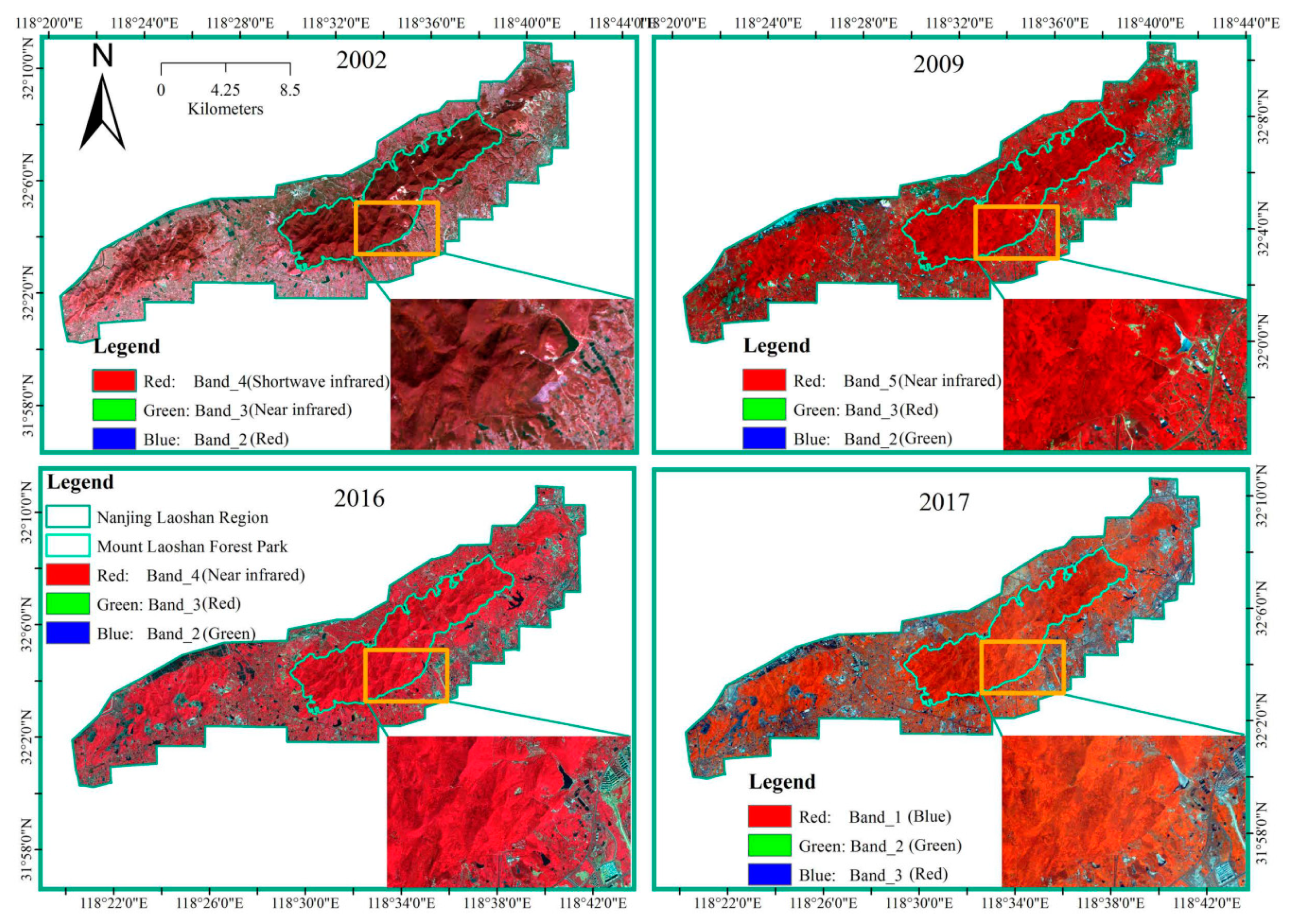
Orthorectified high-resolution imagery acquired by Satellite Pour l’Observation de la Terre (SPOT) in 2002 and 2016 and by Rapideye in 2009 and 2017 was used in this study (Table 1, Figure 2). The rational polynomial coefficient (RPC) orthorectification was processed for SPOT data and RapidEye data based on the NASA Shuttle Radar Topographic Mission (SRTM) digital elevation model (DEM) data. Then the rectified multi-spectral and panchromatic (pan) SPOT data were subjected to Gram-Schmidt Pan Sharpening for image fusion to get the panchromatic data’s high spatial resolution. The raw digital number values from the rectified RapidEye data were converted to top-of-atmosphere reflectance and then to do the FLAASH atmospheric correction. We then resampled them to 5 m with nearest neighbor interpolation to make the spatial resolution consistent for land cover mapping.

2.3. Land Cover Mapping (2002–2017) with Object-Oriented Classification

We implemented an object-oriented classification method combining image segmentation and SVM classification algorithms to identify four land cover types for the NLR, including urban, forest, cropland, and water. To implement the image segmentation, image composites were created by combining near infrared (NIR), red edge (RE), and red bands for the RapidEye data, and NIR, red, and green bands for the SPOT imagery. We then used a segment mean shift algorithm to generate image segments from the image composites [48]. This algorithm identifies image segments by grouping together adjacent pixels with similar spectral characteristics, based on averaged values calculated with a moving window for each pixel [48]. Segmentation parameters, including the spectral detail value, spatial detail value, and minimum segment size from Table 2, were used to generate the optimal segmentation objects and attributes. After image segmentation, we then applied the SVM algorithm to classify segmented objects based on the segment attributes (e.g., color, mean, standard deviation, count, etc.) into four land cover types with the training samples and DEM data. Sample polygons in the regions of interest (ROIs) for urban, forest, cropland, and water were collected on the segmentation objects referring to the Google Earth high resolution images (Table 2). All of the ROIs were extracted in locations where only a single land cover type covered the area.
The classification results were assessed with the random sampling strategy to perform classification accuracy assessment. We acquired the same number of points for all types that are used for classification (Table 2) from Google Earth imagery based on ground-truth data. We then generated the confusion matrix and calculated the overall accuracy and Kappa coefficient. The land cover products were then used as input data for the following steps in this study.

2.4. Land Covers Prediction Modeling

CA-Markov and STSM models represent two related but different land cover prediction techniques [28,34]. We applied both models in this study and compared their prediction capability to determine the optimal method for further steps. The CA-Markov model integrates CA’s capability of determining transition rules and simulating the spatial variation of every state in complex systems, and the Markov model’s advantage of making long-term predictions for future land cover trends (Figure S1) [33]. Here, we considered the dynamic changes in land cover as the Markov process. The cellular space refers to the land cover type map with its grid unit 5 m × 5 m as the cellular, the 5 × 5 adjacent grid pixels as neighboring cellular, and the four land cover types as four cellular states. The land cover type of the central cellular was determined using the transition rule based on the land cover type of the center cell and its adjacent grid cells at the previous moment (Figure S1). We then established a land cover transfer matrix, a state transfer probability matrix, and a transition suitability atlas based on the land cover maps for two dates using the Markov model. We selected a 5 × 5 mean contiguity filter in the CA model process. All of the predictions of the land cover changes with the CA-Markov model were processed in IDRISI software. Unlike CA-Markov model, the STSM algorithm is a spatially explicit approach to projecting landscape dynamics based on a stochastic process [35]. This algorithm represents space as a set of discrete spatial units, and time as discrete steps. The change in the discrete state of each spatial unit over time is modeled as a stochastic process and the time-inhomogeneous rates of change between states are expressed as probabilities [34]. Here, we defined the possible state types as the four land cover types identified in this study (Figure S2). We calculated the proportion of each transition type (Figure S2) based on the land cover maps generated in Section 2.3 from two dates. We then generated a transfer matrix to determine the transition probability of each type in the STSM model and set the probability within a similar distance to ensure the reliability of the simulation occurrence position. Finally, a predicted land cover map was derived. All of the simulations were conducted using ST-Sim (Version 3.1.2) in SyncroSim software (Version 2.0.3) [49]. Model inputs and outputs were prepared using the “rsyncrosim” package in R software (Version 3.3.1) [49].
To predict future land cover patterns, we first generated a land cover transfer matrix using the land cover maps created from 2002 to 2009 and from 2009 to 2016 in Section 2.3. We then applied both CA-Markov and STSM models to model the land cover types in 2016, 2018, and 2023 using a time interval of seven years. We further compared the CA-Markov and STSM modeling results in 2016 to identify the optimal method of land cover simulation. We assessed the overall accuracy and Kappa coefficients of the results based on the regions of interest (ROIs) for each land cover type (Table 2). We also assessed the spatial consistency of the simulation results from two models using a pixel-to-pixel matching method. This method overlays the simulated and observed maps and to spatially identify each spatial consistency or inconsistency pixel type. We compared the area and overall accuracy of spatially consistent and inconsistent regions between the predicted map and the 2016 land cover map generated in Section 2.3. The optimal predictive model was selected based on the accuracy and spatial consistency assessments, and then used to project the land cover patterns in 2018 and 2023 based on our mapping results from 2009 to 2016.

2.5. Spatial Analysis of Observed and Predicted Forest Cover Change

After developing the current and future land cover maps, we analyzed the spatial patterns of land cover change in our study from 2002 to 2023 with two objectives: (1) to examine the temporal rate of change for each land cover type; and (2) to quantify the current and future area of forest gain and loss in the NLR.
We then utilized a commonly used land use dynamic degree model to describe the change rate of land use types during a specific period. This model calculates the annual dynamic degree of land cover types using the following equation [50]:
K = [ ( U n + t U n ) U n ] × 1 T × 100 % ,
where K is the annual dynamic degree of one land use type over monitoring period time T, and Un and Un+t are the areas of this land use type at the beginning and end of period T, respectively [50]. A positive or negative K indicates a gain or loss in the spatial extent of one land use type. Abrupt, rapid, moderate, slow change, and no change were defined as >40%, 25–40%, 12–25%, 8–12%, and 0–7%, respectively [50].
We then applied the pattern-based morphological change detection (MCD) method to quantify the gain and loss area of forest cover [38]. This method captures the primary change area of loss and gain between two dates with morphological post-processing with three major steps (Figure S3): (1) identifying forest gain and loss polygons by overlaying the land cover maps; (2) determining areas with a high probability of change; and (3) reconstructing land cover change objects [38]. Using this method, we mapped the homogeneous and contiguous forest loss and gain during 7-year intervals from 2002 to 2023. We then calculated the areas of forest loss and gain as well as the annual deforestation rate. In particular, the annual deforestation rate was defined as follows [51]:
D R = 100 × [ 1 ( 1 F C t 2 F C t 1 F C t 1 ) ( 1 t 2 t 1 ) ] ,
where DR is the annual deforestation rate (in %/yr), FCt2 and FCt1 are the forest cover at both dates t2 and t1, respectively, and t2t1 is the time–interval (in years) between those two dates.

2.6. Fragmentation Analysis of the Forest Cover Change Pattern

After capturing the areas with primary forest loss and gain, we used FAD, a simple metric of fragmentation, as a contextual variable associated with a given forest pixel to analyze the fragmentation patterns in our study area. This metric is calculated as the percentage of forest pixels in a fixed-area neighborhood [44,52]. We calculated FAD at five measurement scales based on neighborhood sizes, including 7 pixels × 7 pixels (0.0008 km2), 13 pixels × 13 pixels (0.0028 km2), 27 pixels × 27 pixels (0.012 km2), 81 pixels × 81 pixels (0.108 km2), and 243 pixels × 243 pixels (0.969 km2), to characterize the forest fragmentation for the years of 2002, 2009, 2016, 2017, 2018, and 2023.
We then classified the FAD values into six classes, including rare (density <10%), patchy (≥10%), transitional (≥40%), dominant (≥60%), interior (≥90%), and intact (100%), to describe the fragmentation patterns (Table 3) [44]. Since our study area is relatively small, we re-defined the thresholds for the rare (<20%) and patchy (≥20%) classes. Different FAD ranges were then labeled as high (0–19%), medium (20–89%), and low (90–100%) fragmentation levels based on the FAD values within the neighborhood (Table 3).
A moving window size of 27 × 27 was selected to characterize the final level of forest fragmentation to balance between small and large neighborhoods, which is sensitive to fragmentation varying at a higher and lower spatial frequency, respectively [21]. The measurements were conducted using the function “r.neighbors” in the “rgrass7” R package [53]. We also compared the fragmentation pattern in 2009 generated in this study with other products developed with multi-source moderate resolution satellite imagery. Specifically, we considered the Phased Array L-band Synthetic Aperture Radar (PALSAR) on the Advanced Land Observing Satellite (ALOS)-based forest/non-forest (FNF) product in 2009 [54], and the 2010 forest/non-forest product developed from China’s 30 m global land cover (GlobeLand30, “GLC30”) dataset [55] (Table 4).
To estimate the change of interior and intact forest impact on fragmentation of the remaining forests, we calculated the ratio of the net percent change in loss of forest interior and intact area (FAD ≥ 0.9) divided by the net percent change in total forest area [13]. Larger positive ratio values indicate the forest interior and intact area loss has larger fragmenting effects on other forests, while the value is equal to 1, that is reversed [13].
We further compared the high-resolution pixels of forest loss and gain from 2002 to 2023 mapped with the MCD method, to understand the relationship between forest cover change (loss and gain) and fragmentation patterns (interior and intact regions, FAD ≥ 0.9) through the spatial analysis and statistical methods. The differences between gross gains and losses for FAD ≥ 0.9 represent the net changes of forest interior and intact area [11]. We intersected the forest loss pixels with the FAD ≥ 0.9 ones in 2002 to determine whether forest area losses were removing forest interior and intact area. We also intersected the forest gain pixels with the FAD ≥ 0.9 ones in 2023 to determine whether forest area gains were adding forest interior and intact area.

3. Results

3.1. Validation of Current and Future Land Cover Maps in the NLR

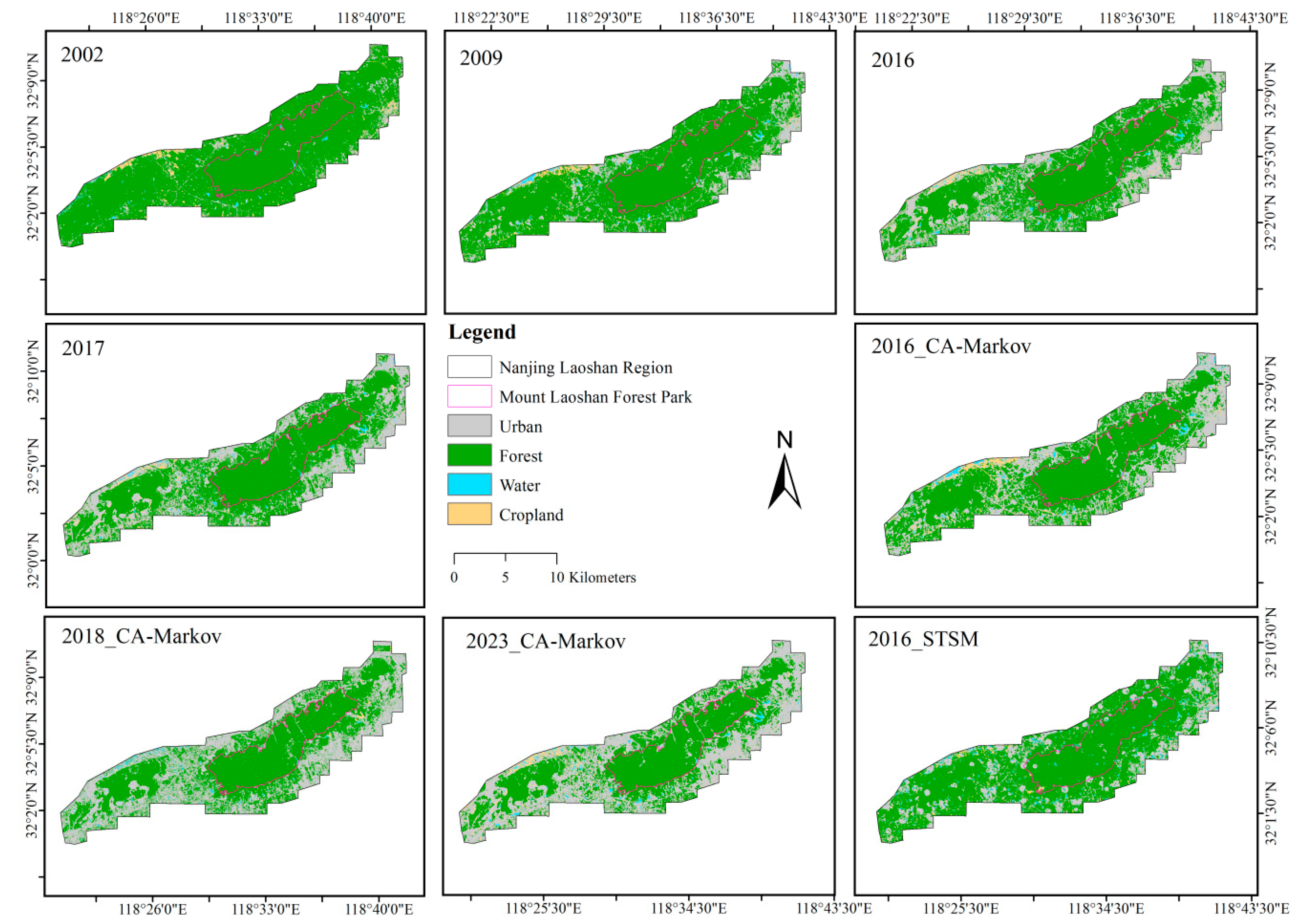
We summarized the accuracy assessment results of the RapidEye and SPOT-based land cover maps in 2002, 2009, 2016, and 2017 with selected ROIs (Table 5, Figure 3). The overall accuracy values were over 90% except for the year of 2002 (83.75%). The Kappa coefficient was over 0.78 for 2002 and reached up to 0.87–0.90 for the other years.
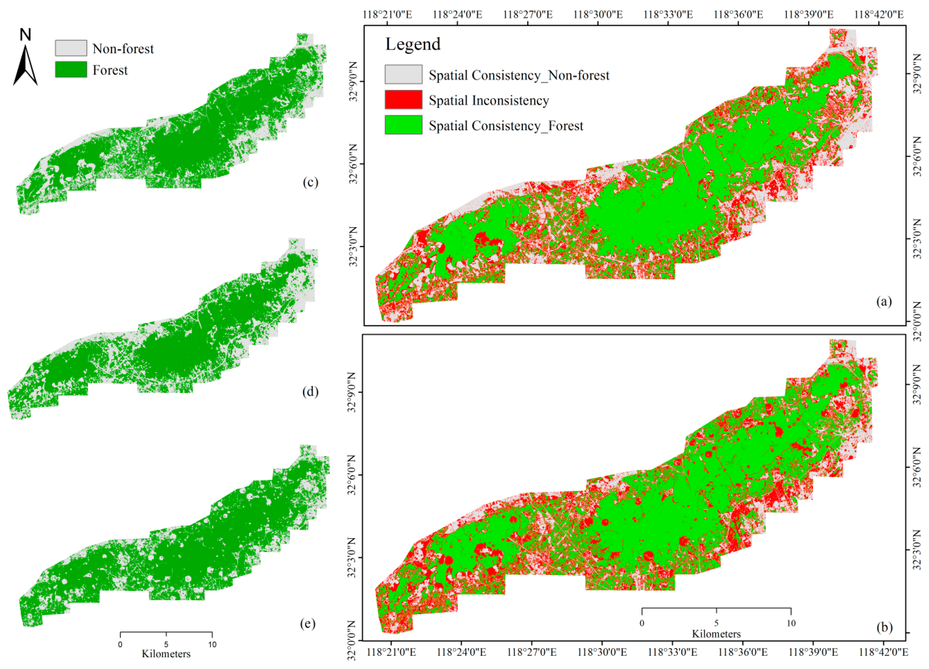
To assess the land cover prediction capability of the CA-Markov and STSM models, we first generated a confusion matrix for the simulated maps in 2016 with our selected ROIs (Table 5). The overall accuracy and Kappa coefficient based on the CA-Markov-based land cover map in 2016 reached 69.40% and 0.59, respectively, suggesting the superiority of the CA-Markov model over the STSM method (54.95% and 0.39, respectively). However, both methods were less accurate than the classification results derived from the 2016 SPOT imagery. We also examined the spatial consistency maps of the predicted 2016 map in comparison with the actual FNF map classified with SPOT imagery (Figure 4). The results of spatial consistency analysis show that the CA-Markov algorithm reached an overall accuracy of 76.14%, which was higher than the 73.53% accuracy of the STSM method. In addition, the STSM method identified a larger spatial inconsistent region (62.72 km2) than the CA-Markov method (56.50 km2). The spatial distribution of the predicted maps also suggests that the STSM results had more obvious noise (Figure 3 and Figure 4). Thus, the CA-Markov model was more effective than STSM in general and was identified as the optimal method for predicting land cover changes in the following steps (Figure 3).
The total forest area estimated from the SPOT-based land cover map in 2016 was 49.22 km2 for the MLFP (Figure 3), which was much lower than the 64 km2 recorded by the statistical data. The CA-Markov algorithm simulated the total forest park areas of 2016 and 2018 as 48.63 km2 and 48.45 km2, respectively; that of 2018 based on the CA-Markov algorithm was close to the land use planning data (46.55 km2, 91.9% of the total area; www.pukou.gov.cn).

3.2. Spatial Patterns of Current and Future Forest Cover Change in the NLR

3.2.1. Analysis of the Landscape Change Pattern

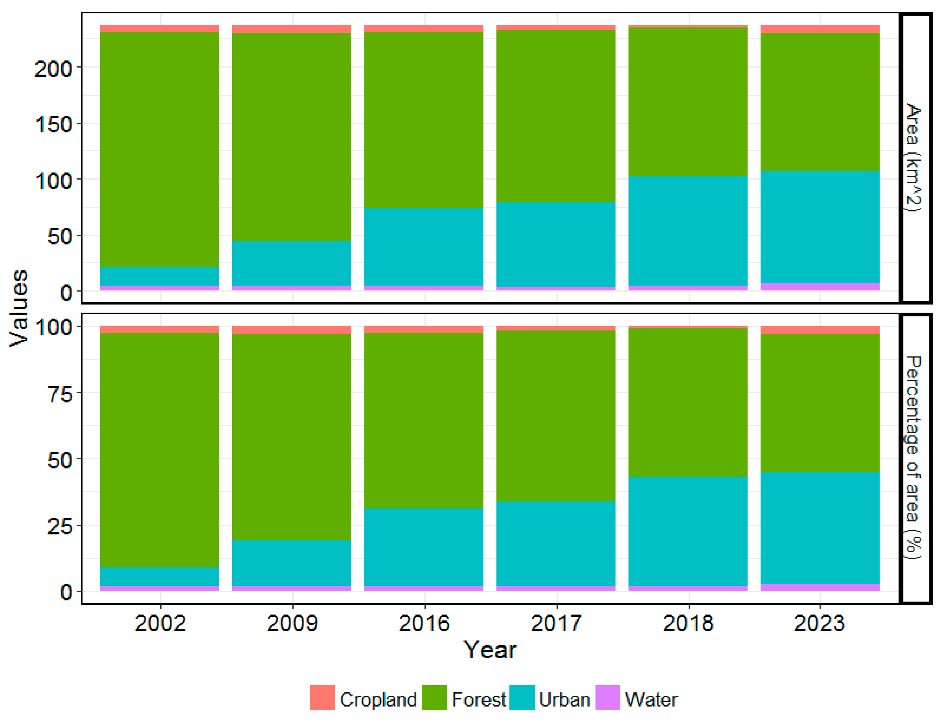
We summarized the total area and the percentage of area for each land cover type in our current and predicted land cover maps for multiple years (Figure 5). In general, we observed a gradually decreasing trend of forest area, while an increasing trend of urban, cropland, and water area. Specifically, we estimated a potential decrease of total forest area from 209.4 km2 to 123.9 km2 between 2002 and 2023 (40.8% decrease, about 52.3–88.4% of the total area). While we predicted about an 82.8% increase of the total urban area from 17.23 to 99.92 km2 between 2002 and 2023 (about 7.3–42.2% of the total area). The areas of cropland and water were relatively stable from 2002 to 2023, with slight increases of 8.7% and 35.2%, respectively.
Figure S4 shows the highest annual land use dynamic degree of the urban area among all four types, with 29.2% from 2002 to 2018 and 22.9% from 2002 to 2023. This also indicates a rapidly expanding trend of urbanization. The annual land use dynamic degree of forest remained stable with a prominent moderate negative change (−13.1%) from 2017 to 2018, indicating a loss of forest land. Moreover, the dynamic degree of cropland in land use exhibited abnormally negative values (cropland loss) from 2016 to 2017 and 2017 to 2018, as well as a positive value (cropland gain) from 2018 to 2023. Generally, the loss and gain of cropland were estimated to almost remain balanced during the period studied. The spatial extent of the water region tended to increase after 2017; this trend was evident from 2017 to 2018 with moderate change. In terms of the time intervals of every seven years, the urban region had a positive dynamic degree resulting in a gain in the area, but with a decreasing trend. Meanwhile, the water region showed a trend from no change that evolved to an increase. A negative dynamic of forest loss was constantly detected that did not change noticeably in the period.

3.2.2. Analysis of Forest Loss and Gain

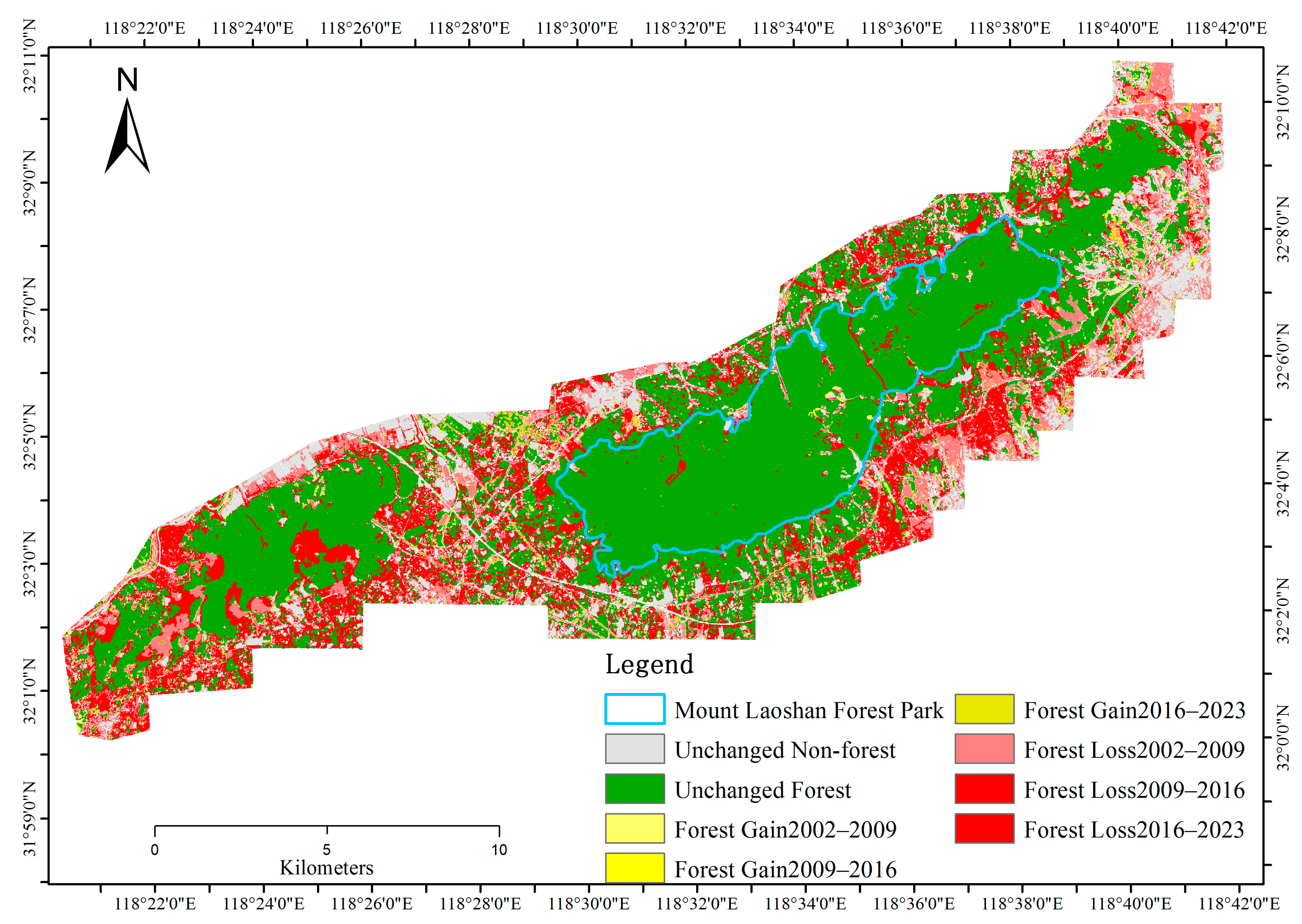
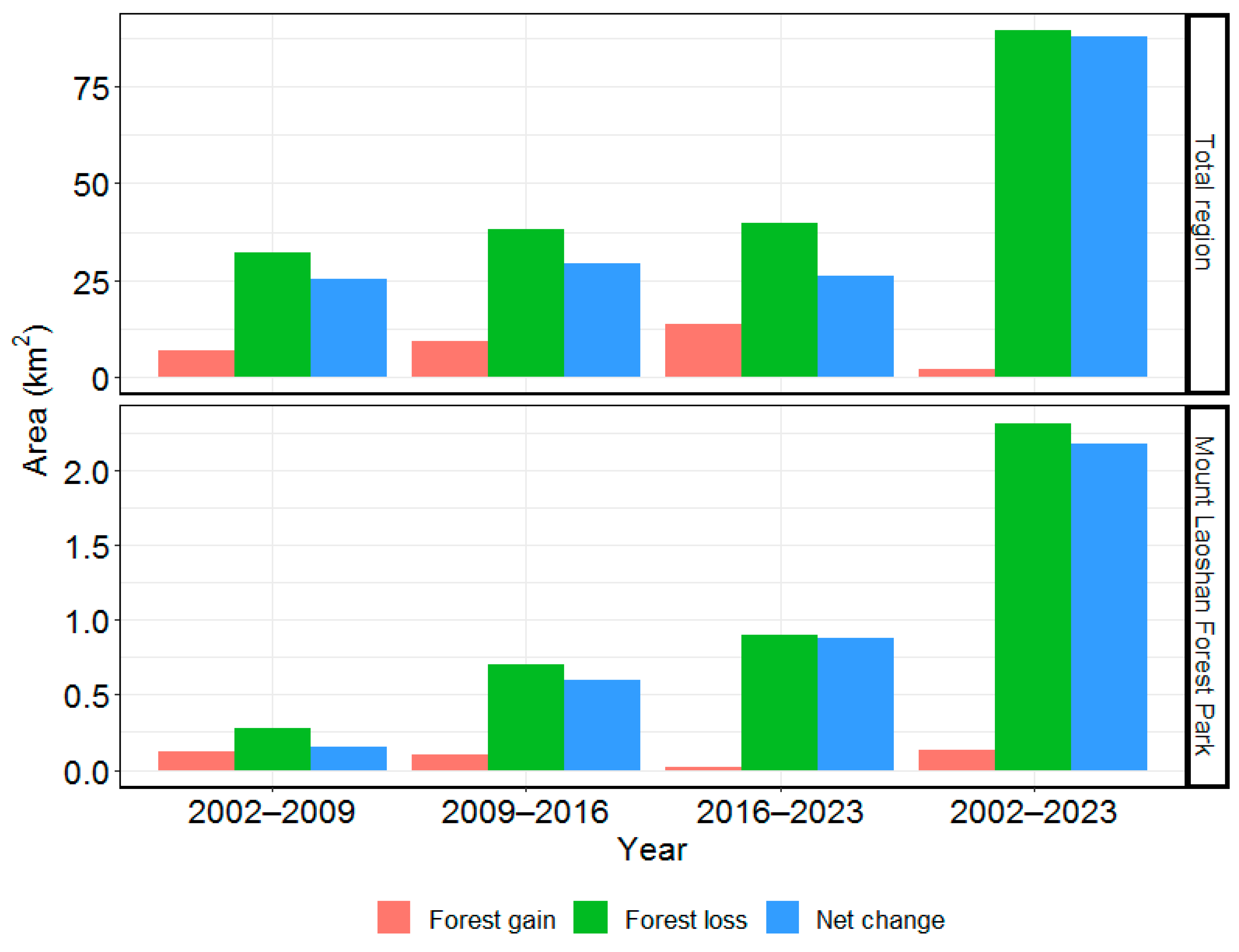
The forest cover change from 2002 to 2023 was mapped and summarized using the MCD method (Figure 6 and Figure 7). For the entire study area, the annual average forest loss and gain rates were about 4.27 km2 yr−1 and 0.09 km2 yr−1, respectively. In particular, the forest cover within the MLFP (Figure 6, blue solid line) had the smallest amount of relative gain (0.14 km2), loss (2.31 km2), and net change (2.18 km2) when compared to other land cover types. This forest cover change within the forest park was lower than its annual average amount for the entire study area, suggesting that the remaining region outside this park has experienced a massive forest loss (Figure 7). Generally, the rate of forest loss increased continuously over time, although some areas experienced forest gain; but the annual net positive change during the three time intervals was monitored with no marked changes along with a slightly higher value between 2009 and 2016 (29.2 km2; Figure 7). In the MLFP, continuous increases in forest loss and net change were found with a similar rising trend and had more than tripled over the period 2016–2023 (0.9 km2, 0.88 km2) compared to 2002–2009 (0.27 km2, 0.15 km2), respectively, while the opposite occurred with forest gain areas (0.02 km2, 0.12 km2; Figure 7).
A progressive increase in the deforestation rate by 4.07 km2 yr−1 (1.64% yr−1) was observed between 2002 and 2023 (Table 6). For the three time intervals, the deforestation rate progressively increased from 3.45 km2 yr−1 (1.57% yr−1) during the period 2002–2009 to 4.75 km2 yr−1 (2.78% yr−1) during the period 2016–2023 (Table 6). The smallest deforestation rate was detected from 2018 to 2023 (1.85 km2 yr−1 or 1.35% yr−1). From 2016 to 2017, we calculated a high deforestation rate (4.01 km2 yr−1, 2.6% yr−1), which was followed by that during 2016–2023, but was greater than that of the period 2018–2023, indicating a noticeable increase of deforestation occurred between 2016 and 2018 (Table 6).

3.3. Analysis and Variation of the FAD-Based Forest Fragmentation Data

3.3.1. FAD-Based Forest Fragmentation Data and its Variability

Five moving window neighborhood sizes were chosen to calculate and map FAD-based forest fragmentation (Figure S5). The change in forest fragmentation was not very obvious after 2002 after reviewing all of the window sizes; however, the change trend of the low and highly fragmented forest was consistent (Figure 8 and Figure S5). The area of forest with limited fragmentation had a general decreasing trend since 2002, with a small increase from 2018 to 2023. The area of highly fragmented forest remained relatively stable with no obvious dynamic change; only a slight difference was observed in and after 2018, especially in 2018. The forest area with a medium level of fragmentation initially increased and then decreased over time. The area of forest pixels belonging to the forests with a low level of fragmentation was at least 40 times greater than that of highly fragmented forest.
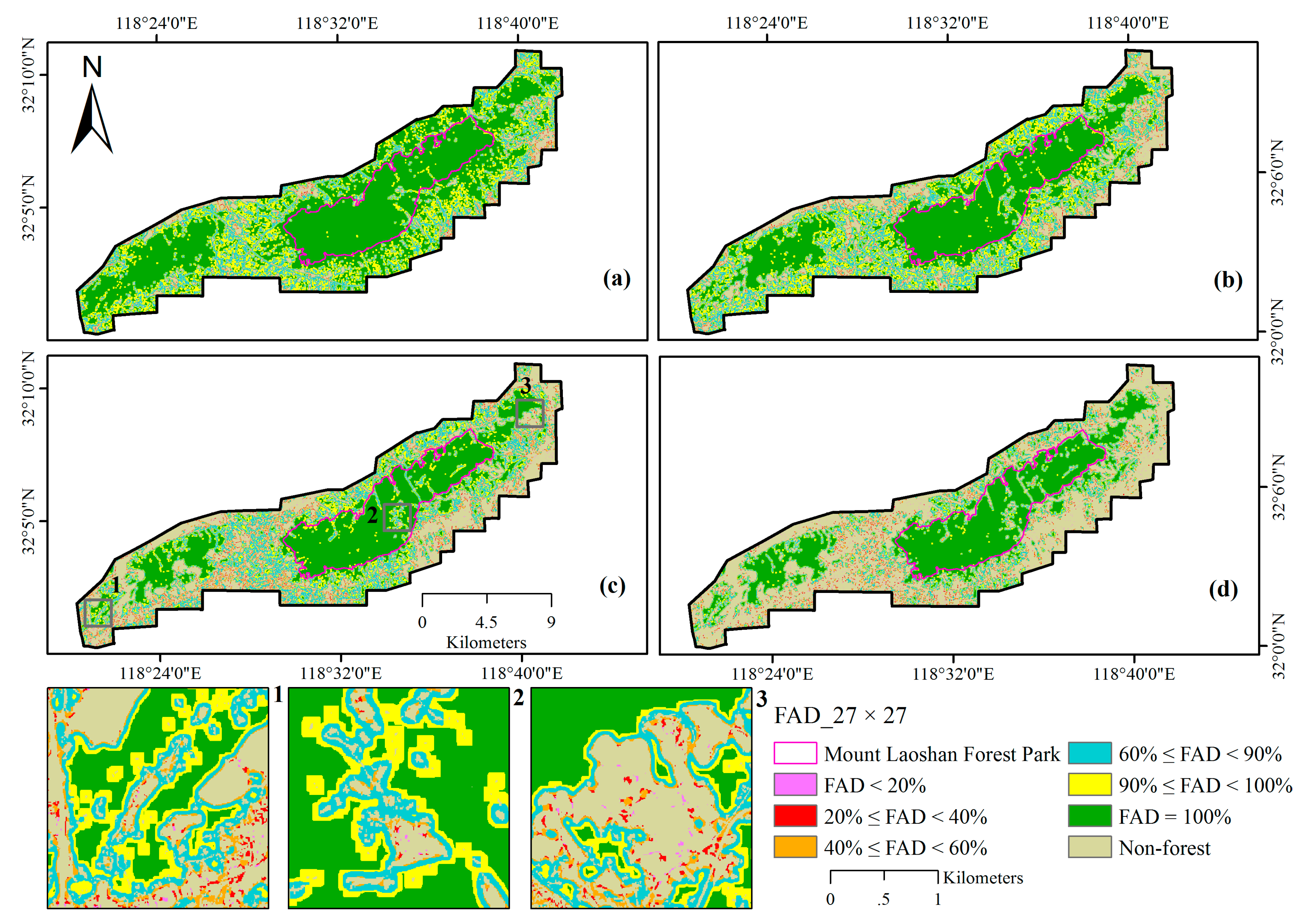
Figure 9 shows the measurement results of FAD based on the neighborhood size of 27 × 27 that was selected as a compromise in 2002, 2009, 2016, and 2023 as discussed below. We reported that forests with a limited level of fragmentation accounted for the highest proportion of all of the fragmentation classes, while the percentage of forest belonging to the highly fragmented forest was relatively low from the main region map and three enlarged maps. Most region of MLFP has limited fragmented in a high percentage of its forests. Additionally, the highly fragmented region was usually far from the forest interior regions based on visual judgment. In summary, the area with no forest fragmentation decreased with some variation, especially in the western part of the entire region after 2016 (Figure 9c). Meanwhile, there was an evident but not dramatic trend towards fragmentation in MLFP. The forest areas with a low level of fragmentation were gradually being transferred to forest approaching a high level of fragmentation, most of which mainly occurred outside MLFP.
Based on the selected window size of 27 × 27, the percentage of highly fragmented forest has increased from 0.1% in 2002 to 3.1% in 2018 and then decreased to 1.4% in 2023 (Table 7). Overall, at least half of all of the forests had limited fragmentation with some variation. The decreasing trend of the percentage of forest belonged to the two forest classes with limited fragmentation (FAD ≥ 90%) decreased from 81.1% in 2002 to 64.1% in 2023, with a slight peak in 2017 (Table 7). In 2016, 62.9% of the forest had a limited level of fragmentation while only 0.7% of the forest was highly fragmented. However, by 2018, these percentages had changed to 59.6% and 3.1%, respectively. In 2023, the amount of highly fragmented forest was predicted to moderate, but the percentage was consistently higher than before 2018; moreover, the percentage of the forest interior region was lowest (12.1%) and remained consistent with that in 2018. Unfragmented (intact, FAD = 1) forest recovered in 2023 with the percentage (53.3%) being close to that in 2002 (57.4%, Table 7).

3.3.2. Detecting and Quantifying Changes of Forest Fragmentation

Table S1 shows the relative contribution of each fragmentation class change separated for each type of change fraction and increase and decrease in fragmentation. Considering the internal change of the interior and intact class, a gross fragmentation decrease was found of 7.9%, 11.3%, and 1.0% for the sequence of three 7-year time intervals between 2002 and 2023, respectively. Excluding the changes between interior and intact forests, 54.6%, 55.7%, 53.8%, and 68.9% of all of the fragmentation increase was calculated for interior and intact transferring to other classes; meanwhile 46.3%, 44.8%, 49.8%, and 34.0% of all fragmentation decrease was found for other class transferring to interior and intact during 2002–2009, 2009–2016, 2016–2023, and 2002–2023, respectively, leading to a gross forest fragmentation increase of 8.3%, 10.9%, 4.0%, and 34.9%, respectively. Overall, we summarized a net fragmentation change trend of an initial increase followed by a decrease during three time intervals (2002–2023) among the changes between intact (i.e., no fragmented forest) and other classes (i.e., fragmented forest); the greatest fragmentation increase (3%) was detected between 2016 and 2023, and the greatest fragmentation decrease (0.4%) was between 2009 and 2016.

3.3.3. Estimation of the Multi-Source Data Impacts on Forest Fragmentation

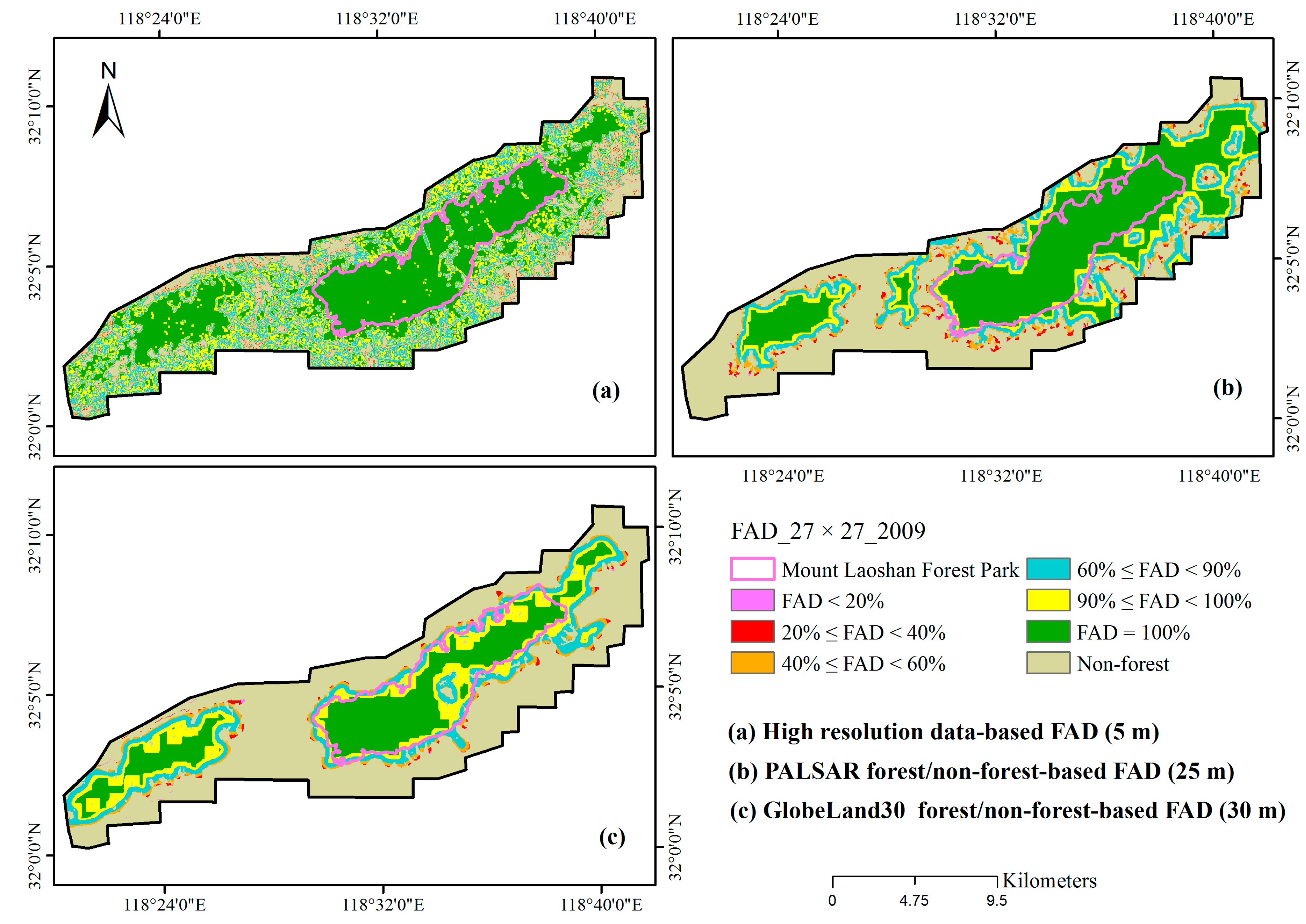
We applied three datasets to derive the 27 × 27 window size-based fragmentation spatial patterns in 2009 (Figure 10). High resolution data can detect finer levels of forest and fragmentation details than coarse resolution products (Figure 10). For the MLFP, the majority of intact forest (FAD = 1) could be detected along with non-apparent interior forest (90% ≤ FAD < 1) and other levels of forest fragmentation in Figure 10a. While most of intact forest and the largest area of forest can be found in Figure 10b, and an obvious intact and interior forest and the least area of forest were found in Figure 10c.
In addition, the high resolution RapidEye 5 m land cover data allowed the identification of the largest forest cover of about 185 km2, followed by the PALSAR 25 m forest/non-forest product (144 km2), and the China’s 30 m global land cover product (109 km2). Meanwhile, the area of interior and intact forest had the same patterns among these three products.
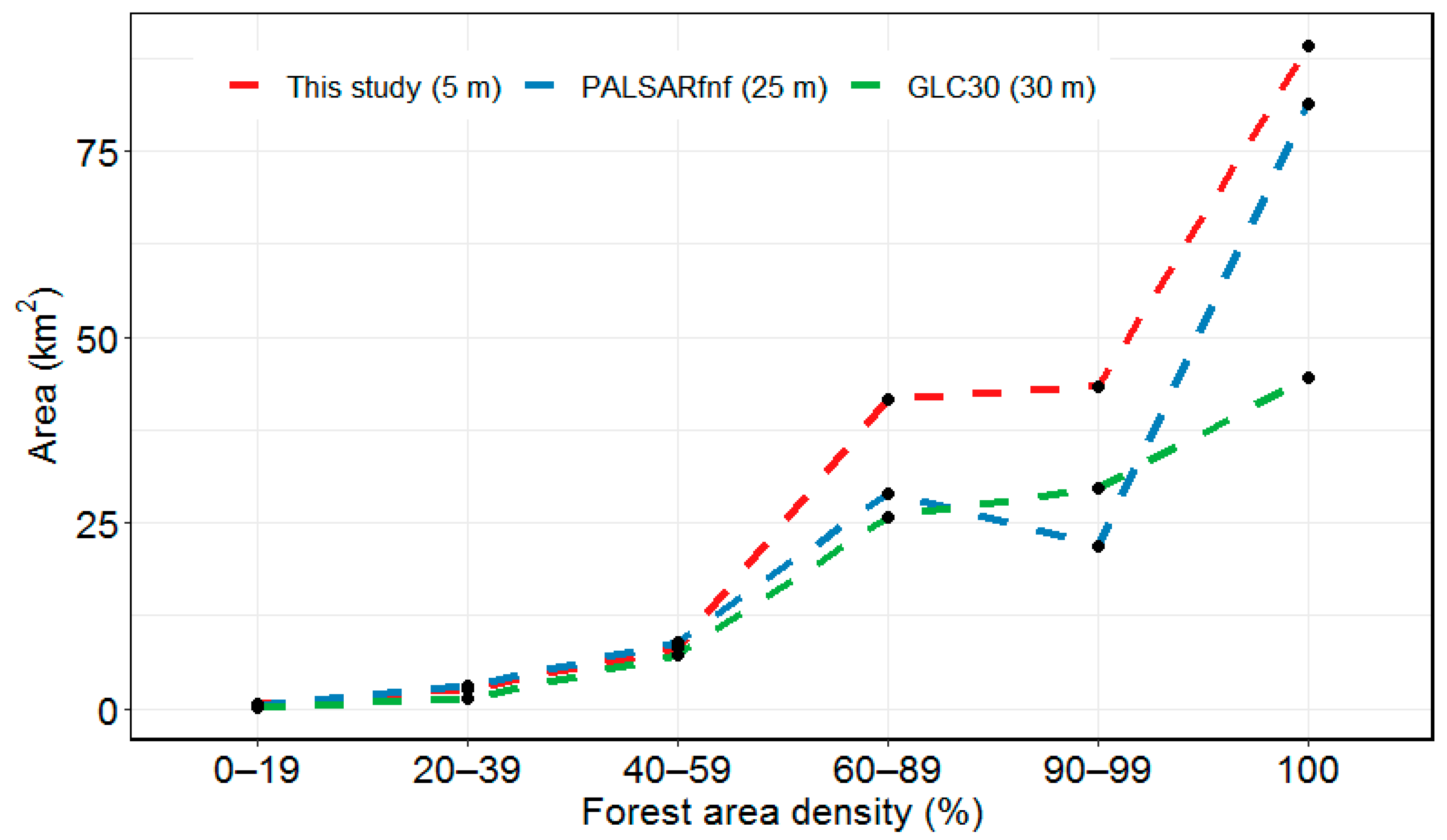
Moreover, this discussion uses the FAD classes generated with the three data sources and defined in Table 3. Figure 11 shows that an overall increasing trend for the area of forest fragmentation from rare forest (0–19%, <1 km2) to intact forest (100%), particularly with the high resolution data. The substantial amounts of rare forest (0–19%), dominant forest (60–89%), interior forest (90–99%), and intact forest (100%) characterized by the high resolution land cover data were identified, especially for dominant and interior forest, which were approximately twice greater than the data from medium resolution PALSAR and Landsat-based land cover data (Figure 11). Naturally but unexpectedly, the amount of intact forest identified by the GLC30 (44.5 km2) was less than half of that found in this study (89.19 km2) accompanied by the area of 81.31 km2 found using the PALSAR data. Overall, the estimates of the area of dominant, interior, and intact forest (particularly the first two) by the high-resolution data exceeded their medium resolution counterparts.

3.4. Evaluation of Forest Fragmentation Dynamics Associated with Forest Changes

The loss rate of forest interior and intact area shows an increasing trend during the three time periods (Table 8). A greater increasing trend in the first two time periods between 2002 and 2009 and 2009 and 2016 than the latter periods between 2009 and 2016 and 2016 and 2023 was observed. The net decreasing rate for area of interior and intact forest was larger than the rate of total forest loss, but with a little difference, and leading to their positive ratio (Table 8). From 2002 to 2023, the decreasing rate in the spatial extent of interior and intact forest was estimated as 43.44%, which was higher than the 41.95% of the total forest area, but with the lowest ratio of 1.04. The 2002–2009 period had the greatest ratio of 1.17 among all time periods (Table 8). Hence, although a greater net decrease rate of forest interior and intact area than that of the total forest area was generated, the ratio among all time periods was nearly equal to 1, suggesting that forest interior and intact area loss had slight fragmentation effects on other forests.
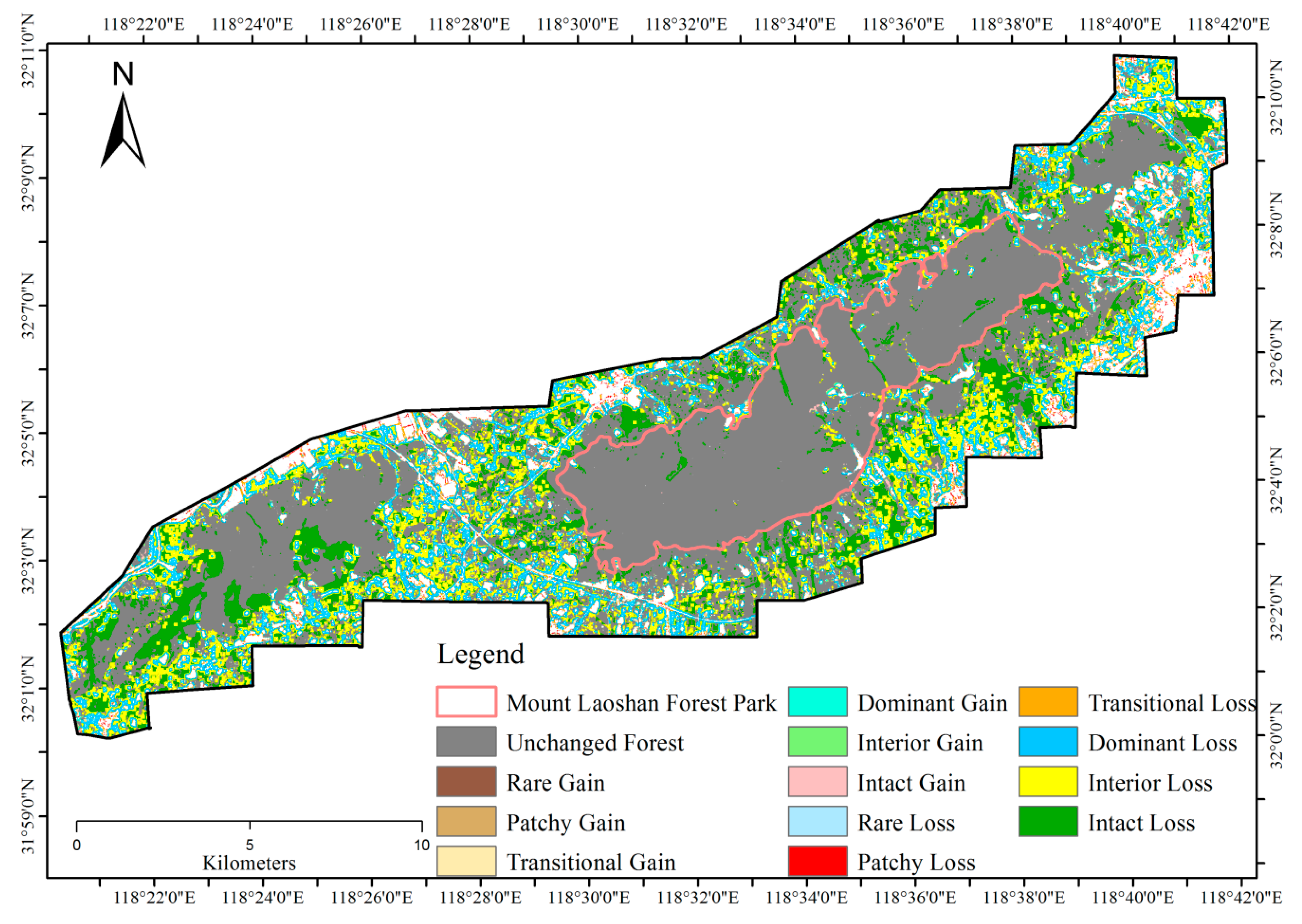
Figure 12 illustrates the spatial pattern of forest loss and gain in relation to the forest fragmentation region from 2002 to 2023. We found that forest area losses were removing 58.07 km2 of forest interior and intact area, which was approximately twice that of other fragmented forests. Meanwhile, forest area gains were adding 0.35 km2 of forest interior and intact area, which was a fourth lower than that of other fragmented forests. Net forest loss in relation to forest interior and intact area (by 57.73 km2) was approximately twice greater than other fragmented forests (by 29.58 km2). We found a large area forest loss from intact and interior forest in the western forests of this study area, which was especially true for loss from intact forest. Although no obvious change was detected in the MLFP, there was a conspicuous forest loss from intact and interior forest in the southern part near the park.

4. Discussion

4.1. Mapping Spatiotemporal Dynamics of Current and Future Forest Cover

This study demonstrated the effectiveness of using high-resolution remote sensing imagery with RapidEye and SPOT data for urban land cover mapping in the NLR of China, with an overall accuracy of more than 90%. Our results suggest that RapidEye data can contribute to urban forest monitoring by incorporating the RE band, which is sensitive to detecting vegetation based on the chlorophyll reflectance of absorbing wavelengths [56,57]. We also show the strong capability of object-oriented classification using a support vector machine (SVM), which has been found superior to classifiers such as classification and regression trees and K nearest neighbor in existing research [58]. Recent studies have also suggested that the popularity of object-oriented classification with random forest has the best performance, and could be applied in future work [59].
Using the CA-Markov and STSM algorithms, we found overall accuracy values of 69.40% and 54.95% and Kappa coefficients of 0.59 and 0.39 of the 2016 predicted land cover maps, respectively. Meanwhile, the CA-Markov-based method did not exceed the standard acceptable accuracy (85%) [28]. Nevertheless, it had reasonable consistency values (above 0.4) between two images based on Kappa values compared to STSM, although the results were not substantial and perfect [30]. Excluding the function of the prediction models, the accuracy of the existing land cover maps in 2002 and 2009 were found to entirely determine the predicted map in 2016, but a slightly lower overall accuracy of 83.75% was found in 2002 (Table 5); therefore, double errors from the two processes by classification and prediction may result in an unreasonable level of accuracy [28]. Moreover, the mis-registration of the two overlaying maps from 2002 and 2009 could lead to significant errors in our final results of predictive modeling or spatial overly consistency analysis [60]. Overall, the key point was the reasonable selection of the first two images [28]. Hence, it does not directly mean the validation and spatial consistency accuracy of the prediction maps in 2018 and 2023 will be lower than in 2016, because the accuracies of the first two years-based land change dynamics above 90% will reduce the errors of the change detection from classification. In addition, the parameters setting and the insufficient consideration of the driving factors (e.g., ecological damage, protection, and restoration, as well as urbanization) affecting land cover change during different time periods would affect the simulating process and accuracy [30].
The overall accuracy assessment (Table 5) and spatial distribution of predicted land cover map for 2016 (Figure 4) suggest that CA-Markov modeling is superior to STSM in our study area. Compared to STSM, the CA-Markov algorithm integrates the advantages of both cellular automata (CA) and Markov chain. However, STSM can be considered a type of Markov chain; it is possible to observe a salt and pepper effect in the output image from the Markov procedure, which can limit the performance of the STSM algorithm [35]. Furthermore, developing forest cover maps with high spatiotemporal resolution for small regions such as NLR is still challenging because of the limited availability of imagery [26].

4.2. Assessment of Forest Cover Change Detection Methods

In general, the forest type continues to dominate the study area but a long term decreasing trend was observed, while the deforestation rate or urbanization have increased rapidly especially since 2016. This could be explained by the establishment of NJNA in 2015 with urbanization and infrastructure construction continuing (www.najing.gov.cn). Additionally, this region has a mining area that was abandoned before 2000, leading to the complete removal of vegetation. This can be easily identified in the National Statistical Yearbook although high-resolution imagery is lacking for that time period. Some plantation forest and landscape reconstruction strategies have been adopted resulting in some forest recovery since 2002 (Figure S6). Nevertheless, this might not function as a permanent solution for mine revegetation and recovery for these abandoned areas, because a decreased in forest cover was found in mining areas since 2011 (Figure S6).
Moreover, the trend of annual land use dynamic degrees of all of the land cover types reached agreement with the change of the area from 2002 to 2023. However, regional differences in land use characteristics were also found with the dynamic degree in annual monitoring period [50]. The cropland loss that experienced rapid and abrupt change in 2016–2017 and 2017–2018, and abrupt gain simulated for 2018–2023 may be caused by errors in the predicted land cover data such as the confusion between bare land and cropland in 2018, although this does not affect the calculation of forest loss and gain with the binary forest/non-forest data [38].
Conservation and planning strategies for MLFP have been adopted (www.najing.gov.cn). Yet the overall trend of the planning area and land use from 2018 to 2027 (www.pukou.gov.cn) was inconsistent with the predictions for 2018–2023 (Figure 6), especially for forests and croplands. Although model prediction results as a reference might have some uncertainties, it is necessary for policy makers to avoid deforestation and degradation practices and they need to implement the conversion of cropland to forests rather than to consider urbanization and construction in the future (www.pukou.gov.cn).

4.3. Assessment of Variations in Forest Fragmentation over Time

Existing studies have suggested that pixel size of land cover data or spatial scales can lead to different results during fragmentation analysis. For example, Ritters et al. [21] found that a smaller pixel size or high resolution data-based fragmentation analysis would not show more fragmentation when compared with larger pixel or lower resolution data. However, other studies indicate that high resolution data could detect more detailed anthropogenic fragmentation [61], or larger contagious forest cover even at larger spatial scales [25]. It seems that choosing an appropriate scale of 27 × 27 with high resolution data at 5 m was reasonable and useful. This data-based technique showing the identification of the highest forest area was consistent with the results from Wickham and Ritters [25]. However, the former high resolution-based technique had detected more dominant, interior, and intact forest than the medium resolution data due to the high uncertainties in identifying low density disturbances [62]; nevertheless, the latter had lower estimates of intact forest when compared with the high resolution data [25]. Otherwise, GLC30-based results had a trend that was inconsistent with those from the other data resolution sizes, especially for intact forest, because GLC30 was acquired starting from 2010. Ultimately, shifting from coarse or medium resolution sources to high resolution image sources is inevitable [25].
A continuous expansion of human land-use would lead to further land degradation, create highly fragmented zones, and impact the interior forest; however, the opposite issue can been seen in Figure 9 [7,61]. Usually, protecting transitional and adjacent areas might limit expansion or degradation of the transitional areas; the condition of forests with limited fragmentation appears to transfer to highly fragmented forests and was consistent with the effect of protective measures in the NLR [61]. A lack of control efforts on the degree of expansion could cause high levels of fragmentation, such as the effects on the interior forests caused by expansion of the NJNA in 2016 (Table 7 and Table S1). Additionally, either ecological restoration or mining restoration were adopted between 2009 and 2016 and add to the existing forest area (Table S1), but these efforts to not mean a rapid elimination or reduction in fragmentation, because these restoration efforts may not produce larger patches of interior forest because the total forest area has already decreased (Figure 9, Table 7) [63]. Wader et al. [61] considered that having the greatest amount of intact forest was easy to achieve even with high levels of fragmentation in South Africa. In general, forest protection and restoration measures taken by the policymakers devoted to managing the NJNA have restored the interior forest, especially the intact forest from 2018–2023 in MLFP (Figure 9, Table 7) (www.pukou.gov.cn). Hence, having a large area of intact forest is extremely important when eliminating or reducing any current or future human-caused fragmentation, such as between 2016 and 2023 (Table S1) [1,11,15,64].

4.4. Forest Cover Change and Effects on Forest Fragmentation

The transitions between forest fragmentation classes could be explained by forest loss and gain in our study [11]. Although the majority of forest area loss can be found in what was previously interior forest, most forest area gain was not sufficient to add interior forest (Figure 12). This discovery was consistent with that of Ritters and Wickham [11] and Ritters and Costanza [15]. Since the forest interior and intact loss area was greater than total forest loss area, we suggest that forest interior patterns could be more suitable for understanding the effects of human activities [11]. Most forest area loss was from interior and intact forests (Figure 12), but few effects were found on other remaining forests (Table 8) depending on the direct conversion of forest interior to non-forest area, such as that caused by urbanization and infrastructure, which occurs at a certain distance from the forest edge land type [13]. Otherwise, loss of the restored forests in the mining area concentrating in the western part of the study region had a slight influence on the remaining area when compared to the entire area, because conservation and restoration measures may improve the connectivity of interior forest (Figure 12) [41]. Moreover, several studies have proved that increasing forest cover may not necessarily lead to a more homogenous forested landscape, and may trigger increasing or decreasing forest fragmentation, depending on the rate, extent, and causes of the increase in forest cover such as land-ownership and land-use legacy patterns [15,63]. Since forest gain follows mining activities, harvesting or land abandonment is a slow and gradual process (Figure S6) [65], incorporating spatial data covering a long time period such as 50 years or more from the historical era to the future rather than merely considering 20 years as important to capturing the effects of increases of forest cover on forest fragmentation [63].

4.5. Uncertainties and Future Work

The present study focused on urban forests in the NLR, which represents only a small portion of the entire NJNA. Our findings in the Laoshan Region likely differ from the results for the entire NJNA, due to the variability in topographic, social, and economic factors [47]. Although forest cover maps developed with high-resolution remote sensing imagery with intrinsic differences between image capturing sensors and external differences in model parameter settings and driving factors might improve the accuracy of fragmentation mapping [25,30,40,66], multi-sources, temporal data, and algorithms, including LiDAR, advanced mapping models, in situ inventories, and biodiversity data are required to enhance our understanding of the causes and consequences of forest fragmentation [19,47,66,67]. Nevertheless, monitoring the abrupt changes in forest interior, especially for intact forest, can assist effective conservation efforts in urban forest ecosystems [12,68,69].

5. Conclusions

In this work, we proposed a method to understand the relationship between forest cover change and forest fragmentation in the Nanjing Laoshan Region of Jiangsu, China from 2002 to 2023. We integrated object-oriented classification and landscape modeling to derive current and future forest cover maps based on high-resolution remote sensing data. Our results demonstrated the capability of high-resolution land cover products to identify detailed forest change patterns. We then explored the forest cover change with the MCD method and fragmentation pattern based on the FAD to examine the effects of forest changes on interior and intact forests. We identified a decreasing trend of forest area and net forest area loss related to the interior and intact forests. We also found a slight fragmentation effect of forest change on the remaining regional forests, indicating the overestimation of ecological risks from the loss of forest interior and intact region, caused by the protection and restoration of interior forests. Although challenges exist for examining the effects of urban forest change on fragmentation when combining satellite observations and in situ measurements, this sustained task in exploring forest interior and the forest itself is critical to providing sustainable management guidance for rapidly changing urban forest regions.

Supplementary Materials

The following are available online at https://www.mdpi.com/2072-4292/12/1/155/s1, Figure S1: Workflow of the CA-Markov model for land cover prediction in 2016, 2017, and 2023, Figure S2: The state-and-transition simulation model (STSM) of LULC change, where the boxes represent states and the arrows represent transitions, Figure S3: The workflow of morphological change detection (MCD) referred to Seebach et al. 2013, Figure S4: Annual land use dynamic degree of four land cover types during the period 2002–2023, Figure S5: Change in forest fragmentation during 2002 to 2023 calculated by 5 spatial scales defined by neighborhood size (7 × 7, 13 × 13, 27 × 27, 81 × 81, and 243 × 243, respectively) in Nanjing Laoshan Region, Jiangsu, China. FAD, forest area density, Figure S6: Forest recovery has been shown in and after 2002 and forest decreasing has been shown from 2011 in the typical mining abandoned areas. The first two photos represented two image composites by combining green, red, and near infrared for SPOT 5 in 2002 and blue, green, and red for RapidEye in 2009, respectively. The other photos in 2008, 2011, 2016, and 2019 were acquired from Google EarthTM, Table S1: Transition matrix of relative changes in forest fragmentation classes for 27 × 27 during 2002–2009, 2009–2016, 2016–2023, and 2002–2023. Fragmentation increase is found below the matrix diagonal with positive percentages and fragmentation above the matrix diagonal with negative percentages. Zero is equivalent to no change.

Author Contributions

W.S. designed the study, analyzed the data and wrote the paper. M.L. and C.H. helped in project design, paper writing and analysis. J.H. and J.D. helped in paper review and editing. X.M. helped in the original data preparation and data analysis. All authors have read and agreed to the published version of the manuscript.

Funding

This work was jointly supported by the Natural Science Foundation of China [31971577, 31670552], China Postdoctoral Science Foundation [2019M651842], and the Priority Academic Program Development of Jiangsu Higher Education Institutions (PAPD). Additionally, this work was performed while the first author was funded by the 2019 Postdoctoral Fellowships of Jiangsu Province, and the corresponding author acted as an awardee of the 2017 Qinglan project sponsored by Jiangsu Province.

Acknowledgments

The anonymous reviewers’ comments and suggestions greatly improved our paper. We are grateful for their kind help. Special thanks need to go to the Nanjing Pukou Forestry Station for providing local materials. We also thank Miss Qian Chen in provision of the aid of the data preparation.

Conflicts of Interest

No potential conflict of interest was reported by the authors.

References

  1. Betts, M.G.; Wolf, C.; Ripple, W.J.; Phalan, B.; Millers, K.A.; Duarte, A.; Butchart, S.H.M.; Levi, T. Global forest loss disproportionately erodes biodiversity in intact landscapes. Nature 2017, 547, 441–444. [Google Scholar] [CrossRef] [PubMed]
  2. Liu, J.; Coomes, D.A.; Gibson, L.; Hu, G.; Liu, J.; Luo, Y.; Wu, C.; Yu, M. Forest fragmentation in China and its effect on biodiversity. Biol. Rev. 2019, 94, 1636–1657. [Google Scholar] [CrossRef] [PubMed]
  3. Gong, C.; Yu, S.; Joesting, H.; Chen, J. Determining socioeconomic drivers of urban forest fragmentation with historical remote sensing images. Landsc. Urban Plan 2013, 117, 57–65. [Google Scholar] [CrossRef]
  4. Kupfer, J.A. National assessments of forest fragmentation in the US. Glob. Environ. Chang. 2006, 16, 73–82. [Google Scholar] [CrossRef]
  5. MacDonald, K.; Rudel, T.K. Sprawl and forest cover: What is the relationship? Appl. Geogr. 2005, 25, 67–79. [Google Scholar] [CrossRef]
  6. Chazdon, R.L. Beyond deforestation: Restoring forests and ecosystem services on degraded lands. Science 2008, 320, 1458–1460. [Google Scholar] [CrossRef] [Green Version]
  7. McIntyre, S.; Hobbs, R. A framework for conceptualizing human effects on landscapes and its relevance to management and research models. Conserv. Biol. 1999, 13, 1282–1292. [Google Scholar] [CrossRef]
  8. Wickham, J.D.; Riitters, K.H.; Wade, T.G.; Coan, M.; Homer, C. The effect of Appalachian mountaintop mining on interior forest. Landsc. Ecol. 2007, 22, 179–187. [Google Scholar] [CrossRef]
  9. Saunders, D.A.; Hobbs, R.J.; Margules, C.R. Biological consequences of ecosystem fragmentation: A review. Conserv. Biol. 1991, 5, 18–32. [Google Scholar] [CrossRef]
  10. Laurance, W.F. Theory meets reality: How habitat fragmentation research has transcended island biogeographic theory. Biol. Conserv. 2008, 141, 1731–1744. [Google Scholar] [CrossRef]
  11. Riitters, K.H.; Wickham, J.D. Decline of forest interior conditions in the conterminous United States. Sci. Rep. 2012, 2, 653. [Google Scholar] [CrossRef] [PubMed] [Green Version]
  12. Watson, J.E.M.; Evans, T.; Venter, O.; Williams, B.; Tulloch, A.; Stewart, C.; Thompson, I.; Ray, J.C.; Murray, K.; Salazar, A.; et al. The exceptional value of intact forest ecosystems. Nat. Ecol. Evol. 2018, 2, 599–610. [Google Scholar] [CrossRef] [PubMed]
  13. Riitters, K.; Wickham, J.; Costanza, J.K.; Vogt, P. A global evaluation of forest interior area dynamics using tree cover data from 2000 to 2012. Landsc. Ecol. 2016, 31, 137–148. [Google Scholar] [CrossRef] [Green Version]
  14. Wickham, J.D.; Riitters, K.H.; Wade, T.G.; Homer, C. Temporal change in fragmentation of continental US forests. Landsc. Ecol. 2008, 23, 891–898. [Google Scholar] [CrossRef]
  15. Riitters, K.; Costanza, J. The landscape context of family forests in the United States: Anthropogenic interfaces and forest fragmentation from 2001 to 2011. Landsc. Urban Plan 2019, 188, 64–71. [Google Scholar] [CrossRef]
  16. Skole, D.; Tucker, C. Tropical deforestation and habitat fragmentation in the Amazon: Satellite data from 1978 to 1988. Science 1993, 260, 1905–1910. [Google Scholar] [CrossRef] [Green Version]
  17. Davis, C.H.; Wang, X. Planimetric accuracy of Ikonos 1 m panchromatic orthoimage products and their utility for local government GIS basemap applications. Int. J. Remote Sens. 2010, 24, 4267–4288. [Google Scholar] [CrossRef]
  18. Myint, S.W.; Gober, P.; Brazel, A.; Grossman-Clarke, S.; Weng, Q. Per-pixel vs. Object-based classification of urban land cover extraction using high spatial resolution imagery. Remote Sens. Environ. 2011, 115, 1145–1161. [Google Scholar] [CrossRef]
  19. Hermosilla, T.; Wulder, M.A.; White, J.C.; Coops, N.C.; Pickell, P.D.; Bolton, D.K. Impact of time on interpretations of forest fragmentation: Three-decades of fragmentation dynamics over Canada. Remote Sens. Environ. 2019, 222, 65–77. [Google Scholar] [CrossRef]
  20. Li, M.S.; Mao, L.J.; Shen, W.J.; Liu, S.Q.; Wei, A.S. Change and fragmentation trends of Zhanjiang mangrove forests in southern china using multi-temporal Landsat imagery (1977–2010). Estuar. Coast. Shelf Sci. 2013, 130, 111–120. [Google Scholar] [CrossRef]
  21. Riitters, K.H.; Wickham, J.D.; O’neill, R.V.; Jones, K.B.; Smith, E.R.; Coulston, J.W.; Smith, J.H. Fragmentation of continental United States forests. Ecosystems 2002, 5, 815–822. [Google Scholar] [CrossRef]
  22. Zhou, W.; Zhang, S.; Yu, W.; Wang, J.; Wang, W. Effects of urban expansion on forest loss and fragmentation in six megaregions, China. Remote Sens. 2017, 9, 991. [Google Scholar] [CrossRef] [Green Version]
  23. Lu, D.; Mausel, P.; Brondizio, E.; Moran, E. Change detection techniques. Int. J. Remote Sens. 2004, 25, 2365–2407. [Google Scholar] [CrossRef]
  24. Singh, K.K.; Vogler, J.B.; Shoemaker, D.A.; Meentemeyer, R.K. Lidar-Landsat data fusion for large-area assessment of urban land cover: Balancing spatial resolution, data volume and mapping accuracy. ISPRS J. Photogramm. Remote Sens. 2012, 74, 110–121. [Google Scholar] [CrossRef]
  25. Wickham, J.; Riitters, K.H. Influence of high-resolution data on the assessment of forest fragmentation. Landsc. Ecol. 2019, 34, 2169–2182. [Google Scholar] [CrossRef] [Green Version]
  26. Wulder, M.A.; Coops, N.C.; Roy, D.P.; White, J.C.; Hermosilla, T. Land cover 2.0. Int. J. Remote Sens. 2018, 39, 4254–4284. [Google Scholar] [CrossRef] [Green Version]
  27. López, E.; Bocco, G.; Mendoza, M.; Duhau, E. Predicting land-cover and land-use change in the urban fringe: A case in Morelia city, Mexico. Landsc. Urban Plan 2001, 55, 271–285. [Google Scholar] [CrossRef]
  28. Myint, S.W.; Wang, L. Multicriteria decision approach for land use land cover change using markov chain analysis and a cellular automata approach. Can. J. Remote Sens. 2006, 32, 390–404. [Google Scholar] [CrossRef]
  29. Voight, C.; Hernandez-Aguilar, K.; Garcia, C.; Gutierrez, S. Predictive modeling of future forest cover change patterns in southern Belize. Remote Sens. 2019, 11, 823. [Google Scholar] [CrossRef] [Green Version]
  30. Chen, L.; Sun, Y.; Sajjad, S. Monitoring and predicting land use and land cover changes using remote sensing and GIS techniques—A case study of a hilly area, Jiangle, China. PLoS ONE 2018, 13, e0200493. [Google Scholar]
  31. Muller, M.R.; Middleton, J. A markov model of land-use change dynamics in the Niagara Region, Ontario, Canada. Landsc. Ecol. 1994, 9, 151–157. [Google Scholar]
  32. Clarke, K.C.; Gaydos, L.J. Loose-coupling a cellular automaton model and GIS: Long-term urban growth prediction for San Francisco and Washington/Baltimore. Int. J. Geogr. Inf. Sci. 1998, 12, 699–714. [Google Scholar] [CrossRef] [PubMed] [Green Version]
  33. Pontius, G.R.; Malanson, J. Comparison of the structure and accuracy of two land change models. Int. J. Geogr. Inf. Sci. 2005, 19, 243–265. [Google Scholar] [CrossRef]
  34. Daniel, C.J.; Frid, L.; Sleeter, B.M.; Fortin, M.J.; Kriticos, D. State-and-transition simulation models: A framework for forecasting landscape change. Methods Ecol. Evol. 2016, 7, 1413–1423. [Google Scholar] [CrossRef] [Green Version]
  35. Sleeter, B.M.; Liu, J.; Daniel, C.; Frid, L.; Zhu, Z. An integrated approach to modeling changes in land use, land cover, and disturbance and their impact on ecosystem carbon dynamics: A case study in the Sierra Nevada Mountains of California. AIMS Environ. Sci. 2015, 2, 577–606. [Google Scholar] [CrossRef]
  36. Serra, P.; Pons, X.; Saurí, D. Post-classification change detection with data from different sensors: Some accuracy considerations. Int. J. Remote Sens. 2003, 24, 3311–3340. [Google Scholar] [CrossRef]
  37. Foody, G.M. Harshness in image classification accuracy assessment. Int. J. Remote Sens. 2008, 29, 3137–3158. [Google Scholar] [CrossRef] [Green Version]
  38. Seebach, L.; Strobl, P.; Vogt, P.; Mehl, W.; San-Miguel-Ayanz, J. Enhancing post-classification change detection through morphological post-processing—A sensitivity analysis. Int. J. Remote Sens. 2013, 34, 7145–7162. [Google Scholar] [CrossRef]
  39. Vizilter, Y.V.; Rubis, A.Y.; Zheltov, S.Y.; Vygolov, O.V. Change detection via morphological comparative filters. ISPRS Ann. Photogramm. Remote Sens. Spat. Inf. Sci. 2016, 3, 279–286. [Google Scholar] [CrossRef]
  40. Brinck, K.; Fischer, R.; Groeneveld, J.; Lehmann, S.; De Paula, M.D.; Putz, S.; Sexton, J.O.; Song, D.; Huth, A. High resolution analysis of tropical forest fragmentation and its impact on the global carbon cycle. Nat. Commun. 2017, 8, 14855. [Google Scholar] [CrossRef] [Green Version]
  41. Haddad, N.M.; Brudvig, L.A.; Clobert, J.; Davies, K.F.; Gonzalez, A.; Holt, R.D.; Cook, W.M. Habitat fragmentation and its lasting impact on earth’s ecosystems. Sci. Adv. 2015, 1, e1500052. [Google Scholar] [CrossRef] [PubMed] [Green Version]
  42. Ren, X.; Lv, Y.; Li, M. Evaluating differences in forest fragmentation and restoration between western natural forests and southeastern plantation forests in the United States. J. Environ. Manag. 2017, 188, 268–277. [Google Scholar] [CrossRef] [PubMed]
  43. Taubert, F.; Fischer, R.; Groeneveld, J.; Lehmann, S.; Muller, M.S.; Rodig, E.; Wiegand, T.; Huth, A. Global patterns of tropical forest fragmentation. Nature 2018, 554, 519–522. [Google Scholar] [CrossRef] [PubMed]
  44. Riitters, K.H.; Coulston, J.W.; Wickham, J.D. Fragmentation of forest communities in the eastern United States. For. Ecol. Manag. 2012, 263, 85–93. [Google Scholar] [CrossRef]
  45. Jim, C.Y.; Xu, S.S. Recent protected-area designation in China: An evaluation of administrative and statutory procedures. Geogr. J. 2004, 170, 39–50. [Google Scholar] [CrossRef]
  46. Wang, G.; Innes, J.L.; Wu, S.W.; Krzyzanowski, J.; Yin, Y.; Dai, S.; Zhang, X.; Liu, S. National park development in China: Conservation or commercialization? Ambio 2012, 41, 247–261. [Google Scholar] [CrossRef] [Green Version]
  47. Shao, G.; Iannone, B.V.; Fei, S. Enhanced forest interior estimations utilizing lidar-assisted 3D forest cover map. Ecol. Indic. 2018, 93, 1236–1243. [Google Scholar] [CrossRef]
  48. Comaniciu, D.; Meer, P. Mean shift: A robust approach toward feature space analysis. IEEE Trans. Pattern Anal. Mach. Intell. 2002, 24, 603–619. [Google Scholar] [CrossRef] [Green Version]
  49. ApexRMS. State-and-Transition Simulation Models. 2016. Available online: www.apexrms.com/stsm (accessed on 4 April 2016).
  50. Quan, B.; Chen, J.F.; Qiu, H.L.; RÖMkens, M.J.M.; Yang, X.Q.; Jiang, S.F.; Li, B.C. Spatial-temporal pattern and driving forces of land use changes in Xiamen. Pedosphere 2006, 16, 477–488. [Google Scholar] [CrossRef]
  51. Puyravaud, J.P. Standardizing the calculation of the annual rate of deforestation. For. Ecol. Manag. 2003, 177, 593–596. [Google Scholar] [CrossRef]
  52. Vogt, P.; Riitters, K. Guidostoolbox: Universal digital image object analysis. Eur. J. Remote Sens. 2017, 50, 352–361. [Google Scholar] [CrossRef]
  53. Bivand, R. Rgrass7: Interface between GRASS 7 Geographical Information System and R. R Package Version 0.1-10. 2017. Available online: https://cran.r-project.org/web/packages/rgrass7/index.html (accessed on 1 January 2020).
  54. Shimada, M.; Itoh, T.; Motooka, T.; Watanabe, M.; Shiraishi, T.; Thapa, R.; Lucas, R. New global forest/non-forest maps from ALOS PALSAR data (2007–2010). Remote Sens. Environ. 2014, 155, 13–31. [Google Scholar] [CrossRef]
  55. Chen, J.; Chen, J.; Liao, A.; Cao, X.; Chen, L.; Chen, X.; He, C.; Han, G.; Peng, S.; Lu, M.; et al. Global land cover mapping at 30m resolution: A pok-based operational approach. ISPRS J. Photogramm. 2015, 103, 7–27. [Google Scholar] [CrossRef] [Green Version]
  56. Horler, D.N.H.; Dockray, M.; Barber, J. The red edge of plant leaf reflectance. Int. J. Remote Sens. 1983, 4, 273–288. [Google Scholar] [CrossRef]
  57. Schuster, C.; Förster, M.; Kleinschmit, B. Testing the red edge channel for improving land-use classifications based on high-resolution multi-spectral satellite data. Int. J. Remote Sens. 2012, 33, 5583–5599. [Google Scholar] [CrossRef]
  58. Qian, Y.; Zhou, W.; Yan, J.; Li, W.; Han, L. Comparing machine learning classifiers for object-based land cover classification using very high resolution imagery. Remote Sens. 2015, 7, 153–168. [Google Scholar] [CrossRef]
  59. Ma, L.; Li, M.; Ma, X.; Cheng, L.; Du, P.; Liu, Y. A review of supervised object-based land-cover image classification. ISPRS J. Photogramm. 2017, 130, 277–293. [Google Scholar] [CrossRef]
  60. Verbyla, D.L.; Boles, S.H. Bias in land cover change estimates due to misregistration. Int. J. Remote Sens. 2000, 21, 3553–3560. [Google Scholar] [CrossRef]
  61. Wade, T.G.; Riitters, K.H.; Wickham, J.D.; Jones, K.B. Distribution and causes of global forest fragmentation. Conserv. Ecol. 2003, 7, 7. [Google Scholar] [CrossRef]
  62. Sexton, J.O.; Noojipady, P.; Song, X.; Feng, M.; Song, D.; Kim, D.; Anand, A.; Huang, C.; Channan, S.; Pimm, S.L.; et al. Conservation policy and the measurement of forests. Nat. Clim. Chang. 2015, 6, 192–196. [Google Scholar] [CrossRef]
  63. Kozak, J.; Ziółkowska, E.; Vogt, P.; Dobosz, M.; Kaim, D.; Kolecka, N.; Ostafin, K. Forest-cover increase does not trigger forest-fragmentation decrease: Case study from the Polish Carpathians. Sustainability 2018, 10, 1472. [Google Scholar] [CrossRef] [Green Version]
  64. Zhuravleva, I.; Turubanova, S.; Potapov, P.; Hansen, M.; Tyukavina, A.; Minnemeyer, S.; Laporte, N.; Goetz, S.; Verbelen, F.; Thies, C. Satellite-based primary forest degradation assessment in the Democratic Republic of the Congo, 2000–2010. Environ. Res. Lett. 2013, 8, 024034. [Google Scholar] [CrossRef] [Green Version]
  65. Chazdon, R.L.; Brancalion, P.H.; Laestadius, L.; Bennett-Curry, A.; Buckingham, K.; Kumar, C.; Moll-Rocek, J.; Vieira, I.C.; Wilson, S.J. When is a forest a forest? Forest concepts and definitions in the era of forest and landscape restoration. Ambio 2016, 45, 538–550. [Google Scholar] [CrossRef] [PubMed]
  66. Canetti, A.; Garrastazu, M.C.; de Mattos, P.P.; Braz, E.M.; Netto, S.P. Understanding multi-temporal urban forest cover using high resolution images. Urban For. Urban Green. 2018, 29, 106–112. [Google Scholar] [CrossRef]
  67. Vieilledent, G.; Grinand, C.; Rakotomalala, F.A.; Ranaivosoa, R.; Rakotoarijaona, J.R.; Allnutt, T.F.; Achard, F. Combining global tree cover loss data with historical national forest cover maps to look at six decades of deforestation and forest fragmentation in Madagascar. Biol. Conserv. 2018, 222, 189–197. [Google Scholar] [CrossRef]
  68. Potapov, P.; Hansen, M.C.; Laestadius, L.; Turubanova, S.; Yaroshenko, A.; Thies, C.; Esipova, E. The last frontiers of wilderness: Tracking loss of intact forest landscapes from 2000 to 2013. Sci. Adv. 2017, 3, e1600821. [Google Scholar] [CrossRef] [Green Version]
  69. Scheffer, M.; Bascompte, J.; Brock, W.A.; Brovkin, V.; Carpenter, S.R.; Dakos, V.; Held, H.; van Nes, E.H.; Rietkerk, M.; Sugihara, G. Early-warning signals for critical transitions. Nature 2009, 461, 53–59. [Google Scholar] [CrossRef]
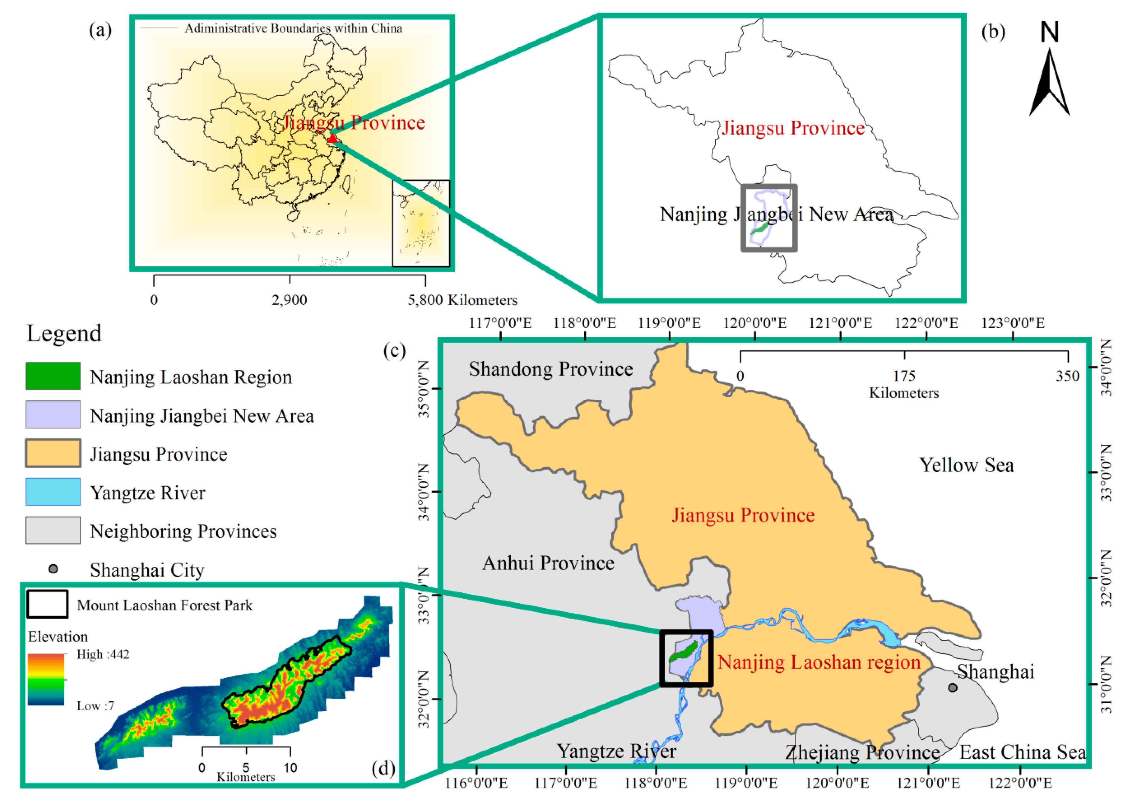
Figure 1. Overview of the study area: locations of (a) Jiangsu Province within China; (b) the Nanjing Jiangbei New Area (NJNA) within Jiangsu Province; and (c,d) the elevation map of the study area (Nanjing Laoshan Region (NLR) including Mount Laoshan Forest Park (MLFP)) near the Yangtze River within NJNA.
Remotesensing 12 00155 g001
Figure 2. Distribution of the color composite maps of satellite imagery used in this study at the resolution of 5 m for 2002, 2009, 2016, and 2016 in a false-color combination of red, green, and blue, namely, shortwave infrared, near infrared, and red for SPOT imagery in 2002, near infrared, red, and green for RapidEye and SPOT imagery in 2009 and 2016, and blue, green, and red for RapidEye imagery in 2017. The enlarged areas present more detailed views of the rectified imagery.
Remotesensing 12 00155 g002
Figure 3. Maps of land cover types from 2002 to 2023 including first four maps for 2002–2017 produced from imagery used in this study, two maps in 2016 predicted by the CA-Markov and STSM models, and two maps in 2018 and 2023 predicted by the CA-Markov model.
Remotesensing 12 00155 g003
Figure 4. Distribution of spatially consistency and inconsistency based on analysis comparing cellular automation-Markov (a,d) and a state-and-transition simulation model (b,e) based predicted land cover map and the object-oriented classification-based actual land cover map (c) in 2016.
Remotesensing 12 00155 g004
Figure 5. Area and percentage of area covered by four land cover types (cropland, forest, urban, and water) from 2002 to 2023 for the entire NLR.
Remotesensing 12 00155 g005
Figure 6. Change in forest cover between 2002 and 2023 including three 7-year intervals (2002–2009, 2009–2016, and 2016–2023) showing the spatial and temporal pattern of unchanged non-forest, unchanged forest, forest gain, and forest loss in the NLR, China. The blue line is the boundary of Nanjing MLFP.
Remotesensing 12 00155 g006
Figure 7. Change in forest gain, loss, and net change in NLR and MLFP, Jiangsu, China, from 2002 to 2023.
Remotesensing 12 00155 g007
Figure 8. Change in forest fragmentation during 2002–2023 calculated by the spatial scale defined by neighborhood size (27 × 27) in NLR, Jiangsu, China. FAD, forest area density.
Remotesensing 12 00155 g008
Figure 9. Forest fragmentation pattern measurements based on forest area density (FAD) values calculated by the spatial scale defined by neighborhood size (27 × 27) over each forest pixel in 2002 (a), 2009 (b), 2016 (c), and 2023 (d). Three enlarged areas (1, 2, and 3) present more detailed views of forest fragmentation from bottom to top in 2016.
Remotesensing 12 00155 g009
Figure 10. Forest fragmentation pattern measurements by forest area density (FAD) values from multi-source data including high resolution RapidEye data (a), PALSAR forest/non-forest (b), and China’s GlobeLand30 forest/non-forest (c) for the neighborhood size of 27 × 27 over each forest pixel in 2009.
Remotesensing 12 00155 g010
Figure 11. Fragmentation class area characterized by six forest area density proportion values in the neighborhood size of 27 × 27 and calculated from three resolution data-based forest/non-forest products including the forest/non-forest product (5 m) generated in this study (“This study”), PALSAR forest/non-forest (25 m; “PALSARfnf”) in 2009, and China’s GlobeLand30-based forest/non-forest (30 m; “GLC30”) in 2010.
Remotesensing 12 00155 g011
Figure 12. Spatial patterns of forest loss and gain related to the forest fragmentation regions from 2002 to 2023. For example, “interior gain” means “forest area gain was adding forest interior;” “interior loss” means “forest area loss was removing forest interior”. See Table 3 for definitions of forest area density classes.
Remotesensing 12 00155 g012
Table 1. Summary of high-resolution satellite data used.
DatasetDateBandResolution (Pan/Multispectral, m)
SPOT511/9/2002Pan, Green, Red, Near infrared, Shortwave infrared2.5, 10
SPOT75/12/2016Pan, Blue, Green, Red, Near infrared1.5, 6
RapidEye6/25/2009, 7/25/2017Blue, Green, Red, Red edge, Near infrarednon, 5
Table 2. The parameter settings of segmentation as well as the chosen of the numbers of regions of interest (ROIs) used for training of classification algorithm.
DatasetImage CompositeSpectral DetailSpatial DetailMinimum Segment SizeNo. of ROIs
SPOT5Band 3, 2, 120101680 points per type (20 points for water)
SPOT7Band 4, 3, 220101680 points per type (20 points for water)
RapidEyeBand 5, 4, 318101280 points per type (20 points for water)
Table 3. Summary of six fragmentation classes based on forest area density (FAD).
No.FAD ClassFAD Range [44]New FAD Range (This Study)Fragmentation Level
1RareFAD < 10%0 ≤ FAD < 20%Highly fragmented
2Patchy10% ≤ FAD < 40%20% ≤ FAD < 40%Medium fragmentation
3Transitional40% ≤ FAD < 60%40% ≤ FAD < 60%Medium fragmentation
4Dominant60% ≤ FAD < 90%60% ≤ FAD < 90%Medium fragmentation
5Interior90% ≤ FAD < 100%90% ≤ FAD < 100%Limited fragmentation
6IntactFAD = 100%FAD = 100%Not fragmented
Table 4. Summary of the forest cover products used in forest fragmentation pattern analysis.
ProductsResolutionForest DefinitionAlgorithmsAccuracy
PALSAR FNF25 m (PALSAR)Canopy cover over 10%,
and the area must be larger than 0.005 km2
Backscatter
thresholds
UA: 95.04%,
PA: 81.51%,
OA: 91.25%
GLC3030 m (Landsat)Canopy cover over 30%
(including sparse woods over 10–30%)
MLC + Expert
interpretation
UA: 83.58%
OA: 80.33%
This study5 m (RapidEye)Canopy cover over 10%Object-oriented + SVM
OA: overall accuracy; UA: Users’ Accuracy; PA: Producers’ Accuracy; MLC, Maximum Likelihood Classification; SVM, Support Vector Machine.
Table 5. The accuracy assessments of land cover maps in 2002, 2009, 2016, and 2017.
2002200920162016 CA-Markov2016 STSM2017
Overall accuracy83.75%90.85%90.30%69.40%54.95%92.25%
Kappa coefficient0.780.880.870.590.390.90
Table 6. Changes of annual deforestation rate from 2002 to 2023 during several periods.
YearForest Area for Two Dates (km2)Annual Deforestation Area (km2 yr−1)Annual Deforestation Rate (% yr−1)
2002–2009209.4, 185.33.451.57
2009–2016185.3, 157.14.032.04
2016–2017157.1, 153.14.012.6
2016–2023157.1, 123.94.752.78
2018–2023133.1, 123.91.851.35
2002–2023209.4, 123.94.071.64
Table 7. Annual percentage of each fragmentation class characterized by six forest area density proportion values (0–19%, 20–39%, 40–59%, 60–89%, 90–99%, and 100%) in the neighborhood size of 27 × 27.
Year0–19%20–39%40–59%60–89%90–99%100%≥90%
20020.10.62.315.923.757.481.1%
20090.31.34.422.523.348.271.5%
20160.72.98.025.518.144.862.9%
20170.93.37.823.917.746.464.1%
20183.16.39.121.912.147.559.6%
20231.43.78.521.012.153.365.4%
Table 8. Summary of forest area change and its rate from 2002 to 2023.
%Net ChangeForest Interior and Intact (%)Total Forest Area (%)Ratio
2002–2009−14.19−12.161.17
2009–2016−18.28−15.971.15
2016–2023−18.57−17.661.05
2002–2023−43.44−41.91.04