Abstract
Fine classification of vegetation types has always been the focus and difficulty in the application field of remote sensing. Unmanned Aerial Vehicle (UAV) sensors and platforms have become important data sources in various application fields due to their high spatial resolution and flexibility. Especially, UAV hyperspectral images can play a significant role in the fine classification of vegetation types. However, it is not clear how the ultrahigh resolution UAV hyperspectral images react in the fine classification of vegetation types in highly fragmented planting areas, and how the spatial resolution variation of UAV images will affect the classification accuracy. Based on UAV hyperspectral images obtained from a commercial hyperspectral imaging sensor (S185) onboard a UAV platform, this paper examines the impact of spatial resolution on the classification of vegetation types in highly fragmented planting areas in southern China by aggregating 0.025 m hyperspectral image to relatively coarse spatial resolutions (0.05, 0.1, 0.25, 0.5, 1, 2.5 m). The object-based image analysis (OBIA) method was used and the effects of several segmentation scale parameters and different number of features were discussed. Finally, the classification accuracies from 84.3% to 91.3% were obtained successfully for multi-scale images. The results show that with the decrease of spatial resolution, the classification accuracies show a stable and slight fluctuation and then gradually decrease since the 0.5 m spatial resolution. The best classification accuracy does not occur in the original image, but at an intermediate level of resolution. The study also proves that the appropriate feature parameters vary at different scales. With the decrease of spatial resolution, the importance of vegetation index features has increased, and that of textural features shows an opposite trend; the appropriate segmentation scale has gradually decreased, and the appropriate number of features is 30 to 40. Therefore, it is of vital importance to select appropriate feature parameters for images in different scales so as to ensure the accuracy of classification.
1. Introduction
Vegetation is the main component of the ecosystem and plays an important role in the process of material circulation and energy exchange on land surface. Various vegetation types have different responses to the ecosystem. Monitoring vegetation types is of great significance for mastering its current situation and changes and promoting the sustainable development of resources and environment [1,2]. The application of remote sensing technology in the investigation and monitoring of vegetation types is the focus and hotspot in current study. In recent years, a large number of studies on vegetation classification have been carried out by widely using remote sensing technology [3,4]. However, due to the widespread phenomenon of spectral confusion, the number of types that can be identified and the classification accuracy still need to be improved in the process of remote sensing classification for vegetation types, especially in the tropical and subtropical areas where vegetation distribution is fragmented, types are multitudinous, and planting structures are diverse [5,6]. Remote sensing images with high spatial resolution significantly enhance the structural information of vegetation, making it possible to utilize the spatial combination features of ground objects. However, due to the band number constraint, the identification ability of vegetation types is still limited [7,8]. Hyperspectral load has the ability to acquire continuous spectral information within a specific range, thus being able to capture subtle spectral characteristics of ground objects, which makes it possible to accurately identify vegetation types [9]. In recent years, the application of Unmanned Aerial Vehicle (UAV) in remote sensing has been increasingly expanded owning to UAV’s academic and commercial success [10,11]. Due to the low flying height and limited ground coverage, the resolution of images obtained by UAV-based hyperspectral cameras can reach 2–5 cm or less [12], which makes UAV hyperspectral images have both hyperspectral and high spatial characteristics and provides an important data source for the classification of vegetation types in highly fragmented planting areas [13].
There are many difficulties in the interpretation of centimeter-level UAV hyperspectral images. On one hand, with the improvement of image spatial resolution, the information of ground objects is highly detailed, the differences of spectral characteristics for similar objects become larger, and the spectra of different objects overlap with each other, promoting the intra-class variance to be larger and the inter-class variance to be smaller. The phenomena of spectral confusion occur in a large number, which weakens the statistical separability of the image spectral field and makes the identification result uncertain [14,15]. On the other hand, UAV hyperspectral images with centimeter-level resolution can provide rich spatial features, and blade shapes can even be clearly visible. Therefore, facing the problems of ultra-fine structural information and mixed spectral information in UAV hyperspectral images, balancing the spatial and spectral information to effectively identify vegetation types has to be solved. Traditional spectral interpretation methods based on image processing in medium and low resolution face great difficulties in interpreting complex features of high resolution. Object-based image analysis (OBIA) has gained popularity in recent years along with the increase of high-resolution images. It takes both spectral and spatial (texture, shape and spatial combination relation) information into account to characterize the landscape, and generally outperforms the pixel-based method for vegetation classification, particularly with high resolution images [16,17,18,19].
Scholars have been working to enhance the spatial resolution of images to improve the accuracy of clustering, detection and classification; it usually works when the size of the resolution is suitable for specific scene targets, which is related to the actual morphological and structural characteristics of these targets [20,21,22]. Actually, the spatial resolution variation of remote sensing images will lead to differences in the expression of information content, resulting in scale effect in related results. In particular, scholars argued that the appropriate spatial resolution is related to the scales of spatial variation in the property of interest [23,24,25]. Because of the complicated combinations of leaf structure and biochemistry, crown architecture and canopy structure, the spectral separability is altered by the scale at which observations are made (i.e., the spatial resolution). The spatial scale problem is the key to the complexity of type identification [26]. Due to the lack of images under synchronous multi-scale observation, the appropriate scale for vegetation type identification has not been effectively solved [27]. Scholars have generally conducted relevant study on the spatial scale effect of vegetation type identification based on multi-scale images generated after resampling [28,29,30]. For example, Meddens resampled 0.3 m digital aerial images to 1.2, 2.4 and 4.2 m based on Pixel Aggregate method and classified healthy trees and insect attacking trees using Maximum Likelihood classifier. The result shows that the identification accuracy of 2.4 m images is the highest [31]. Roth spatially aggregated the fine resolution (3–18 m) of airborne AVIRIS to the coarser resolution (20–60 m) for accurate mapping of plant species. The result shows that the best classification accuracy is at the coarser resolution, not the original image [32]. Despite these achievements, most research has been based on images at meter-level and sub-meter-level resolutions. However, for more fragmented planting structures and based on finer spatial resolution (e.g., centimeter level), how to balance the relationship between monitoring target scale and image scale and on which resolution the vegetation types can be accurately identified have to be solved. Especially in view of the limited ground coverage of UAV images, it is of great significance to flight at a proper spatial scale to maximize the coverage while ensuring classification accuracy.
This study is mainly aimed at: (1) Making full use of the hyperspectral and high spatial characteristics of UAV hyperspectral images to realize the fine classification of vegetation types in highly fragmented planting areas and (2) obtaining the scale variation characteristics of vegetation type identification for UAV images, exploring the appropriate scale range to provide reference for UAV flight experiment design, remote sensing image selection and UAV image application of vegetation classification in similar areas.
2. Study Area and Data Sources
2.1. Overview of the Study Area
The study area is located in Xingbin District, Laibin City, Guangxi, China, East Asia (Figure 1). Laibin City is located between 108°24′–110°28′E and 23°16′–24°29′N, with mountains and hills accounting for 65%, and other areas are platforms and plains. It boasts a subtropical monsoon climate with warm weather, abundant rain and insignificant seasonal changes. Laibin City is rich in vegetation resources, which has the typical characteristics of complex planting structure, abnormal fragmented field parcels, terrain cutting in southern China. Different vegetation types show irregular and staggered distribution, which brings great difficulties to the fine classification of vegetation types. The main vegetation types in Laibin City are sugarcane, eucalyptus, citrus, etc. Laibin City is one of the key sugarcane production bases in China, taking the sugarcane production as the pillar industry. It has obvious advantages in planting fast-growing forests, and high-quality eucalyptus trees are widely planted. In addition, there are many kinds of horticultural crops in Laibin City, of which citrus is the most widely cultivated and distributed.
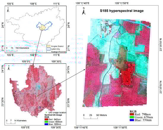
Figure 1.
Geographic location and UAV image of the study area.
2.2. Field Investigation and UAV Image Acquisition
Xingbin District is the only municipal district in Laibin City. A field survey was carried out in the south-central part of Xingbin District from December 7 to 10, 2017 (Figure 1). At that time, sugarcane entered the mature period and began to harvest gradually; most of the late rice has been harvested. From 10:00 to 13:00 on December 10, two consecutive hyperspectral images of UAV were acquired, covering an area of 230 × 330 m. A commercial snapshot hyperspectral imaging sensor (S185) onboard a multi-rotor UAV platform was used in this study. The S185 sensor employs two charge-coupled device (CCD) detectors with the 6.45 μm pixel size and the focal length of 23 mm. The S185 multi-rotor UAV system mainly includes: Cubert S185 hyperspectral data acquisition system, six-rotor electric UAV system, three-axis stabilized platform and data processing system. The S185 was radiometrically corrected with reference measurements on a white board and dark measurements by covering the black plastic lens cap prior to the flight. The reflectance was obtained by subtracting the dark measurement from the actual measured values during the flight and the reference values and then divided by this reference [33]. The measurement time to capture a full hyperspectral data cube is consistent with the automatic exposure time for white board reference measurement, about 1ms in a clear sky. With the flight height of 100 m, flight speed of 4.8 m/s, sampling interval of 0.8 s, heading overlap rate of about 80% and lateral overlap rate of about 70%, hyperspectral cubes of 125 effective bands (450–946 nm) and panchromatic images with the spatial resolution of 0.025 m were acquired synchronously. Totally 898 hyperspectral cubes with 12-bit radiometric resolution and with the size of 50 × 50 pixels were created. Accordingly, there were 898 panchromatic images with the size of 1000 × 1000 pixels. The typical vegetation types in the UAV coverage image are sugarcane, eucalyptus and citrus. In addition, there are also some vegetables, weeds and other vegetation types. All vegetation types are distributed alternately and extremely fragmented. A handheld Global Navigation Satellite System (GNSS) receiver (Juno SB, Trimble Navigation Limited, Sunnyvale, CA, USA) was used to record the position and category information of sample points, with a positioning accuracy of about 3 m. A total of 63 samples were recorded, which were evenly distributed throughout the study area.
2.3. Preprocessing of UAV Hyperspectral Image
The preprocessing of S185 hyperspectral image mainly includes image fusion and mosaic [34]. Each hyperspectral cube and the corresponding panchromatic image synchronously collected were fused by using Cubert-Pilot software (Cubert GmbH, Ulm, Baden-Württemberg, Germany), and the fused hyperspectral cubes were obtained with a spatial resolution of 0.025 m [35]. The automatic image mosaic software Agisoft PhotoScan (Agisoft, St. Petersburg, Russia) was used for its stated accuracy 1–3 pixels and the high-quality mosaic [36]. By capturing overlapping images with a certain overlap rate, all the hyperspectral cubes were stitched together based on the point clouds of the panchromatic images [34]. Since the Position and Orientation System (POS) was not equipped onboard the UAV, the UAV hyperspectral image was geometrically corrected with reference to the 0.14 m Google Earth (GE) image dated 7 December 2016. As the spectrum less than 0.85 μm was consistent with that of vegetation, hyperspectral data in the range of 0.45–0.85 μm were used in the study, totaling 101 bands [37,38]. The corresponding wavelengths of 101 bands are available in Appendix A.
In order to explore the influence of spatial scale on vegetation classification of UAV images, the 0.025 m image was resampled to 0.05, 0.1, 0.25, 0.5, 1, 2.5 m, a total of 7 pixel scales according to the spatial resolution range of most UAV images. As the smoothing or sharpening effects of the Nearest Neighbor, Bilinear and Cubic Convolution would affect the result analysis [39,40,41], the Pixel Aggregate was used to reduce the resolution of images. The Pixel Aggregate averages the resolution units into a larger one, avoiding the debate on the exact definition of spatial resolution and how to measure it [42], which has been widely used in multi-scale analysis [25,43,44,45,46].
2.4. Reference Data
Based on the field observations and the recorded 63 field samples, a total of 59 polygons were manually outlined as training samples. The number of training polygons and corresponding pixels in multi-scale UAV images are shown in Table 1. In addition, a hand-drawn ground-truth reference image was delineated in detail for validation. Figure 2 illustrates the distribution of the reference image.

Table 1.
A list of training polygons and corresponding pixels in multi-scale images.
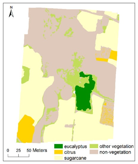
Figure 2.
Ground truth reference image.
3. Methods
Based on UAV hyperspectral images of 7 different scales, sugarcane, eucalyptus, citrus and other vegetation were classified by using object-based image analysis (OBIA). Specifically, it included: (1) selecting appropriate scale for multi-resolution segmentation; (2) using the mean decrease accuracy (MDA) method for feature evaluation and selection; (3) selecting the classifiers of Support Vector Machines (SVM) and Random Forest (RF) to classify vegetation types of multi-scale images and comparing their accuracy differences; (4) analyzing the variation of appropriate segmentation parameters and feature space of multi-scale images, and discussing the influence of spatial scale variation on vegetation classification of UAV images.
3.1. Multi-Resolution Segmentation
Image segmentation is the first step of OBIA. It is a process of dividing an image into several discrete image objects (IOs) with unique properties according to certain criteria [47]. The accuracy of image segmentation significantly affects the accuracy of OBIA [48]. A bottom up region-merging technique based on the fractal net evolution algorithm proposed by Baatz and Schäpe was used for multi-resolution segmentation [49]. As the most widely used method, it can generate highly homogeneous segmentation regions, thus separating and representing ground objects in the best scale [50]. In the study, two segmentations were performed, creating two levels of IOs. A series of interactive "trial and error" tests were used to determine the proper segmentation parameters [51,52]. Six spectral bands including blue, green, red, red edge I, red edge II and near-infrared were used as inputs. A small-scale factor was used for the first segmentation to maximize the separation of vegetation and non-vegetation. In the second segmentation, three scale factors were set separately to prevent the objects being too fragmented and the appropriate segmentation of the three was determined by the classification accuracy.
3.2. Feature Extraction
In the process of OBIA, the features related to the IOs can be extracted from the UAV image. The ideal features should reflect the differences between the target types.
Sugarcane, citrus and eucalyptus are broadleaf vegetation, showing different spatial distribution features in high spatial resolution images. Sugarcane stalks are 3–5 m high, with clumps of leaves. The leaves are about 1m long and 4–6 cm wide, the edges of which are serrated and rough. The rows are 80–100 cm apart, showing the characteristics of fine and compact distribution. Citrus is an evergreen small tree with a height of about 2 m and a round crown of less than 2 m. The plant spacing is 1.5–2 m. The leaves are ovate-lanceolate, with a large size variation and a length of 4–8 cm. It shows a feature of regular, sparse and circular crown distribution. Eucalyptus is an evergreen dense-shade tall tree with a height of 20 m. Its crown is triangular spire-shaped, with small crown and opposite leaves in heart or broadly lanceolate shape, showing a feature of dense distribution.
In this study, as shown in Table 2, 149 features associated with the IOs derived from the second segmentation in 4 categories including spectrum, vegetation index, texture and shape have been extracted. (1) Commonly used parameters such as reflectance, hue, intensity, brightness, maximum difference (Max.diff), standard deviation (StdDev) and ratio were used to analyze the spectral features of vegetation. (2) 18 vegetation indices were selected (Table 3), including not only the broadband index that could be calculated based on traditional multi-spectral images but also the red edge index that was more sensitive to vegetation types. (3) Two shape features, shape index and compactness, were used to represent the shape of vegetation. (4) The widely used gray-level co-occurrence matrix (GLCM) [53] and gray-level difference vector (GLDV) [54] were used to extract textural features.
Table 2.
Spectral, vegetation index, textural and shape features used.
Table 3.
Vegetation index and calculation method.
3.3. Feature Evaluation and Reduction
High-dimensional data usually need feature selection before machine learning. The significance of feature selection lies in reducing data redundancy, strengthening the understanding of features, enhancing the generalization ability of models and improving the processing efficiency. Random Forest (RF) can effectively reduce the data dimension while ensuring the classification accuracy, which is a machine learning algorithm composed of multiple classification and regression trees (CART) proposed by Breiman [71]. It is widely used in classification and identification of images and selection of high-dimensional features [72,73]. The mean decrease accuracy (MDA) method of RF was adopted for feature importance evaluation, which could disturb the eigenvalue order of each feature and then evaluate the importance of the feature by measuring the influence of this change on the accuracy of the model. If a feature is important, its order change will significantly reduce the accuracy.
On the basis of MDA results, all the features are ranked from big to small according to the feature importance, and different number of features will be used successively to classify vegetation types. In order to eliminate feature redundancy that might be caused by repeated participation of adjacent 101 reflectance bands, the following feature reduction principle is adopted based on feature importance evaluation:
For 101 bands, they are first ranked in order of feature importance from big to small. When a band is retained, the two adjacent bands above and below will be deleted.
Sometimes, it may occur that the interval between the band to be retained and the band already retained is 3, which is also acceptable. However, if the interval is 4, this band should be deleted, and its upper or lower band should be retained to ensure that the retained band has relatively strong importance and the number of bands deleted between the retained bands is 2 or 3.
For example, if the first important band is the 64th band, it should be retained first, and the 62nd, 63rd, 65th and 66th bands should be deleted at the same time. If the second important band is the 61st or 60th band, both cases are acceptable because it can ensure that the number of deleted bands is 2 or 3. However, if the second important band is the 59th band, it needs to be deleted, and the more important one of the 58th or 60th band needs to be retained according to the importance of the two.
3.4. Classifier
Two supervised classifiers were considered in this paper: Support Vector Machines (SVM) and Random Forest (RF).
SVM is a non-parametric classifier [74]. Adopting the principle of structural risk minimization, it automatically selects important data points to support decision-making. It provides a brand-new solution for classification of ground objects in high-resolution images with extraordinary efficiency. In this study, we used Radial Basis Function Kernel (RBF) function because of its outperformance in classification [75]. Two important classifier parameters need to be determined, including RBF kernel parameter gamma and penalty factor c. A moderate error penalty value (c = 100) and a gamma equaling to the inverse of the feature dimension were configured to facilitate the comparison between the different classification results related to different feature numbers [76,77].
As mentioned above, RF is a non-parametric ensemble learning algorithm [71], which is composed of multiple decision-making trees. In the process of building decision-making trees, the splitting of each point is determined by Gini coefficient criterion to realize the best variable splitting. RF has the characteristics of fast learning speed, strong robustness and generalization ability. It has the abilities to analyze and select complex interaction features, being widely used in computer vision, human identification, image processing and other fields. Two important parameters need to be determined, including ntree (the number of decision trees executing classification) and mtry (the number of input variables used at each node) [78]. Different numbers of ntree were tested from 50 to 150 at 10 tree intervals. Classification accuracy did not change much as the number changed. Consistently used ntree (ntree = 50) and mtry equaling to the square root of the feature dimension were configured to facilitate the comparison between the different classification results related to different feature numbers.
4. Results
4.1. Results of Multi-Resolution Segmentation and Vegetation Information Extraction
Two segmentations were performed by multi-resolution segmentation. As the most important segmentation parameter, segmentation scale greatly affects the identification results of vegetation types. In order to distinguish vegetation information from non-vegetation to the greatest extent, the scale of the first segmentation should be as small as possible so that the segmentation object would not contain both vegetation and non-vegetation information (Table 4). For multi-scale images, six bands including blue (band1), green (band26), red (band56), red edge I (band65), red edge II (band74) and near-infrared (band88) were used as inputs, and the weight of each band was 1. By the “trial and error” method and previous study experience [79,80], the first segmentation was completed under the spectral parameter of 0.9, shape parameter of 0.1, compactness of 0.5 and smoothness of 0.5.
Table 4.
Scale parameters for first segmentation of multi-scale images.
NDVI and mNDVI705 were jointly applied to extract vegetation information. NDVI can reflect the distribution density and grow conditions of vegetation to the maximum extent, so it is often regarded as the most important vegetation index for vegetation information extraction. However, when NDVI was used alone to extract vegetation information, a few marginal areas of vegetation, ridges of field and harvested rice stubbles were confused with vegetation information, so mNDVI705 was added to help the extraction of vegetation information. Derived from NDVI705, mNDVI705 takes the specular reflection characteristics of leaves into consideration and is good at capturing the subtle characteristics of leaf senescence and small changes in leaf canopy. Thus, it has been widely used in fine agriculture, forest monitoring and vegetation stress monitoring [81,82,83]. The multi-parameter threshold method was adopted, i.e., NDVI and mNDVI705 respectively take thresholds. When NDVI was greater than or equal to 0.29 and mNDVI705 was greater than or equal to 0.256, vegetation information in the study area would be accurately extracted.
On the basis of vegetation information that had been extracted, the objects of vegetation information were segmented for the second time, in order to utilize the textural features of objects and ensure that the classification results are not excessively fragmented. And then, citrus, sugarcane, eucalyptus and other vegetation were identified on this basis. Three different segmentation scales were respectively set for multi-scale images, and then the appropriate segmentation scale for multi-scale images was determined by the classification accuracy (Table 5).
Table 5.
Appropriate scale parameters for secondary segmentation of multi-scale images.
Taking the secondary segmentation result of 0.25 m image in Figure 3d,e,f at three scales as an example, when the parameter of segmentation scale is too small, the objects cannot reflect rich textural information. If it is appropriate, the textural structure can be effectively reflected without being too fragmented. Once it is too big, for vegetation types with similar spatial and spectral features, the probability of objects containing different vegetation types will increase.
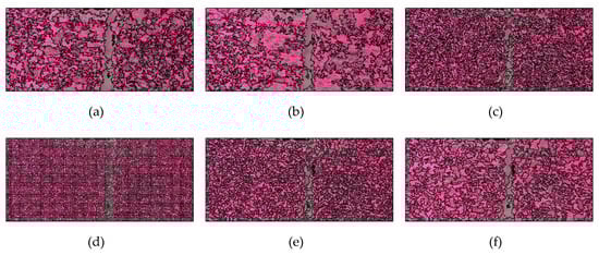
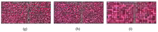
Figure 3.
Local representation of secondary segmentation for multi-scale images: (a) 0.025 m (segmentation scale: 2500); (b) 0.05 m (segmentation scale: 1000); (c) 0.1 m (segmentation scale: 100); (d) 0.25 m (segmentation scale: 25); (e) 0.25 m (segmentation scale: 50); (f) 0.25 m (segmentation scale: 100); (g) 0.5 m (segmentation scale: 50); (h) 1 m (segmentation scale: 25); (i) 2.5 m (segmentation scale: 25).
With the decrease of spatial resolution, the occurrence probability of mixed pixels increases. In order to ensure the homogeneity of vegetation types in the same object, the segmentation scale gradually decreases. However, the appropriate segmentation scale does not show a simple recursive variation with spatial resolution or data volume. For images with 0.1–2.5 m spatial resolution, the segmentation scale is concentrated in 25–100, while the segmentation scales for 0.05 and 0.025 m images rapidly rise to 1000 and 2500, which shows that the ability of the classifier to correctly recognize larger objects is enhanced in images with centimeter-level resolution.
4.2. Results of Feature Analysis
4.2.1. Importance Variation of Different Feature Types
To evaluate the feature importance variation of multi-scale images and rank the features involved in the classification, the importance of 149 features was measured by MDA method. In the process of MDA, based on the 149 features calculated for the training IOs derived from the training rectangles, the importance scores of 7 multi-scale images in each second segmentation scale were obtained, respectively. The feature importance was separately analyzed in the categories of spectrum, vegetation index, texture and shape for multi-scale images under the condition of the appropriate segmentation scale.
1. Importance Analysis of Spectral Features in Multi-Scale Images
According to the normalized measurement results of importance for 101 reflectance features in multi-scale images and their boxplot distribution, as shown in Figure 4a, for 0.025–0.5 m images, the important spectral ranges are located in red edge I, followed by red, green and blue regions. With the decrease of spatial resolution, the importance of red edge I for 1–2.5 m images decreases, and the green and yellow bands increase in importance.
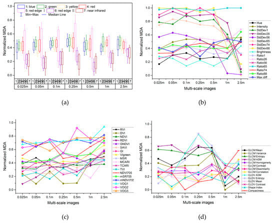
Figure 4.
Importance measurement results of spectral, vegetation index, textural and shape features in multi-scale images. (a) Boxplot of the normalized mean decrease accuracy (MDA) for 101 reflectance features; (b) normalized MDA for other spectral features; (c) normalized MDA for vegetation index features; (d) normalized MDA for textural and shape features.
According to the normalized measurement results of importance for other spectral features in multi-scale images, as shown in Figure 4b, Ratio65 is in the forefront of importance evaluation in all scale images, i.e., the contribution ratio of red edge I is in the important position. For 0.025–0.5 m images, the features of StdDev are of great importance, but their importance declines rapidly with the decrease of spatial resolution. The importance of intensity, hue and brightness of 2.5 m image increases.
2. Importance Analysis of Vegetation Index Features in Multi-Scale Images
As shown in Figure 4c, with the decrease of spatial resolution, the importance of vegetation index features increases. The vegetation indices in the forefront of importance evaluation are all related to the red edge. Among broadband indices that can be calculated based on traditional 4-band multi-spectral images, VIgreen is of greater importance in all scale images; and NDVI, the most widely used index, is of greater importance in 0.1 m image.
3. Importance Analysis of Shape and Textural Features in Multi-Scale Images
As shown in Figure 4d, with the decrease of spatial resolution, the importance of textural features increases slightly in fluctuation and then decreases. For 0.025–0.5 m images, GLCM ASM, GLCM Entropy and GLCM Mean are stable and in the forefront of importance evaluation. For 0.1–0.5 m images, GLDV ASM and GLDV Entropy are more important. In general, the importance of textural features for 1 and 2.5 m images is weakened, which is reflected in the reduction of pixel numbers contained in low-resolution images for the object scale, resulting in textural difference weakening of different vegetation types in low-resolution images. Shape features are not of sufficient importance in multi-scale images, and only the 2.5 m image is of strong importance for the compactness feature.
4.2.2. Variation of Feature Types within Different Feature Groups
In order to eliminate feature redundancy that might be caused by repeated participation in classification of adjacent 101 reflectance bands, the feature reduction principle in Section 3.3 was adopted. Due to the different feature importance order of 101 bands for the 7 scale images, accordingly, the number of deleted bands among the retained bands was 2 or 3, which was not exactly the same, resulting in a slight difference in the number of retained bands. After the feature reduction of 101 bands, the number of retained bands was 29–31 for multi-scale images. Together with other spectral, vegetation index, textural and shape features, the total number of features after reduction was 77–79. In the following analysis, the value of "80 features" was used instead of "77–79" for uniform marking.
Finally, according to the importance from big to small, the final features were divided into 8 groups with 10 features in each group. The number of features for different feature types in each group was divided by the total number of this feature type. The results show that the proportion of different feature types in each group is different (Figure 5). In general, spectral features are distributed in all groups with little difference. The proportion of vegetation index features for multi-scale images in each group is quite different, which shows that the importance of vegetation index features increases as the spatial resolution decreases. Textural features are mainly distributed in the last 4 groups. In the first 4 groups, textural features are mainly distributed in images with high spatial resolution, while the textures in low-resolution images are not of sufficient importance. Shape features perform poorly in each scale image and are mainly distributed in the latter 3 groups. Compared to images with high spatial resolution, shape features in low-resolution images are enhanced. These results are consistent with previous studies [8,54,78,84]. In these studies, the spectral and vegetation index features make more significant contributions to the species classification of high spatial resolution images than the textural and shape features. Specifically, only a small percentage of texture or shape features are selected for classification. The majorities and most important features are spectral and vegetation index features.
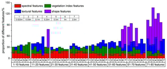
Figure 5.
Distribution of feature types within feature groups in multi-scale images.
4.3. Classification Results
According to the results of feature importance evaluation and selection, SVM classifier was used to classify multi-scale images by using different segmentation scales and different number of features successively, adding 10 features each time. This means that the first 10 features will be used for the first classification and 80 features will be used for the eighth classification. The overall accuracy (OA) and Kappa coefficient were used to evaluate the classification accuracy based on the ground-truth reference image covering the whole study area [85]. Figure 6 presents the classification results of multi-scale images based on SVM classifier under the condition of appropriate segmentation scale and feature number.
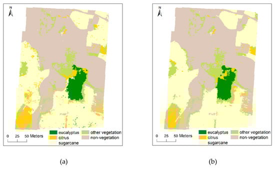
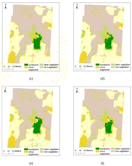
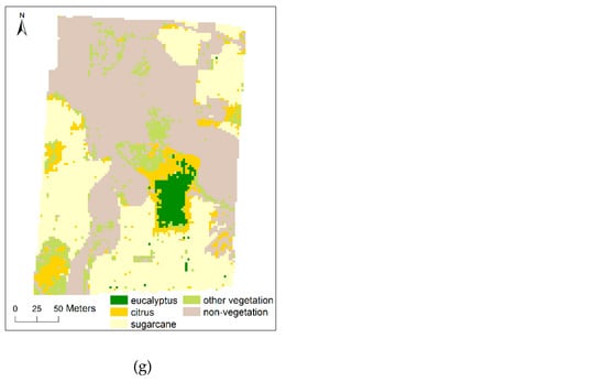
Figure 6.
Classification results of the study area for multi-scale UAV images based on SVM classifier. The UAV image and the ground truth reference image of the study area are available in Figure 1 and Figure 2, respectively; (a) 0.025 m (segmentation scale: 2500, feature number: 40); (b) 0.05 m (segmentation scale: 1000, feature number: 30); (c) 0.1 m (segmentation scale: 100, feature number: 40); (d) 0.25 m (segmentation scale: 50, feature number: 30); (e) 0.5 m (segmentation scale: 50, feature number: 30); (f) 1 m (segmentation scale: 25, feature number: 30); (g) 2.5 m (segmentation scale: 25, feature number: 40).
RF classifier was used to perform classification to verify the results of SVM classifier. As shown in Table 6, compared with the classification results of vegetation type for multi-scale images based on SVM classifier under appropriate segmentation scale and feature number, the results of RF classifier under corresponding conditions were slightly lower than those of SVM, and the OA decreased by 1.3%–4.2%, which was consistent with previous study results [86,87,88]. In these studies, SVM classifier has higher classification accuracy and stronger robustness than RF. Furthermore, classification experiments based on all 149 features were carried out by SVM and RF classifiers. Compared to the results using all 149 features, it shows that the classification accuracy of SVM classifier using the appropriate number of features has been greatly improved, with the OA increasing by 2.5%–8.3%. These results are consistent with previous studies; that is, for too many spectral bands or target features, the classification performance and efficiency can be improved by eliminating redundant information [89,90]. It is worth noting that RF is insensitive to the number of features and could provide better results than SVM when using all 149 features [90].
Table 6.
Classification results of vegetation types for multi-scale images.
In addition, the pixel-based classification was performed based on 101 reflectance bands using SVM classifier (Table 6). However, due to the large data volumes of 0.025 m image with the size of 10,127 × 13,346 pixels, totally 25.4 GB, the classification becomes infeasible because of the prohibitively high time and space complexities based on the normal computer. Anyhow, from the results of other 6 scale images, OBIA outperforms pixel-based method to some extent.
5. Analysis and Discussion
5.1. Overall Accuracy Variation of Multi-Scale Images
Figure 7 shows the OA variation for multi-scale images using SVM classifier in the condition of different segmentation scales and feature numbers. It can be seen that segmentation scales and feature numbers have great influence on the classification accuracy of multi-scale images, further confirming the importance of segmentation scale optimization and multi-feature analysis.
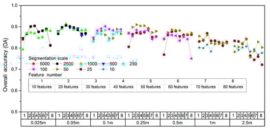
Figure 7.
Overall accuracy (OA) of multi-scale images with different segmentation scales and feature numbers.
As shown in Figure 8, the number of appropriate features for multi-scale images is 30–40. With the increase of feature number, the identification accuracy shows a trend of increasing first and then decreasing for multi-scale images, which reveals that too few features cannot achieve the purpose of high-precision identification of vegetation types, while too many features have strong correlation and information redundancy, resulting in interference information for vegetation classification.
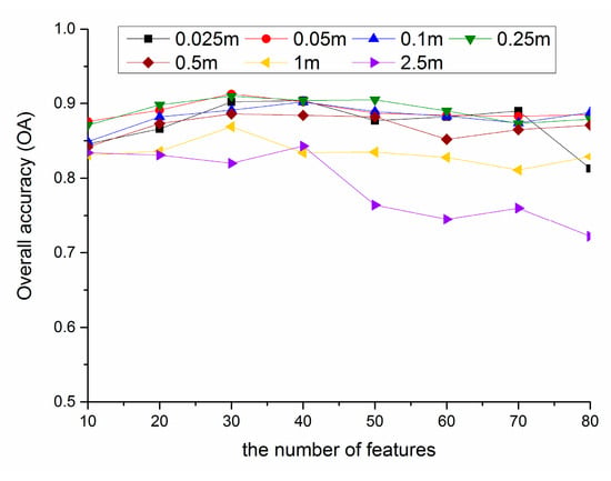
Figure 8.
Variation of overall accuracy (OA) with the number of features for multi-scale images.
Figure 9 shows the OA variation under the condition of appropriate feature number and segmentation scale with different spatial scale by using SVM classifier. As the spatial resolution decreases, the OA shows a stable and slight fluctuation, and then gradually decreases. Among them, the accuracies of 0.025, 0.05, 0.1 and 0.25 m images showed little difference and reached more than 90%. The accuracy of 0.05 m image was the highest, reaching 91.3%, followed by 0.25 m image with an accuracy of 91.0%. Since the spatial resolution of 0.5 m, the OA gradually declined from 88.6% to 84.3% with the decrease of spatial resolution. The classification accuracy of images at various scales is consistent with previous studies. For example, Underwood used 4 m AVIRIS hyperspectral image, and the classification accuracy for six communities of three invasive species reaches 75% [28]. In Cao’s study, the classification accuracy for mangrove species based on 0.15, 0.3 and 0.5 m UAV hyperspectral images reach 88.66%, 86.57% and 82.69%, respectively [91].
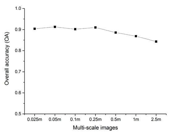
Figure 9.
Variation of overall accuracy (OA) under the condition of appropriate feature number and segmentation scale with different spatial scale.
In this case study, the OA drops if the resolution is coarser than 0.25 m. With the decrease of spatial resolution, the number of mixed pixels increase continuously, and the edge of the parcels is more likely to increase commission and omission errors. This means that the spatial resolution should reach a certain threshold to achieve decent accuracy. However, same as previous cognition, the finer the spatial resolution is not the better [31,92]. For example, the accuracy of 0.025 m image is slightly lower than that of 0.05 m and 0.25 m. This makes sense, as vegetation has specific physical size, and spatial resolution significantly finer than the certain threshold may not help the classification performance. The image with centimeter-level resolution helps us not only to understand the detailed information of vegetation types but also significantly strengthens the phenomenon of same objects with different spectrum, bringing more interference to vegetation type identification. At the same time, the ultrahigh resolution has resulted in multiple increases in information, significantly reduces the efficiency of image processing. It means that there is no need to excessively pursue finer resolution than the threshold. A low-cost imager may be sufficient. Alternatively, the UAV can fly at higher altitude with larger coverage by sacrificing the spatial resolution, which is still sufficient for vegetation classification.
5.2. Identification Accuracy Variation of Each Vegetation Type
Producer’s accuracy (PA), user’s accuracy (UA) and F-Score were used to evaluate the classification accuracy of each vegetation type, and the maximum F-score of the results based on different feature numbers was taken as the best identification accuracy of each vegetation type at various scales.
As shown in Figure 10 and Figure 11, the maximum F-score of sugarcane is the highest, reaching 92.4%–95.5% for multi-scale images. The 0.025–1 m images are not sensitive to the variation of feature numbers. The PA of sugarcane varies greatly with different feature numbers of the 2.5 m image, i.e., with the decrease of spatial resolution, the importance of feature selection increases. The maximum F-score of eucalyptus is between 82.0% and 90.4% in various scales. Except for the 2.5 m image, the variation of feature number has great influence on the identification of eucalyptus. The maximum F-score of citrus in each scale image is poorly. When 40 features of 0.25 m image participate in classification, the F-score reached the maximum, 63.39%. Then with the decrease of spatial resolution, the identification accuracy decreases greatly. The PA of citrus is relatively acceptable, while the UA performs terribly, which shows that as much citrus information as possible is extracted, while more non-citrus is identified as citrus. In addition, the variation of feature numbers has great influence on the accurate identification of citrus. Similar to citrus, the type of other vegetation receives low accuracy. When 30 features of 0.025 m image participated in classification, the F-score reached the maximum, 66.69%. Since the 0.25 m image, the identification accuracy gradually declines with the decrease of spatial resolution.
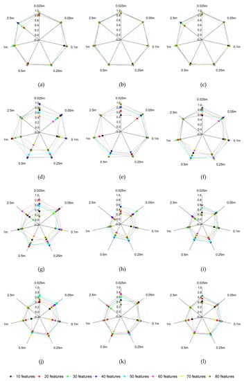
Figure 10.
Identification accuracy variation of various vegetation types with image scales and feature numbers; (a) producer’s accuracy (PA) of sugarcane; (b) user’s accuracy (UA) of sugarcane; (c) F-Score of sugarcane; (d) PA of eucalyptus; (e) UA of eucalyptus; (f) F-Score of eucalyptus; (g) PA of citrus; (h) UA of citrus; (i) F-Score of citrus; (j) PA of other vegetation; (k) UA of other vegetation; (l) F-Score of other vegetation.
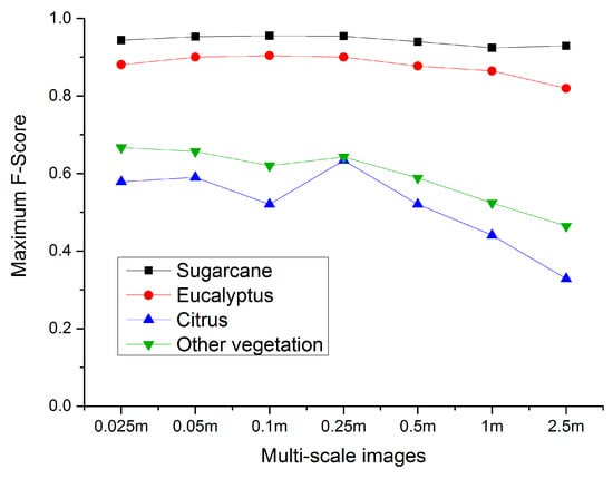
Figure 11.
Maximum F-Score variation of various vegetation types in multi-scale images.
In general, although the parcels of sugarcane and eucalyptus are irregular in shape in multi-scale images, most parcels have an area of more than 125 m2, accounting for about 20 pixels in 2.5 m image. Moreover, they are significantly different from citrus and other vegetation and are easier to be identified with accurate and stable accuracy for all 7 scales. However, citrus and other vegetation acquired unsatisfactory results, and the identification accuracies decreased greatly since the resolution of 0.25 m. Citrus plants are small, and the planting structure is sparse. The crown boundary can be segmented in images with spatial resolution better than 1m. With the decrease of spatial resolution, dwarf citrus plants and surrounding ground objects will be formed into mixed pixels. It is difficult to segment the crown boundary based on 2.5 m image. In addition, other vegetation scattered in the study area tend to be confused with citrus, resulting in the reduction of the identification accuracies for citrus and other vegetation. At the same time, the edge of each vegetation type is mostly mixed or scattered with the type of other vegetation, and the commission and omission in the classification results also occur at the edge of different vegetation types, which shows that the occurrence of mixed pixels in the transition region of different vegetation types increases with the decrease of spatial resolution, bringing greater uncertainty to the classification results of vegetation types.
6. Conclusions
This study aims to evaluate the impact of spatial resolution on the classification of vegetation types in highly fragmented planting areas based on UAV hyperspectral images. By aggregating the 0.025 m UAV hyperspectral image into coarse spatial resolutions (0.05, 0.1, 0.25, 0.5, 1, 2.5 m), we have simulated centimeter-to-meter level resolution images that can be obtained by the UAV system, and evaluated the accuracy variation of the fine classification of several vegetation types such as sugarcane, citrus and eucalyptus in southern China based on multi-scale images. The results show that the classification accuracy of vegetation types is closely related to the scale of remote sensing images. For this study area, with the decrease of spatial resolution, the OA shows a stable and slight fluctuation and then gradually decreases. The best classification accuracy does not occur in the original image but at an intermediate level of resolution. These results are consistent with similar studies on image scale, i.e., the best resolution occurs when the spectral intra-class variance is the smallest, and the class has not yet begun to mix spatially. Therefore, the ideal spatial resolution should vary according to the diversity and distribution of species in the ecosystem. Parcel size and distribution are the key factors that determine the accuracy at a given resolution. Due to the existence of small and fragmented parcels, images with coarse resolution no longer contain some original categories, such as citrus in this study, resulting in the reduction of classification accuracy of 1 and 2.5 m images. Therefore, it is important to select images of appropriate spatial scale according to the special distribution and parcel size of the study area so as to obtain more ideal classification accuracy in UAV flight experiment, data processing and application. In the process of OBIA, based on the results of multi-feature evaluation and analysis, it is successful to classify vegetation types of images in different scales by using different feature numbers and segmentation parameters. We find that with the decrease of the spatial resolution, the importance of vegetation index features increases and that of textural features shows an opposite trend; the appropriate segmentation scale decreases gradually, and the appropriate number of features is 30–40, which means that the feature parameters vary for multi-scale images. Therefore, appropriate feature parameters need to be selected for images in different scales to ensure the accuracy of classification.
There are several clear directions for future study. First, a more realistic simulation and amplification for images of fine spatial resolutions will help to improve the evaluation of potential applications of similar data in coarse resolution. The study on up-scaling of remote sensing images also shows that the spectral information of the resampled images has a strong dependence on the original images, resulting in differences with the actual observation results at a given scale [93]. The results of this study should be compared with the classification results using actual observation images for further understanding the potential impact of resolution on the classification of vegetation types. In addition, the improvement of spatial resolution will lead to greater intra-class difference and inter-class similarity, which will usually result in classification errors [94,95]. In view of the challenges and potential of ultrahigh resolution UAV images in the classification of vegetation types, advanced data analysis technologies developed in computer vision and machine learning, such as deep learning [96], should be comprehensively analyzed to improve the application capability of UAV images.
Author Contributions
Conceptualization, J.Y., T.Y. and X.G.; methodology, M.L.; investigation and data acquisition, M.L. and Z.S.; data analysis and original draft preparation, M.L., Z.Z. and X.M.; validation and writing—review and editing, Z.S., W.C. and J.L.; All authors contributed to the discussion, provided suggestions to improve the manuscript and checked the writing. All authors have read and agreed to the published version of the manuscript.
Funding
This study was funded by the Guangxi Science and Technology Development Project of Major Projects (Guike AA18118048-2) and the National Civil Space Infrastructure Project (17QFGW02KJ).
Conflicts of Interest
The authors declare no conflict of interest.
Appendix A
Table A1.
The corresponding wavelengths of 101 bands.
Table A1.
The corresponding wavelengths of 101 bands.
| Band Number | Wavelength(μm) | Band Number | Wavelength(μm) | Band Number | Wavelength(μm) | Band Number | Wavelength(μm) |
|---|---|---|---|---|---|---|---|
| 1 | 0.450 | 27 | 0.554 | 52 | 0.654 | 77 | 0.754 |
| 2 | 0.454 | 28 | 0.558 | 53 | 0.658 | 78 | 0.758 |
| 3 | 0.458 | 29 | 0.562 | 54 | 0.662 | 79 | 0.762 |
| 4 | 0.462 | 30 | 0.566 | 55 | 0.666 | 80 | 0.766 |
| 5 | 0.466 | 31 | 0.570 | 56 | 0.670 | 81 | 0.770 |
| 6 | 0.470 | 32 | 0.574 | 57 | 0.674 | 82 | 0.774 |
| 7 | 0.474 | 33 | 0.578 | 58 | 0.678 | 83 | 0.778 |
| 8 | 0.478 | 34 | 0.582 | 59 | 0.682 | 84 | 0.782 |
| 9 | 0.482 | 35 | 0.586 | 60 | 0.686 | 85 | 0.786 |
| 10 | 0.486 | 36 | 0.590 | 61 | 0.690 | 86 | 0.790 |
| 11 | 0.490 | 37 | 0.594 | 62 | 0.694 | 87 | 0.794 |
| 12 | 0.494 | 38 | 0.598 | 63 | 0.698 | 88 | 0.798 |
| 13 | 0.498 | 39 | 0.602 | 64 | 0.702 | 89 | 0.802 |
| 14 | 0.502 | 40 | 0.606 | 65 | 0.706 | 90 | 0.806 |
| 15 | 0.506 | 41 | 0.610 | 66 | 0.710 | 91 | 0.810 |
| 16 | 0.510 | 42 | 0.614 | 67 | 0.714 | 92 | 0.814 |
| 17 | 0.514 | 43 | 0.618 | 68 | 0.718 | 93 | 0.818 |
| 18 | 0.518 | 44 | 0.622 | 69 | 0.722 | 94 | 0.822 |
| 19 | 0.522 | 45 | 0.626 | 70 | 0.726 | 95 | 0.826 |
| 20 | 0.526 | 46 | 0.630 | 71 | 0.730 | 96 | 0.830 |
| 21 | 0.530 | 47 | 0.634 | 72 | 0.734 | 97 | 0.834 |
| 22 | 0.534 | 48 | 0.638 | 73 | 0.738 | 98 | 0.838 |
| 23 | 0.538 | 49 | 0.642 | 74 | 0.742 | 99 | 0.842 |
| 24 | 0.542 | 50 | 0.646 | 75 | 0.746 | 100 | 0.846 |
| 25 | 0.546 | 51 | 0.650 | 76 | 0.750 | 101 | 0.850 |
| 26 | 0.550 |
References
- Dıaz, S.; Cabido, M. Vive la difference: Plant functional diversity matters to ecosystem processes. Trends Ecol. Evol. 2001, 16, 646–655. [Google Scholar] [CrossRef]
- Betts, R.A. Self-beneficial effects of vegetation on climate in an ocean-atmosphere general circulation model. Geophys. Res. Lett. 1999, 26, 1457–1460. [Google Scholar] [CrossRef]
- Immitzer, M.; Vuolo, F.; Atzberger, C. First experience with Sentinel-2 data for crop and tree species classifications in central Europe. Remote Sens. 2016, 8, 166. [Google Scholar] [CrossRef]
- Siachalou, S.; Mallinis, G.; Tsakiri-Strati, M. A hidden Markov models approach for crop classification: Linking crop phenology to time series of multi-sensor remote sensing data. Remote Sens. 2015, 7, 3633–3650. [Google Scholar] [CrossRef]
- Wang, J.; Huang, J.; Zhang, K.; Li, X.; She, B.; Wei, C.; Gao, J.; Song, X. Rice fields mapping in fragmented area using multi-temporal HJ-1A/B CCD images. Remote Sens. 2015, 7, 3467–3488. [Google Scholar] [CrossRef]
- Domaç, A.; Süzen, M. Integration of environmental variables with satellite images in regional scale vegetation classification. Int. J. Remote Sens. 2006, 27, 1329–1350. [Google Scholar] [CrossRef]
- Ouma, Y.; Tetuko, J.; Tateishi, R. Analysis of co-occurrence and discrete wavelet transform textures for differentiation of forest and non-forest vegetation in very-high-resolution optical-sensor imagery. Int. J. Remote Sens. 2008, 29, 3417–3456. [Google Scholar] [CrossRef]
- Yu, Q.; Gong, P.; Clinton, N.; Biging, G.; Kelly, M.; Schirokauer, D. Object-based detailed vegetation classification with airborne high spatial resolution remote sensing imagery. Photogramm. Eng. Remote Sens. 2006, 72, 799–811. [Google Scholar] [CrossRef]
- Guo, M.; Li, J.; Sheng, C.; Xu, J.; Wu, L. A review of wetland remote sensing. Sensors 2017, 17, 777. [Google Scholar] [CrossRef]
- Yao, H.; Qin, R.; Chen, X. Unmanned aerial vehicle for remote sensing applications—A review. Remote Sens. 2019, 11, 1443. [Google Scholar] [CrossRef]
- Pajares, G. Overview and current status of remote sensing applications based on unmanned aerial vehicles (UAVs). Photogramm. Eng. Remote Sens. 2015, 81, 281–330. [Google Scholar] [CrossRef]
- Lucieer, A.; Malenovský, Z.; Veness, T.; Wallace, L. HyperUAS - Imaging spectroscopy from a multirotor unmanned aircraft system. J. Field Robot. 2014, 31, 571–590. [Google Scholar] [CrossRef]
- Adão, T.; Hruška, J.; Pádua, L.; Bessa, J.; Peres, E.; Morais, R.; Sousa, J.J. Hyperspectral imaging: A review on UAV-based sensors, data processing and applications for agriculture and forestry. Remote Sens. 2017, 9, 1110. [Google Scholar] [CrossRef]
- Marceau, D.J.; Hay, G.J. Remote sensing contributions to the scale issue. Can. J. Remote Sens. 1999, 25, 357–366. [Google Scholar] [CrossRef]
- Bruzzone, L.; Carlin, L. A multilevel context-based system for classification of very high spatial resolution images. IEEE Trans. Geosci. Remote Sens. 2006, 44, 2587–2600. [Google Scholar] [CrossRef]
- Pande-Chhetri, R.; Abd-Elrahman, A.; Liu, T.; Morton, J.; Wilhelm, V.L. Object-based classification of wetland vegetation using very high-resolution unmanned air system imagery. Eur. J. Remote Sens. 2017, 50, 564–576. [Google Scholar] [CrossRef]
- Feng, Q.; Liu, J.; Gong, J. UAV remote sensing for urban vegetation mapping using random forest and texture analysis. Remote Sens. 2015, 7, 1074–1094. [Google Scholar] [CrossRef]
- Whiteside, T.G.; Boggs, G.S.; Maier, S.W. Comparing object-based and pixel-based classifications for mapping savannas. Int. J. Appl. Earth Obs. Geoinf. 2011, 13, 884–893. [Google Scholar] [CrossRef]
- Castillejo-González, I.L.; López-Granados, F.; García-Ferrer, A.; Peña-Barragán, J.M.; Jurado-Expósito, M.; de la Orden, M.S.; González-Audicana, M. Object-and pixel-based analysis for mapping crops and their agro-environmental associated measures using QuickBird imagery. Comput. Electron. Agric. 2009, 68, 207–215. [Google Scholar] [CrossRef]
- Kwan, C.; Choi, J.; Chan, S.; Zhou, J.; Budavari, B. A super-resolution and fusion approach to enhancing hyperspectral images. Remote Sens. 2018, 10, 1416. [Google Scholar] [CrossRef]
- Dao, M.; Kwan, C.; Koperski, K.; Marchisio, G. A joint sparsity approach to tunnel activity monitoring using high resolution satellite images. In Proceedings of the 2017 IEEE 8th Annual Ubiquitous Computing, Electronics and Mobile Communication Conference (UEMCON), New York, NY, USA, 19–21 October 2017. [Google Scholar]
- Ayhan, B.; Dao, M.; Kwan, C.; Chen, H.M.; Bell, J.F.; Kidd, R. A novel utilization of image registration techniques to process mastcam images in mars rover with applications to image fusion, pixel clustering, and anomaly detection. IEEE J. Sel. Top. Appl. Earth Obs. Remote Sens. 2017, 10, 4553–4564. [Google Scholar] [CrossRef]
- Chen, K.; Blong, R. Identifying the characteristic scale of scene variation in fine spatial resolution imagery with wavelet transform-based sub-image statistics. Int. J. Remote Sens. 2003, 24, 1983–1989. [Google Scholar] [CrossRef]
- Atkinson, P.M. Selecting the spatial resolution of airborne MSS imagery for small-scale agricultural mapping. Int. J. Remote Sens. 1997, 18, 1903–1917. [Google Scholar] [CrossRef]
- Woodcock, C.E.; Strahler, A.H. The factor of scale in remote sensing. Remote Sens. Environ. 1987, 21, 311–332. [Google Scholar] [CrossRef]
- Atkinson, P.M.; Aplin, P. Spatial variation in land cover and choice of spatial resolution for remote sensing. Int. J. Remote Sens. 2004, 25, 3687–3702. [Google Scholar] [CrossRef]
- Korpela, I.; Mehtätalo, L.; Markelin, L.; Seppänen, A.; Kangas, A. Tree species identification in aerial image data using directional reflectance signatures. Silva. Fenn. 2014, 48, 1–20. [Google Scholar] [CrossRef]
- Underwood, E.C.; Ustin, S.L.; Ramirez, C.M. A comparison of spatial and spectral image resolution for mapping invasive plants in coastal California. Environ. Manag. 2007, 39, 63–83. [Google Scholar] [CrossRef]
- Schaaf, A.N.; Dennison, P.E.; Fryer, G.K.; Roth, K.L.; Roberts, D.A. Mapping plant functional types at multiple spatial resolutions using imaging spectrometer data. GISci. Remote Sens. 2011, 48, 324–344. [Google Scholar] [CrossRef]
- Peña, M.A.; Cruz, P.; Roig, M. The effect of spectral and spatial degradation of hyperspectral imagery for the Sclerophyll tree species classification. Int. J. Remote Sens. 2013, 34, 7113–7130. [Google Scholar] [CrossRef]
- Meddens, A.J.; Hicke, J.A.; Vierling, L.A. Evaluating the potential of multispectral imagery to map multiple stages of tree mortality. Remote Sens. Environ. 2011, 115, 1632–1642. [Google Scholar] [CrossRef]
- Roth, K.L.; Roberts, D.A.; Dennison, P.E.; Peterson, S.H.; Alonzo, M. The impact of spatial resolution on the classification of plant species and functional types within imaging spectrometer data. Remote Sens. Environ. 2015, 171, 45–57. [Google Scholar] [CrossRef]
- Cui, J.; Zhang, S.; Zhang, J.; Liu, X.; Ding, R.; Liu, H. Determining surface magnetic susceptibility of loess-paleosol sections based on spectral features: Application to a UHD 185 hyperspectral image. Int. J. Appl. Earth Obs. Geoinf. 2016, 50, 159–169. [Google Scholar] [CrossRef]
- Turner, D.; Lucieer, A.; Wallace, L. Direct georeferencing of ultrahigh-resolution UAV imagery. IEEE Trans. Geosci. Remote Sens. 2013, 52, 2738–2745. [Google Scholar] [CrossRef]
- Yue, J.; Feng, H.; Jin, X.; Yuan, H.; Li, Z.; Zhou, C.; Yang, G.; Tian, Q. A comparison of crop parameters estimation using images from UAV-mounted snapshot hyperspectral sensor and high-definition digital camera. Remote Sens. 2018, 10, 1138. [Google Scholar] [CrossRef]
- Barry, P.; Coakley, R. Field accuracy test of RPAS photogrammetry. Int. Arch. Photogramm., Remote Sens. Spat. Inf. Sci. 2013, 40, 27–31. [Google Scholar] [CrossRef]
- Bareth, G.; Aasen, H.; Bendig, J.; Gnyp, M.L.; Bolten, A.; Jung, A.; Michels, R.; Soukkamäki, J. Spectral comparison of low-weight and UAV-based hyperspectral frame cameras with portable spectroradiometer measurements. In Proceedings of the Workshop on UAV-based Remote Sensing Methods for Monitoring Vegetation, University of Cologne, Cologne, Germany, 9–10 September 2013. [Google Scholar]
- Aasen, H.; Bolten, A. Multi-temporal high-resolution imaging spectroscopy with hyperspectral 2D imagers–From theory to application. Remote Sens. Environ. 2018, 205, 374–389. [Google Scholar] [CrossRef]
- Roy, D.; Dikshit, O. Investigation of image resampling effects upon the textural information content of a high spatial resolution remotely sensed image. Int. J. Remote Sens. 1994, 15, 1123–1130. [Google Scholar] [CrossRef]
- Marceau, D.J.; Howarth, P.J.; Gratton, D.J. Remote sensing and the measurement of geographical entities in a forested environment. 1. The scale and spatial aggregation problem. Remote Sens. Environ. 1994, 49, 93–104. [Google Scholar] [CrossRef]
- Bian, L.; Butler, R. Comparing effects of aggregation methods on statistical and spatial properties of simulated spatial data. Photogramm. Eng. Remote Sens. 1999, 65, 73–84. [Google Scholar]
- Townshend, J.R. The spatial resolving power of earth resources satellites. Prog. Phys. Geogr. 1981, 5, 32–55. [Google Scholar] [CrossRef]
- Hudak, A.T.; Wessman, C.A. Textural analysis of historical aerial photography to characterize woody plant encroachment in South African savanna. Remote Sens. Environ. 1998, 66, 317–330. [Google Scholar] [CrossRef]
- Treitz, P.; Howarth, P. Integrating spectral, spatial, and terrain variables for forest ecosystem classification. Photogramm. Eng. Remote Sens. 2000, 66, 305–318. [Google Scholar]
- Fern, C.; Warner, T.A. Scale and texture in digital image classification. Photogramm. Eng. Remote Sens. 2002, 68, 51–63. [Google Scholar]
- Chen, D.; Stow, D.; Gong, P. Examining the effect of spatial resolution and texture window size on classification accuracy: An urban environment case. Int. J. Remote Sens. 2004, 25, 2177–2192. [Google Scholar] [CrossRef]
- Haralock, R.M.; Shapiro, L.G. Computer and Robot Vision; Addison-Wesley Longman Publishing Co., Inc.: Boston, MA, USA, 1991. [Google Scholar]
- Cheng, J.; Bo, Y.; Zhu, Y.; Ji, X. A novel method for assessing the segmentation quality of high-spatial resolution remote-sensing images. Int. J. Remote Sens. 2014, 35, 3816–3839. [Google Scholar] [CrossRef]
- Baatz, M.; Schäpe, A. Multiresolution Segmentation—An Optimization Approach for High Quality Multi-scale Image Segmentation; Strobl, J., Blaschke, T., Griesebner, G., Eds.; Angewandte Geographische Informations-Verarbeitung XII: Wichmann Verlag, Karlsruhe, 2000; pp. 12–23. [Google Scholar]
- Benz, U.C.; Hofmann, P.; Willhauck, G.; Lingenfelder, I.; Heynen, M. Multi-resolution, object-oriented fuzzy analysis of remote sensing data for GIS-ready information. ISPRS J. Photogramm. Remote Sens. 2011, 58, 239–258. [Google Scholar] [CrossRef]
- Qian, Y.; Zhou, W.; Yan, J.; Li, W.; Han, L. Comparing machine learning classifiers for object-based land cover classification using very high resolution imagery. Remote Sens. 2015, 7, 153–168. [Google Scholar] [CrossRef]
- Zhou, W.; Troy, A. An object-oriented approach for analysing and characterizing urban landscape at the parcel level. Int. J. Remote Sens. 2008, 29, 3119–3135. [Google Scholar] [CrossRef]
- Haralick, R.M.; Shanmugam, K.; Dinstein, I.H. Textural features for image classification. IEEE Trans. Syst. Man Cybern. 1973, SMC-3, 610–621. [Google Scholar] [CrossRef]
- Pu, R.; Landry, S. A comparative analysis of high spatial resolution IKONOS and WorldView-2 imagery for mapping urban tree species. Remote Sens. Environ. 2012, 124, 516–533. [Google Scholar] [CrossRef]
- Jordan, C.F. Derivation of leaf-area index from quality of light on the forest floor. Ecology 1969, 50, 663–666. [Google Scholar] [CrossRef]
- Tucker, C.J. Red and photographic infrared linear combinations for monitoring vegetation. Remote Sens. Environ. 1979, 8, 127–150. [Google Scholar] [CrossRef]
- Rouse Jr, J.W.; Haas, R.H.; Schell, J.A.; Deering, D.W. Monitoring the Vernal Advancement and Retrogradation (Green Wave Effect) of Natural Vegetation; Remote Sensing Center, Texas A & M University: Texas, TX, USA, 1973. [Google Scholar]
- Roujean, J.L.; Breon, F. Estimating PAR absorbed by vegetation from bidirectional reflectance measurements. Remote Sens. Environ. 1995, 51, 375–384. [Google Scholar] [CrossRef]
- Gitelson, A.A.; Merzlyak, M.N. Signature analysis of leaf reflectance spectra: Algorithm development for remote sensing of chlorophyll. J. Plant. Physiol. 1996, 148, 494–500. [Google Scholar] [CrossRef]
- Gitelson, A.A.; Kaufman, Y.J.; Merzlyak, M.N. Use of a green channel in remote sensing of global vegetation from EOS-MODIS. Remote Sens. Environ. 1996, 58, 289–298. [Google Scholar] [CrossRef]
- Huete, A.R. A soil-adjusted vegetation index (SAVI). Remote Sens. Environ. 1988, 25, 295–309. [Google Scholar] [CrossRef]
- Zarco-Tejada, P.J.; Berjón, A.; López-Lozano, R.; Miller, J.R.; Martín, P.; Cachorro, V.; González, M.; De Frutos, A. Assessing vineyard condition with hyperspectral indices: Leaf and canopy reflectance simulation in a row-structured discontinuous canopy. Remote Sens. Environ. 2005, 99, 271–287. [Google Scholar] [CrossRef]
- Gitelson, A.A.; Kaufman, Y.J.; Stark, R.; Rundquist, D. Novel algorithms for remote estimation of vegetation fraction. Remote Sens. Environ. 2002, 80, 76–87. [Google Scholar] [CrossRef]
- Chen, J.M. Evaluation of vegetation indices and a modified simple ratio for boreal applications. Can. J. Remote Sens. 1996, 22, 229–242. [Google Scholar] [CrossRef]
- Daughtry, C.S.T.; Walthall, C.L.; Kim, M.S.; Colstoun, E.B.D.; Iii, M.M. Estimating corn leaf chlorophyll concentration from leaf and canopy reflectance. Remote Sens. Environ. 2000, 74, 229–239. [Google Scholar] [CrossRef]
- Haboudane, D.; Miller, J.R.; Tremblay, N.; Zarco-Tejada, P.J.; Dextraze, L. Integrated narrow-band vegetation indices for prediction of crop chlorophyll content for application to precision agriculture. Remote Sens. Environ. 2002, 81, 416–426. [Google Scholar] [CrossRef]
- Broge, N.H.; Leblanc, E. Comparing prediction power and stability of broadband and hyperspectral vegetation indices for estimation of green leaf area index and canopy chlorophyll density. Remote Sens. Environ. 2001, 76, 156–172. [Google Scholar] [CrossRef]
- Cundill, S.; van der Werff, H.; van der Meijde, M. Adjusting spectral indices for spectral response function differences of very high spatial resolution sensors simulated from field spectra. Sensors 2015, 15, 6221–6240. [Google Scholar] [CrossRef]
- Sims, D.A.; Gamon, J.A. Relationships between leaf pigment content and spectral reflectance across a wide range of species, leaf structures and developmental stages. Remote Sens. Environ. 2002, 81, 337–354. [Google Scholar] [CrossRef]
- Wei, F.; Xia, Y.; Tian, Y.; Cao, W.; Yan, Z. Monitoring leaf pigment status with hyperspectral remote sensing in wheat. Aust. J. Agric. Res. 2008, 59, 748–760. [Google Scholar]
- Breiman, L. Random Forests. Mach. Learn. 2001, 45, 5–32. [Google Scholar] [CrossRef]
- Strobl, C.; Boulesteix, A.L.; Kneib, T.; Augustin, T.; Zeileis, A. Conditional variable importance for random forests. BMC Bioinform. 2008, 9, 307. [Google Scholar] [CrossRef]
- Gislason, P.O.; Benediktsson, J.A.; Sveinsson, J.R. Random Forests for land cover classification. Pattern Recognit. Lett. 2006, 27, 294–300. [Google Scholar] [CrossRef]
- Vapnik, V. Statistical Learning Theor; John Wiley & Sons: New York, NY, USA, 1998. [Google Scholar]
- Ishida, T.; Kurihara, J.; Viray, F.A.; Namuco, S.B.; Paringit, E.C.; Perez, G.J.; Takahashi, Y.; Marciano, J.J., Jr. A novel approach for vegetation classification using UAV-based hyperspectral imaging. Comput. Electron. Agric. 2018, 144, 80–85. [Google Scholar] [CrossRef]
- Marcinkowska-Ochtyra, A.; Zagajewski, B.; Ochtyra, A.; Jarocińska, A.; Wojtuń, B.; Rogass, C.; Mielke, C.; Lavender, S. Subalpine and alpine vegetation classification based on hyperspectral APEX and simulated EnMAP images. Int. J. Remote Sens. 2017, 38, 1839–1864. [Google Scholar] [CrossRef]
- Shi, D.; Yang, X. Support Vector Machines for Land Cover Mapping from Remote Sensor Imagery; Springer: Dordrecht, The Netherlands, 2015; pp. 265–279. [Google Scholar]
- Li, D.; Ke, Y.; Gong, H.; Li, X. Object-based urban tree species classification using bi-temporal Worldview-2 and Worldview-3 images. Remote Sens. 2015, 7, 16917–16937. [Google Scholar] [CrossRef]
- Pu, R.; Landry, S.; Yu, Q. Object-based urban detailed land cover classification with high spatial resolution IKONOS imagery. Int. J. Remote Sens. 2011, 32, 3285–3308. [Google Scholar] [CrossRef]
- Laliberte, A.S.; Rango, A.; Havstad, K.M.; Paris, J.F.; Beck, R.F.; McNeely, R.; Gonzalez, A.L. Object-oriented image analysis for mapping shrub encroachment from 1937 to 2003 in southern New Mexico. Remote Sens. Environ. 2004, 93, 198–210. [Google Scholar] [CrossRef]
- Jarocińska, A.; Białczak, M.; Sławik, Ł. Application of aerial hyperspectral images in monitoring tree biophysical parameters in urban areas. Misc. Geogr. 2018, 22, 56–62. [Google Scholar] [CrossRef]
- Jarocińska, A.M.; Kacprzyk, M.; Marcinkowska-Ochtyra, A.; Ochtyra, A.; Zagajewski, B.; Meuleman, K. The application of APEX images in the assessment of the state of non-forest vegetation in the Karkonosze Mountains. Misc. Geogr. 2016, 20, 21–27. [Google Scholar] [CrossRef]
- Dutta, D.; Singh, R.; Chouhan, S.; Bhunia, U.; Paul, A.; Jeyaram, A.; Murthy, Y.K. Assessment of vegetation health quality parameters using hyperspectral indices and decision tree classification. In Proceedings of the ISRS Symposium, Nagpur, Maharashtra, 17–19 September 2009. [Google Scholar]
- Michez, A.; Piégay, H.; Lisein, J.; Claessens, H.; Lejeune, P. Classification of riparian forest species and health condition using multi-temporal and hyperspatial imagery from unmanned aerial system. Environ. Monit. Assess. 2016, 188, 146. [Google Scholar] [CrossRef] [PubMed]
- Congalton, R.G.; Green, K. Assessing the Accuracy of Remotely Sensed Data: Principles and Practices; Lewis Publishers: Boca Rotan, FL, USA, 1999. [Google Scholar]
- Thanh Noi, P.; Kappas, M. Comparison of Random Forest, k-Nearest Neighbor, and Support Vector Machine classifiers for land cover classification using Sentinel-2 imagery. Sensors 2018, 18, 18. [Google Scholar] [CrossRef]
- Raczko, E.; Zagajewski, B. Comparison of Support Vector Machine, Random Forest and Neural Network classifiers for tree species classification on airborne hyperspectral APEX images. Eur. J. Remote Sens. 2017, 50, 144–154. [Google Scholar] [CrossRef]
- Nitze, I.; Schulthess, U.; Asche, H. Comparison of machine learning algorithms random forest, artificial neural network and support vector machine to maximum likelihood for supervised crop type classification. In Proceedings of the 4th GEOBIA, Rio de Janeiro, Brazil, 7–9 May 2012; p. 35. [Google Scholar]
- Ma, L.; Cheng, L.; Li, M.; Liu, Y.; Ma, X. Training set size, scale, and features in Geographic Object-Based Image Analysis of very high resolution unmanned aerial vehicle imagery. ISPRS J. Photogramm. Remote Sens. 2015, 102, 14–27. [Google Scholar] [CrossRef]
- Löw, F.; Michel, U.; Dech, S.; Conrad, C. Impact of feature selection on the accuracy and spatial uncertainty of per-field crop classification using support vector machines. ISPRS J. Photogramm. Remote Sens. 2013, 85, 102–119. [Google Scholar] [CrossRef]
- Cao, J.; Leng, W.; Liu, K.; Liu, L.; He, Z.; Zhu, Y. Object-based mangrove species classification using unmanned aerial vehicle hyperspectral images and digital surface models. Remote Sens. 2018, 10, 89. [Google Scholar] [CrossRef]
- Ghosh, A.; Fassnacht, F.E.; Joshi, P.K.; Koch, B. A framework for mapping tree species combining hyperspectral and LiDAR data: Role of selected classifiers and sensor across three spatial scales. Int. J. Appl. Earth Obs. Geoinf. 2014, 26, 49–63. [Google Scholar] [CrossRef]
- Xu, K.; Tian, Q.; Yang, Y.; Yue, J.; Tang, S. How up-scaling of remote-sensing images affects land-cover classification by comparison with multiscale satellite images. Int. J. Remote Sens. 2019, 40, 2784–2810. [Google Scholar] [CrossRef]
- Zhang, L.; Huang, X.; Huang, B.; Li, P. A pixel shape index coupled with spectral information for classification of high spatial resolution remotely sensed imagery. IEEE Trans. Geosci. Remote Sens. 2006, 44, 2950–2961. [Google Scholar] [CrossRef]
- Hayes, M.M.; Miller, S.N.; Murphy, M.A. High-resolution landcover classification using Random Forest. Remote Sens. Lett. 2014, 5, 112–121. [Google Scholar] [CrossRef]
- Mboga, N.; Georganos, S.; Grippa, T.; Lennert, M.; Vanhuysse, S.; Wolff, E. Fully convolutional networks and geographic object-based image analysis for the classification of VHR imagery. Remote Sens. 2019, 11, 597. [Google Scholar] [CrossRef]
© 2020 by the authors. Licensee MDPI, Basel, Switzerland. This article is an open access article distributed under the terms and conditions of the Creative Commons Attribution (CC BY) license (http://creativecommons.org/licenses/by/4.0/).