Article

Land Use Changes in the Zoige Plateau Based on the Object-Oriented Method and Their Effects on Landscape Patterns

1
Key Laboratory of Agricultural Remote Sensing, Ministry of Agriculture/Institute of Agricultural Resources and Regional Planning, Chinese Academy of Agricultural Sciences, Beijing 100081, China
2
College of Grassland Science, Beijing Forestry University, Beijing 100083, China
3
Department of Electrical and Computer Engineering, National University of Singapore, Singapore 119077, Singapore
4
Agricultural Information Institute, Chinese Academy of Agricultural Sciences, Beijing 100081, China
*
Author to whom correspondence should be addressed.
Remote Sens. 2020, 12(1), 14; https://doi.org/10.3390/rs12010014
Submission received: 13 November 2019 / Revised: 9 December 2019 / Accepted: 16 December 2019 / Published: 18 December 2019

Abstract

:
Land use/land cover change (LUCC) is the most direct driving force of landscape pattern change. The Zoige Plateau is a natural ecosystem with the largest high-altitude swamp wetland in China and its land use pattern has undergone great changes in recent years, but how the changes of each land use type affect the landscape pattern is uncertain. Here, we used the object-oriented method to extract land use information in 2015. Then, combined with land use data, the land use change characteristics from 2000 to 2015 were analyzed. We used the correlation analysis method to analyze the effects of land use changes on landscape pattern systematically. Three key conclusions were reached. (1) Land use information for the Zoige Plateau could be extracted with high accuracy by combining the object-oriented method and support vector machine (SVM). The overall accuracy was 93.2% and the Kappa coefficient was 0.889. (2) The comprehensive dynamic degree of land use was the highest from 2010 to 2015. From 2000 to 2015, the wetland area decreased the fastest because 57.05% of the wetlands were transferred out. Construction land increased the fastest, and the transferred in area from grassland and farmland were the main reason. (3) The effects of unused land, farmland, and construction land on the overall landscape pattern were stronger than that of the other types, among which farmland had the most significant impact (with a correlation coefficient of 0.959, p < 0.001). The change of unused land was the most highly significant factor associated with the landscape area pattern, and both the water body and unused land showed strong correlations with landscape shape pattern change. This suggested that the effects of land use types occupying a relatively small area on the landscape pattern were intensified. This study will provide guidance for the environmental management of local land resources and other natural ecosystem areas.

1. Introduction

Land use and land cover change (LUCC) is a basic parameter to quantify changes in the natural environment and to measure the impact of human activity [1,2,3,4]. As one of the decisive factors affecting the global ecosystem and the most direct manifestation of global change [5,6,7], LUCC has always been an important concern in global climate change and global environmental change research [7,8,9]. Understanding the LUCC could support the implementation of effective strategies to improve the stability of ecosystem functions and services [3,10,11,12].
The correct acquisition of land use information is the basis of land use change analysis. Due to the timeliness and periodicity of remote sensing technology, LUCC monitoring by remote sensing has become a conventional method [13]. The rapid development of new satellite sensors and automatic techniques for classification has enabled researchers to expand the scale of studies from local surveys to macroscopic regional and global monitoring [8,14,15]. Pixel-based and object-based techniques are the two main approaches generally used for classification. The pixel-based method relies mainly on the spectral characteristic of individual pixels, while the spectral, spatial, texture, color, and other attributes are comprehensively considered in the object-based method [16,17]. In view of this, object-based classification is generally better than that based on pixels, especially for high resolution images [18]. Hence, object-oriented analysis (OOA), also referred to as object-based image analysis (OBIA), is becoming a popular research direction, and good results have already been achieved [17,18,19].
LUCC is the main determinant of the landscape spatial pattern and the most direct driving force of changes in the surface landscape pattern [20,21]. As human populations and their demands for resources grow, land cover has been directly altered by human activities. Research has indicated that 60% of global land cover change was directly associated with human activities [15,22] and that natural systems in a relatively fragile environment are more susceptible to human activities [23]. Thus, natural ecosystems being sequentially transformed in a predictable sequence is referred to as land-use transition [10]. The ways in which humans use land are critical to the landscape pattern and processes. Therefore, understanding the effect of LUCC on the landscape pattern is always one of the core issues of LUCC science [24]. Landscapes are not affected by single factors acting individually and independently. Rather, they respond to multiple factors acting across a wide range of scales and which may interact [25]. The change of any type of land use, whether large or small, is likely to have an impact on the landscape pattern in a region, especially for natural ecosystems that are sensitive to change. Determining what the land use pattern will be in the future, or should be to optimize competing goals, is not easy [24,26,27]. A landscape pattern analysis based on geometric characteristics can effectively reflect the spatial pattern of LUCC and its effect on the influence of landscape ecology [24,28]. Landscape pattern indices are the most commonly used methods to reflect landscape changes [29,30]. Most landscape pattern response analyses for natural ecosystems have simply analyzed the characteristics of the landscape pattern index on the basis of land use information extraction, and usually analyze the effects of major land use types [31,32,33]. It is true that in the natural ecosystem, grassland, forest land, and wetlands provide greater ecosystem service values [34], but due to the impact of human activities, the effects of the increase of land use types, such as construction land and farmland, on the whole natural system should not be ignored [35]. In natural ecosystems, changes caused by small land use types are likely to play a greater role in the overall landscape pattern. Therefore, under the influence of climate change and human activities, it is necessary to comprehensively consider the possible impact of the change of each land use type on the overall landscape pattern, so as to systematically analyze the effects of land use change on the landscape pattern.
Our study focused on the Zoige Plateau for three main reasons. First, it is home to the most important plateau wetland in China [36], which plays an important role in water conservation and supply, and in ecological balance as well [37]. Second, land use in this region has changed dramatically as a result of its relatively fragile ecological environment and the acceleration of human activities [23,38,39,40,41]. The progress of previous studies has been relatively slow, with most research conducted before 2010 [31,32,41,42]. In addition, previous studies of land use information extraction were mostly based on visual interpretation [34,41], a simple supervisory classification [26], or failed to elaborate upon the extraction method [14]. Thirdly, most landscape pattern response analyses simply analyzed the characteristics of the landscape pattern indices on the basis of land use information extraction [31,32,42]. Further, how the changes of different land use types affect the overall landscape pattern, and how the changes of different land use types contribute to the landscape pattern in the Zoige Plateau have not been systematically studied. Three specific research aims are: (1) explore the applicability of the object-oriented method based on the Landsat 8 operational land imager (OLI) for land use information extraction in the Zoige Plateau; (2) analyze the temporal and spatial changes of land use in the Zoige Plateau from 2000 to 2015, and (3) analyze the effects of land use changes on landscape patterns systematically. This study has great practical significance for understanding the status of land use in the study area, and the results could provide guidance for the sustainable use of local land resources and the construction of regional ecological civilization.

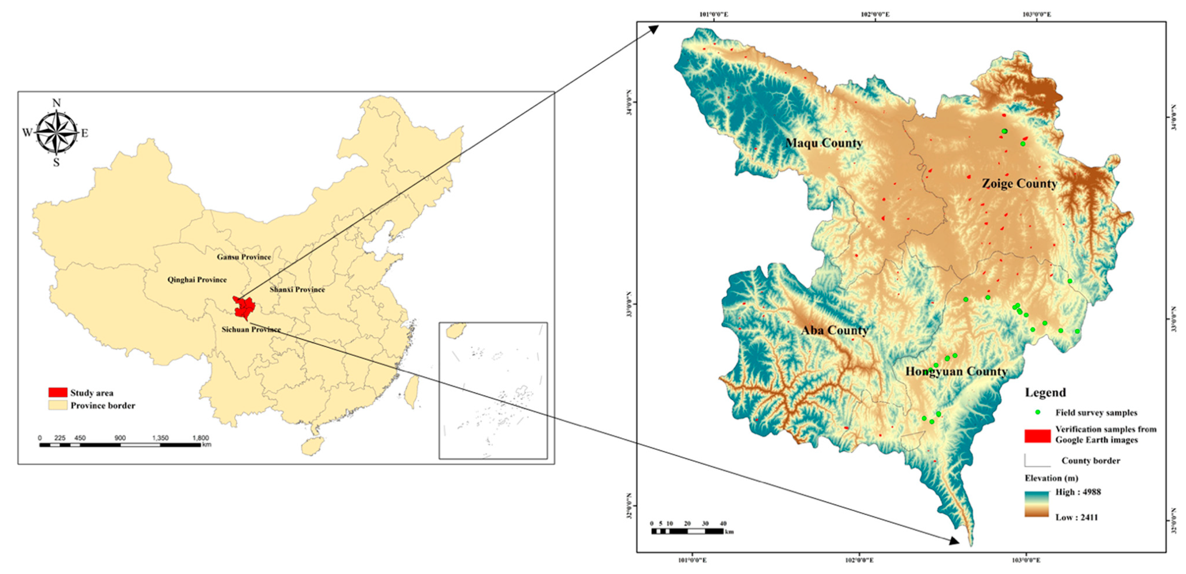
2. Profile of the Study Area

The Zoige Plateau is located at the source area of the Yellow River in the northeastern part of the Qinghai-Tibet Plateau [43,44]. The ecological security of the rich grassland and wetland resources in the Zoige Plateau is related to the social and economic development of the western, Yellow and Yangtze River Basins [42,45,46]. In this study, Zoige, Hongyuan, and Aba counties in Sichuan Province, and Maqu County in Gansu Province were selected as research areas (31°50′–34°30′ N and 100°40′–103°40′ E) (Figure 1). The climate of this region is characterized by a typical humid/semi-humid monsoon climate in the continental cold-temperate zone. The annual precipitation is 400–800 mm and the annual average temperature is 1.6 °C [34]. The study area is rich in tourism resources, including Zoige Wetland Nature Reserve and Huahu scenic area. The process of tourism development has inevitably had an impact on the land use change and landscape pattern.

3. Data and Methods

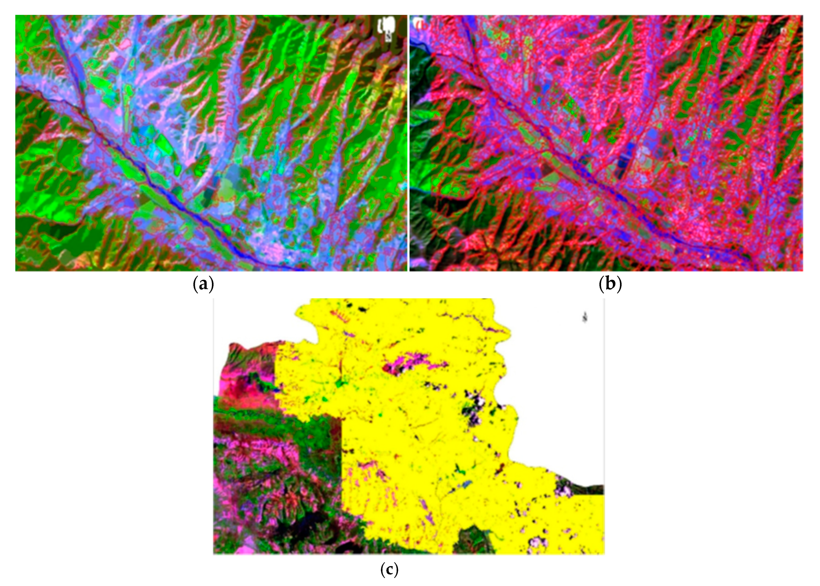
3.1. Data Sources and Processing

The Landsat 8 operational land imager (OLI) has a medium spatial resolution and operates in multiple wavebands, providing an abundance of spectral band information. Landsat 8 OLI was therefore used as the data source for the extraction of land use information from 2015 in the Zoige Plateau. The specific Landsat 8 OLI band information is shown in Table 1. With respect to the data quality and imaging effects, Landsat 8 OLI data for 2015 covering the study area were downloaded from the United States Geological Survey (USGS, http://glovis.usgs.gov/). There were six scenes in total, and the imaging time was from July to November when the growth status of vegetation was good. The specific image information is given in Table 2. Prior to information extraction, Landsat 8 OLI data were processed (e.g., radiation correction, geometric correction and atmospheric correction) to eliminate possible errors. All processing was performed using the ENVI 5.1 software. To realize the long-term dynamic monitoring of land use changes in the Zoige Plateau, the land use data for 2000, 2005, and 2010 were obtained from “Ten-Year Evaluation of National Ecological Environmental Change (2000–2010)” database [47]. These data were generated through visual interpretation using Landsat TM and HJ-1CCD satellite remote sensing images, and independent ground survey samples were used for accuracy evaluation. The average accuracy was >86% [47], which met the study requirements of this area.
Additionally, Google Earth images were used for selecting validation samples. We also conducted a field survey of Zoige and Hongyuan counties in 2016 and got an understanding of the land use status of the area by sample collection and consultation with local experts. The basic geographic data included vector diagrams of the administrative and township divisions in the four counties, which were on the 1:250,000 scale. Projection coordinate information and geographic coordinate information were edited to unify all data for the same coordinate system and thus to avoid data analysis errors caused by inconsistent data coordinates.

3.2. Methods

3.2.1. Land Use Information Extraction by the Object-oriented Method

The whole classification process was completed using the feature extraction module in the ENVI 5.1 software. The detailed processes were as follows.
The first step was to use “Ten-Year Evaluation of National Ecological Environmental Change (2000–2010)” database to determine the seven types of land use in the study area, including forest land, grassland, wetland, water body, farmland, construction land, and unused land (e.g., bare rock, bare soil, and saline-alkali land). The seven land use types represent the ground object information in the study area. In addition, these surface objects showed different colors, shapes, and other features which could be easily distinguished in the Landsat 8 OLI images. For example, wetland was brown and distributed as a combination of grassland and water, while the water body was blue or dark blue.
The second step was to determine a reasonable combination of segmentation level and merge level for high precision information extraction. Through image segmentation and merging, the images were divided into objects. An object represents a combination of pixels with the same or similar attributes within a range. Selecting high-scale image segmentation will produce fewer patches, while a low-level image segmentation will produce more patches. When the threshold is too low, some features will be segmented by wrong images, and a feature may also be divided into many parts. We solved this problem by merging. There were two segmentation algorithms (edge and intensity) and two merging algorithms (full Lambda schedule and fast Lambda) in the Feature Extraction module. We selected the edge algorithm and full Lambda schedule algorithm, respectively. A trial-and-error method was carried out and many repeated experiments of scale combinations between segmentation and merging were adopted to determine the optimum scale. Figure 2a shows the segmented result of optimum segmentation. The segmentation of the image in the study area was considered to be reasonable, with a relatively high internal homogeneity, clear boundary contour, and good representativeness. Figure 2b is the segmented result of over-segmentation. Segmented segments/objects were cracked and the separability between different image objects was low. Figure 2c is the segmented result of under-segmentation, where different kinds of segments/objects were grouped as an object. This meant subsequent information extraction could not be performed correctly. In order to more clearly represent the segmentation effect at the optimal scale, we chose the segmentation images of the representative region for analysis (Figure 3). In Figure 3a, adjacent farmland pixels and construction land pixels could be clustered in an object at this scale, respectively, which demonstrates relatively high internal homogeneity. The region in Figure 3b shows the distribution of grassland, water body, and construction land. The main land use types of the region in Figure 3c are unused land, wetland, and grassland. Grassland and forest land are mainly shown in Figure 3d. On the whole, a good segmentation effect was achieved in both the areas with complex land use types and with a small distribution area of a certain land use type based on Landsat 8 OLI images. The parameter combination at the scale level of 30 and merge level of 60 was determined as the optimum segmentation.
The third step was to establish marks for the seven types of surface features. The object training samples were selected by a visual interpretation of the segmented images. A total of 893 training objects were selected in this study, including grassland (213), forest land (144), wetland (91), water body (55), farmland (30), construction (236), and unused land (124). All attributes including spectral, texture, and spatial attributes of the sample were selected for the following supervised classification in this study.
The fourth step was to use the two classifiers: K-nearest neighbor (KNN) and support vector machine (SVM) for land use classification. The KNN method classifies the image according to the Euclidean distance between the pending number and the elements in the training area in the N-dimensional space [48]. SVM is a supervised learning algorithm that takes the set of training data and marks it as part of a category, then predicts whether the test document is a member of an existing class [48]. The default values in ENVI 5.1 for each parameter of these two classifiers were adopted in this study.
The fifth step was to select the verification samples by visual interpretation using very-high-resolution satellite images available in Google Earth. Because we selected training samples based on polygon units, we also selected the polygonal verification samples in the Google Earth images with nearly four meters resolution in order to match the unit between the two (Figure 1). The precision results were characterized by a confusion matrix. The classification result with the highest accuracy between the method of SVM and of KNN was selected as the final classification result. Considering that there was a certain process and time interval between the changes of land use, it was feasible to verify the classification results of 2015 by using the on-site information of 2016. Therefore, we further verified the results by using the filed survey samples.

3.2.2. Land Use Change Analysis

(1) Comprehensive dynamic degree of land use
The comprehensive dynamic degree of land use refers to the change in the extent of the whole land use type within a certain time range in a study area. It can reflect the comprehensive impact of social and economic activities on land use changes in a region [49]. It is expressed as:
S = ( n = 1 m Δ s i j / s i ) × 1 / t × 100 %
where s i is the total area of land use i at the beginning of monitoring, Δ s i j is the total area of land use i converted into other land uses within the period from the beginning of monitoring to the end of monitoring, and t is the time period.
(2) Dynamic attitude of land use
To quantitatively describe the range, rate, and differences of land use change over a specific time period, the concept of dynamic attitude was introduced by referring to LUCC research. The dynamic attitude of a single land use type expresses the quantitative change of a certain land use type within a certain time range in a certain research area [49], and is expressed as:
L c = ( U b U a ) × U a 1 × T 1 × 100 %
where, L c is the dynamic attitude of the land use type over T years. U a and U b are the area of the land type at the beginning and the end of the study, respectively.
(3) Transfer matrix of land use
The transfer matrix of land use is an analysis method used to describe the transformation between land use types. It can describe the direction of regional land use change and the source and composition of land use types at the end of the study period. It can not only reflect the structure of land use types at the beginning and the end of a study period, but also reflect the transfer and change of land use types during the study period. In this study, the land use types were merged using the dissolve command in ArcGIS10.0 software, and then an overlay analysis was conducted using the intersect command to extract the patches where land use types had changed. The area of these patches was then counted. Finally, the land use transfer matrix was obtained and carried on the spatial display.

3.2.3. Analysis of the Effects of LUCC on Landscape Pattern

LUCC is the main determinant of the landscape spatial pattern and the most direct driving force of changes in the surface landscape pattern. Changes in landscape pattern index were selected to analyze the effects of land use changes on landscape pattern in this study. An analysis of the landscape pattern index generally includes three scales, namely landscape, class, and patch. In this study, 15 landscape pattern indices were selected, which could be divided into four categories, namely area, shape, accumulation and dispersion, and diversity, to represent the landscape pattern of the Zoige Plateau from different perspectives. The landscape pattern index information is presented in Table 3. The specific meaning of, and formula used to calculate each landscape pattern index is given in the description file of the Fragstats 4.2 software [50].
Firstly, we calculated 15 landscape pattern indices of the landscape scale using Fragstats 4.2 software [50] to analyze temporal changes of the overall landscape pattern in the Zoige plateau. Furthermore, we calculated 13 landscape pattern indices of the class scale to see how the changes of different land use types affected the overall landscape pattern. The SHDI and SIDI were not included because they did not have the results of the class scale. The landscape pattern index rate of change for different periods, namely, 2000–2005, 2005–2010, 2010–2015, and 2000–2015, was calculated. Pearson correlation analysis was conducted between the results of the 13 landscape pattern indices rate of the class scale and the corresponding landscape scale results in order to determine the denominating factors. However, the ecological significance of some landscape pattern indices is consistent, so we further analyzed the impact of LUCC on different types of landscape characteristics. The index change rate results of all landscape patterns in one category of each land use type were taken as a whole, and then the Pearson correlation between the landscape pattern at the class and landscape scales was analyzed so as to determine the effects of LUCC on the different categories of the landscape pattern indices. For example, in order to analyze how grassland change affected the area category of landscape, we took the change rates results of four time periods of the three landscape pattern indices (NP, LFI, PD) representing area category of grassland as a whole, and the corresponding results of the landscape scale as a whole, respectively. And then the correlation between two was analyzed. The effects of LUCC on the landscape pattern in different time periods were also determined in this way. The analysis process was completed using the SPSS statistical software.
L a n d R = ( L a n d E L a n d B ) / L a n d B
where, L a n d R is the rate of change of the landscape pattern index, L a n d B is the initial value of the landscape pattern index in the analysis stage, and L a n d E is the later value of the landscape pattern index.

4. Results

4.1. Assessment of Classification Accuracy

The comparison of classification accuracy between SVM and KNN is implemented and shown in Table 4. The results showed that both the overall accuracy (93.2%) and Kappa coefficient (0.889) of SVM were higher than those of the KNN method (57.7% and 0.456). With respect to individual classes, except that the user’s accuracy of water body obtained by KNN method was greater than the result of SVM method, all other SVM classification results were better than KNN. A total of 35 filed survey samples was available (Figure 1), 30 of which were correctly classified in the result of the method of SVM, with a classification accuracy of 85.7%. There were 19 samples of wetland, 16 of which were correctly classified with a classification accuracy of 84.2%, and 3 of which were wrongly classified as water bodies. The land use classification results obtained by combining the object-oriented method and SVM were used to provide land use information for the research area in 2015. However, both SVM and KNN classifications showed lower user accuracy for forest land. Possible reasons for this are explained in the discussion section. In order not to affect later analysis, we manually modified the areas with obvious errors in forest land classification. Combined with land use data, maps of the land use type distribution in the Zoige Plateau in 2000, 2005, 2010, and 2015 were obtained, and the results are shown in Figure 4.

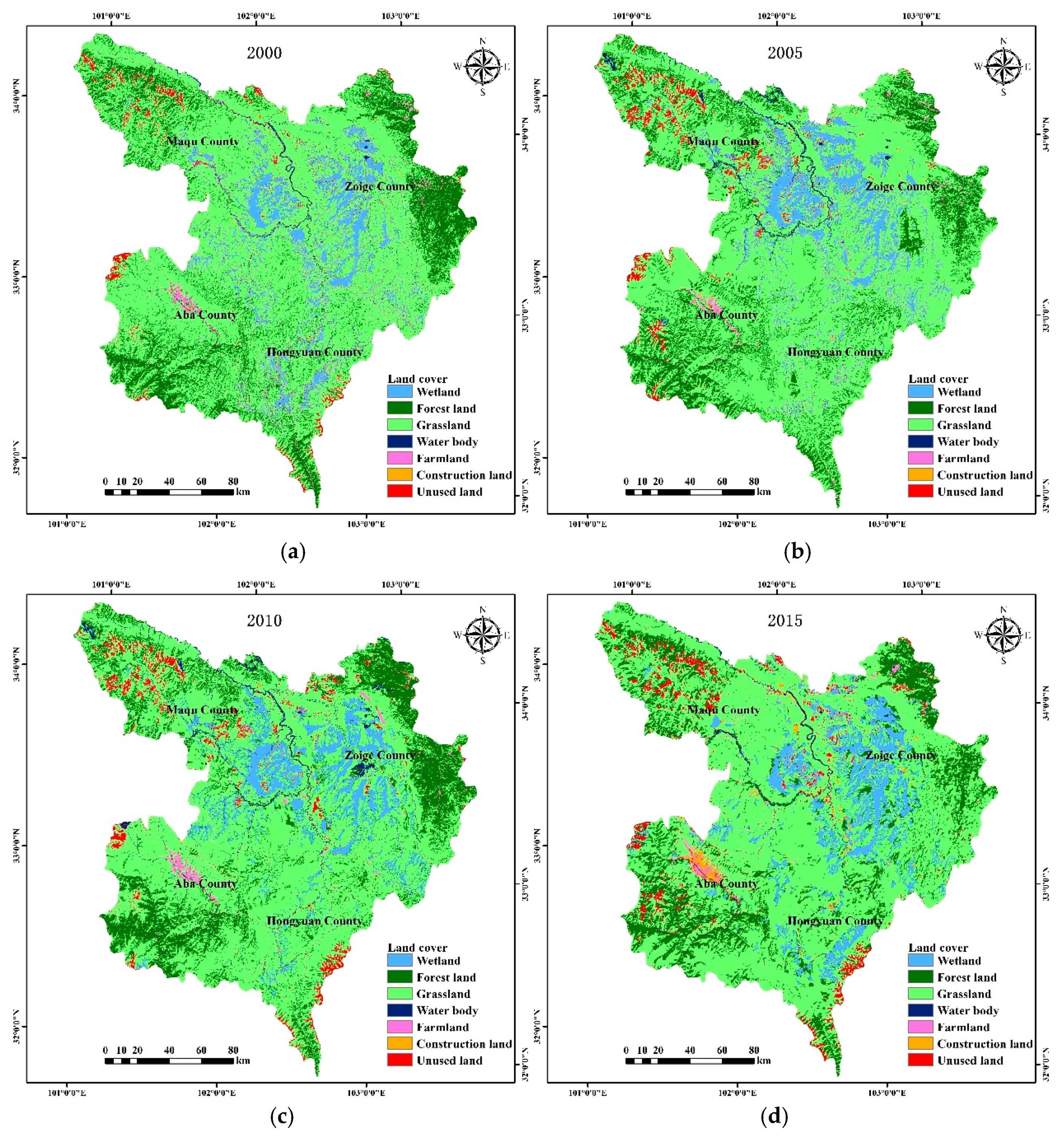
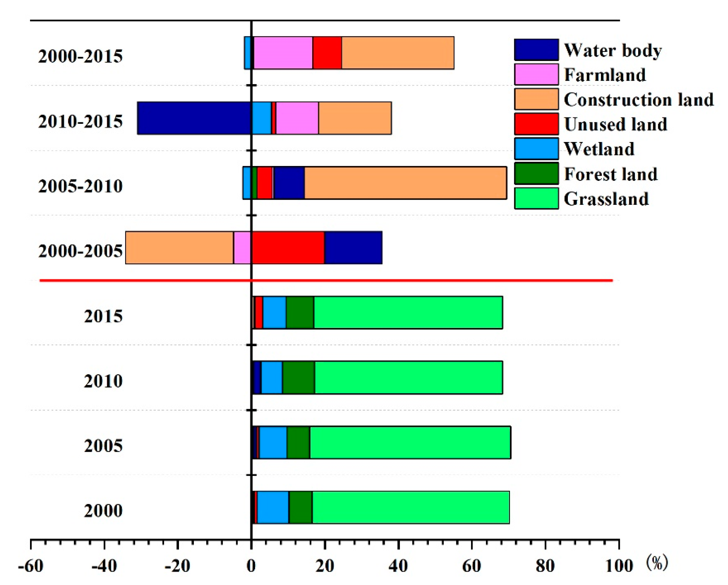
4.2. Characteristics of the Distribution of Land Use Types

Grassland was widely distributed throughout the study area. Forest land was mainly distributed in the east of Zoige County, the southeast of Aba County, and the northwest of Maqu County. There was a belt of wetland distributed throughout the area. Zoige County was the main area where wetland was distributed. Farmland distribution was relatively concentrated, and was mainly distributed in Aba County along the river. The distribution of construction land was relatively scattered, but mostly concentrated along the river. Unutilized land, such as bare rock, was mainly distributed in the northwest of Maqu County and the northeast of Aba County. In recent years, other areas have also developed scattered areas of bare rock.
Figure 5 shows the results of the proportion and rate of change in the proportional area of each land use type from 2000 to 2015. Grassland covered the largest area among the seven land use types, with the proportional area maintained at about 70% from 2000 to 2015. The average ratio of forest land area to total area was 16.8%, displaying a fluctuating trend. Wetland was the third largest land use type in the study area, with an average area ratio of about 9%. Although the area of wetland increased between 2010 and 2015, the area in 2015 was still almost 300 km2 lower than in 2000. The proportional areas of construction land, unused land, and farmland were all relatively small, but there was an increasing trend for all three land use types over the 15-year study period. The area of construction land increased the most in the 15 years, with a proportional area change rate of 223.92%. From the analysis, it was apparent that, over the 15-year study period, the area of construction land, unused land, and farmland increased substantially, while the area of natural ecosystems decreased to varying degrees, among which wetland changed most significantly.

4.3. Characteristics of Land Use Change

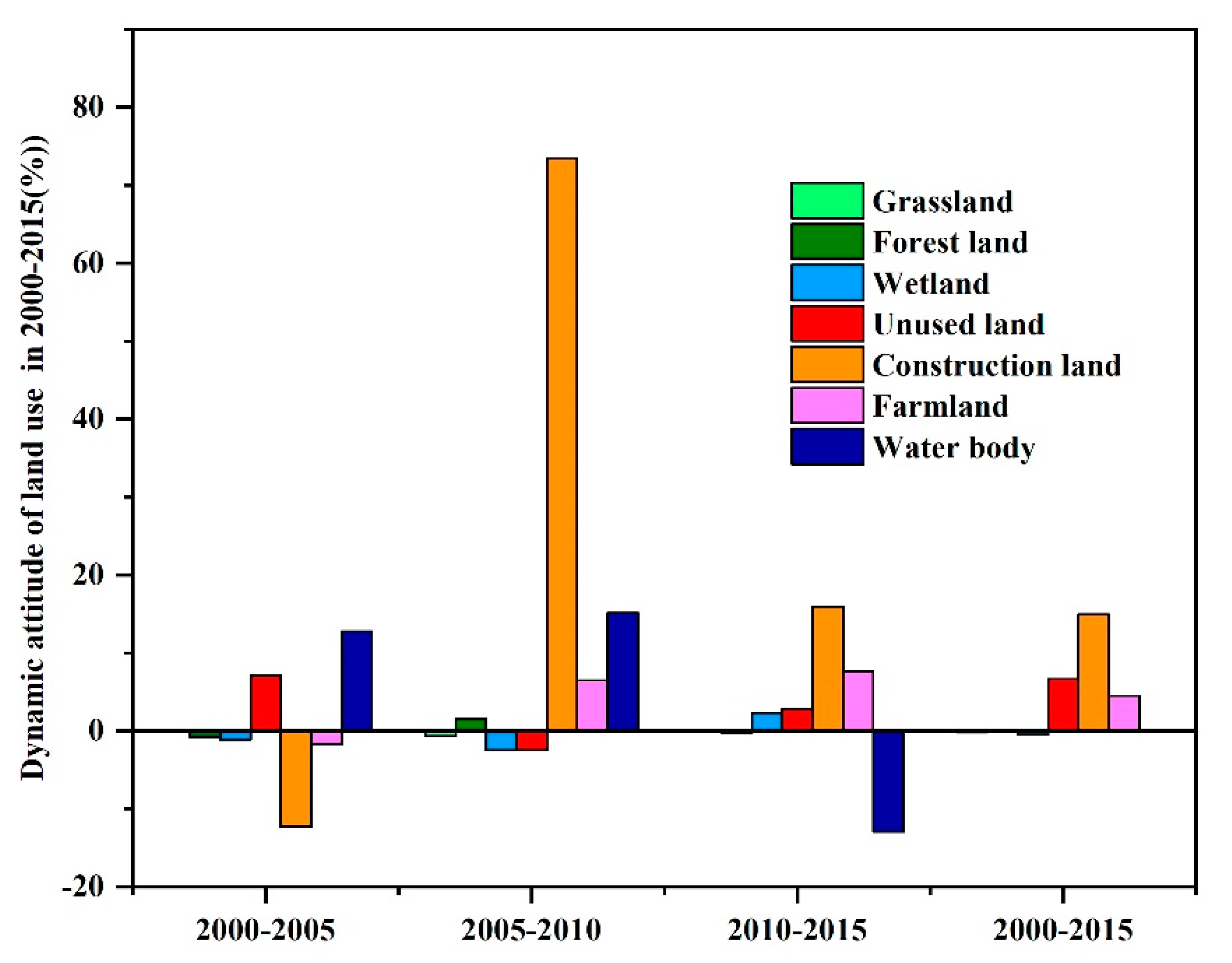
4.3.1. Dynamic Degree of Land Use

The comprehensive dynamic degree of land use values in the Zoige Plateau in the four stages of 2000–2005, 2005–2010, 2010–2015, and 2000–2015 were calculated as 5.27, 4.31, 6.93, and 2.20, respectively. From 2000 to 2015, the comprehensive dynamic degree of land use in the Zoige Plateau was high, and the rate of land use change was increasing, indicating a strong impact of social and economic activities on land use.
The statistical results for the dynamic attitude of each land use type from 2000 to 2015 are shown in Figure 6. The change in the area of grassland remained basically constant over the study period, with little overall change in area. Forest land increased rapidly with an increasing rate of 1.57% during 2005–2010, but with a decreasing rate of 0.20% during 2010–2015. The area of wetlands decreased from 2000 to 2010, and the rate of decrease accelerated with time. The area of unused land increased in both 2000–2005 and 2010–2015, with the rate of increase slowing down from 7.10% during 2000–2005 to 2.81% during 2010–2015. The rate of change of construction land was different, but it was higher than other land use types in the same stage. The trend in the change of farmland area was similar to that of construction land, but the rate of change was faster. The area of water body initially increased, and the growth rate continued to accelerate from 12.75% to 15.15%. In the later stages of the period studied, the area of water body decreased, with a 12.91% reduction rate. From 2000 to 2015, only wetland and grassland decreased in area, with the wetland area decreasing the fastest (−0.51%). Construction land increased the fastest (14.92%), followed by unused land and farmland (6.65% and 4.50%, respectively).

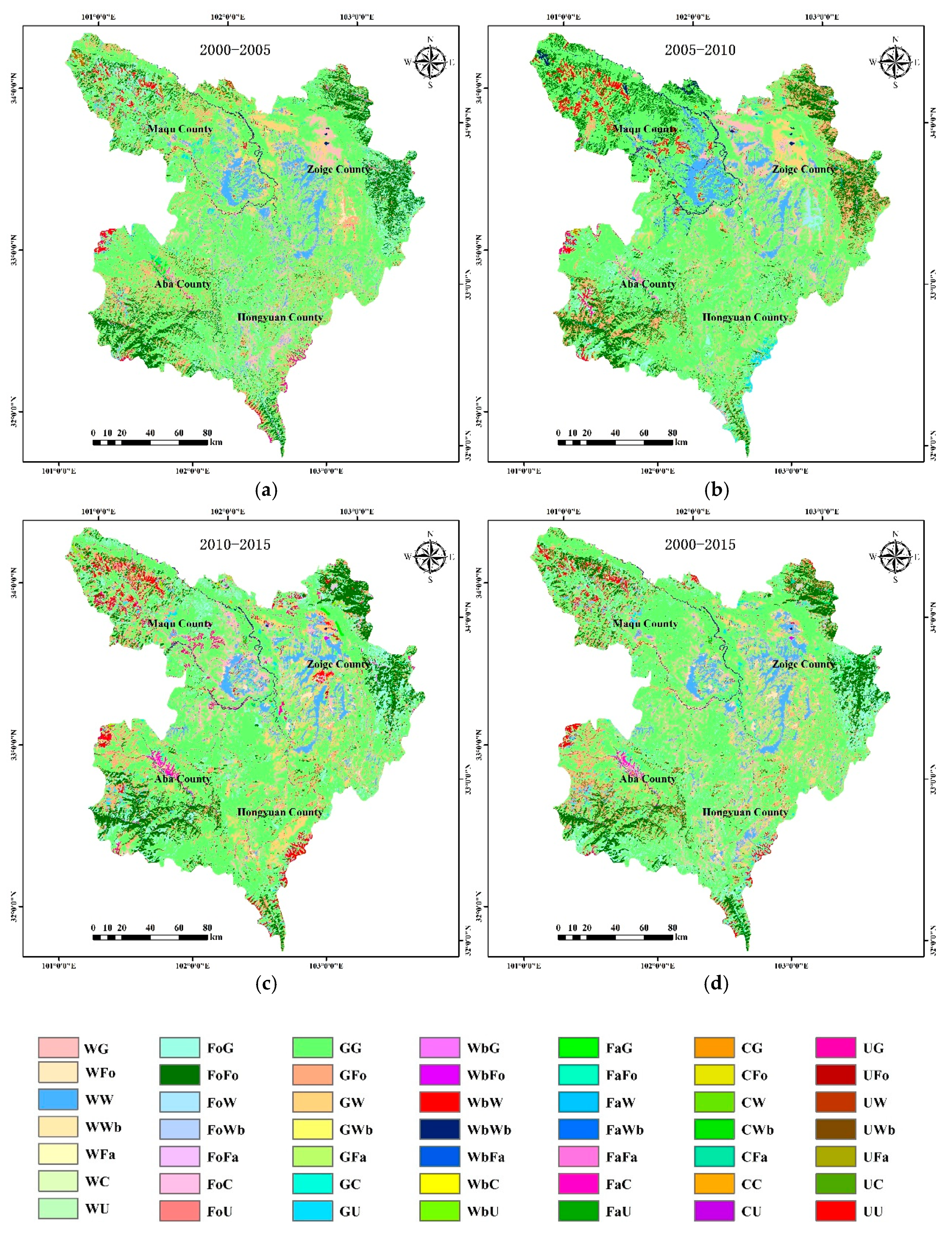
4.3.2. Transfer Matrix of Land Use

From 2000 to 2005 (Figure 7a), 18.44% of grassland was converted to other land types, among which the largest area was converted to forest land (9.60%), followed by wetland (6.11%). Wetland transformation was more obvious, with 49.20% of the total wetland area converted to other uses. Water body, farmland, and construction land all turned out to be grassland to varying degrees, construction land being the most (73.21% of it being turned into grassland). Among the three natural ecosystems, forest land showed the largest difference between the transferred out area and the transferred in area in 2000–2005, and the difference was 255.38 km2.
From 2005 to 2010 (Figure 7b), the trend in the conversion of various land use types was basically the same as that from 2000 to 2005, and the area transferred out was mainly grassland, but there was a decrease in the proportional area of the various land use types that were transferred out. Compared with the period of 2000–2005, the situation regarding the transfer of construction land changed a substantially.
From 2010 to 2015 (Figure 7c), the situation regarding land use changes changed substantially. The proportion of grassland transformed into other land use types increased to 23.60%. The area of wetland converted into other land use types was 1801.88 km2, of which 39.87% was converted into grassland. The transfer of farmland, water body, construction land, and unused land was relatively complex, and a relatively high proportion of the areas of these land use types was converted to other land use types. The difference in the farmland conversion trend was the most obvious, with a reversal from 2005 to 2010. A total of 39.46% of the farmland was converted to construction land, accounting for an area of 100.55 km2.
From 2000 to 2015 (Figure 7d), the transferred out area of grassland was mainly converted into forest land and wetland, accounting for 12.51% and 7.14% of the grassland area, respectively. A total of 57.05% of the wetlands were transferred out, with 39.22% and 15.60% converted into grassland and forest land. The transferred out area of wetland was larger than the transferred in area, thus reducing the total area of wetland by more than 250.00 km2. The conversion of farmland, water body, construction land, and unused land was generally consistent with that from 2010 to 2015, and the transferred in area was larger than the transferred out area, resulting in an increase in the four land use types, among which construction land was the most obvious.

4.4. Analysis of the Effects of LUCC on Landscape Pattern

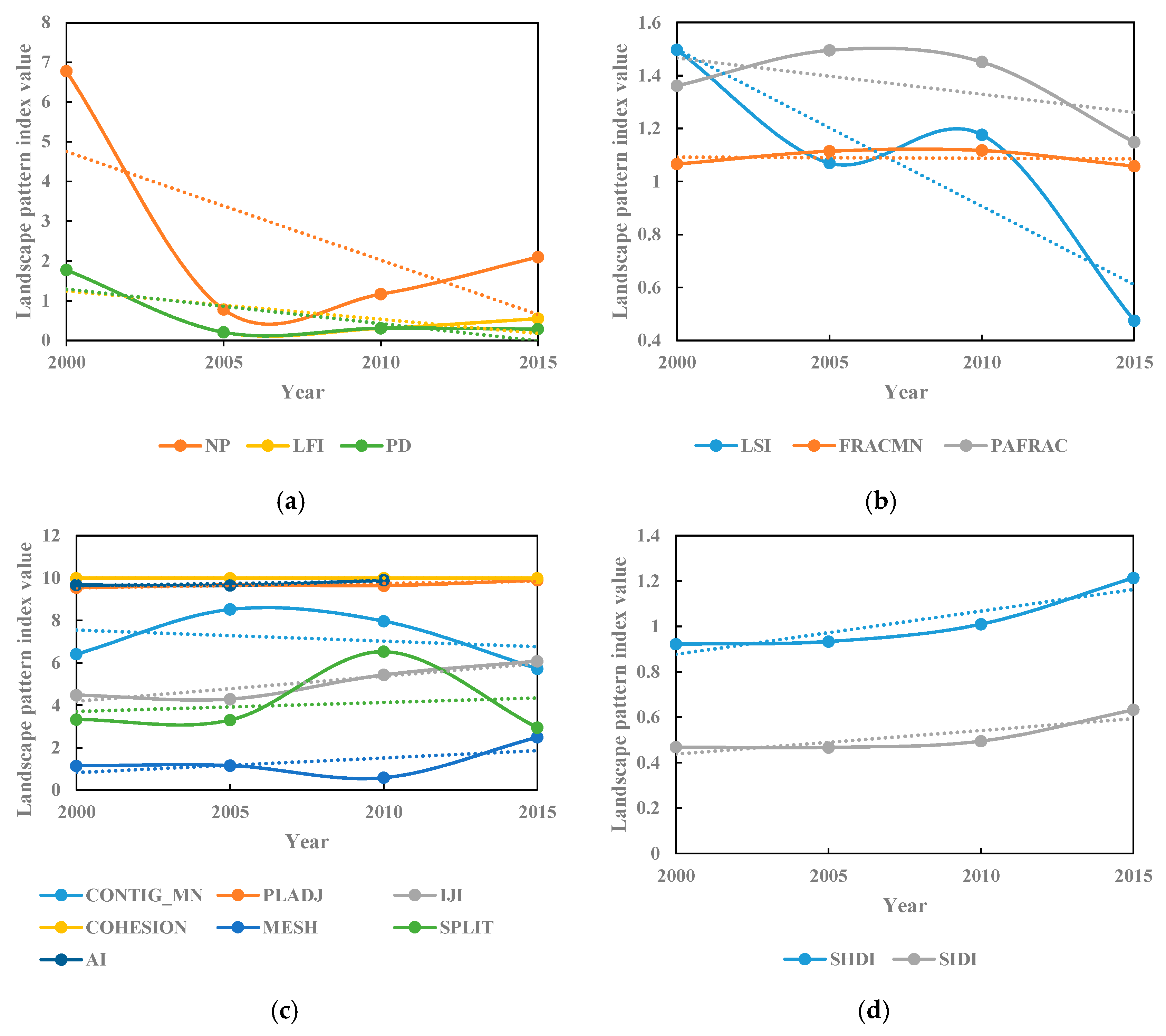
4.4.1. Temporal Changes of the Overall Landscape Pattern

The whole landscape of the Zoige Plateau demonstrated a trend of fragmentation, increasing landscape diversity, and homogenization. The results of indices NP, LFI, and PD showed an overall decreasing trend from 2000 to 2015, but showed an increasing trend from 2005 to 2015 (Figure 8a), indicating that the overall landscape fragmentation increased from 2005 to 2015. In terms of shape category indices (Figure 8b), all the results of LSI, FRAC_MN, and PAFRAC showed an overall trend of decline, meaning that the overall landscape shape in this region tended to be regular and the heterogeneity became smaller. A trend of smaller FRAC_MN indicated that the landscape was increasingly affected by human activities. Most of the indices of accumulation and dispersion category showed an overall increase (Figure 8c), meaning that the overall landscape distribution in this area was scattered and the degree of fragmentation became larger. The diversity indices both showed an increasing trend, showing that the landscape in this region tended to be uniform, and the difference between the dominant landscape elements and other landscape elements decreased (Figure 8d).

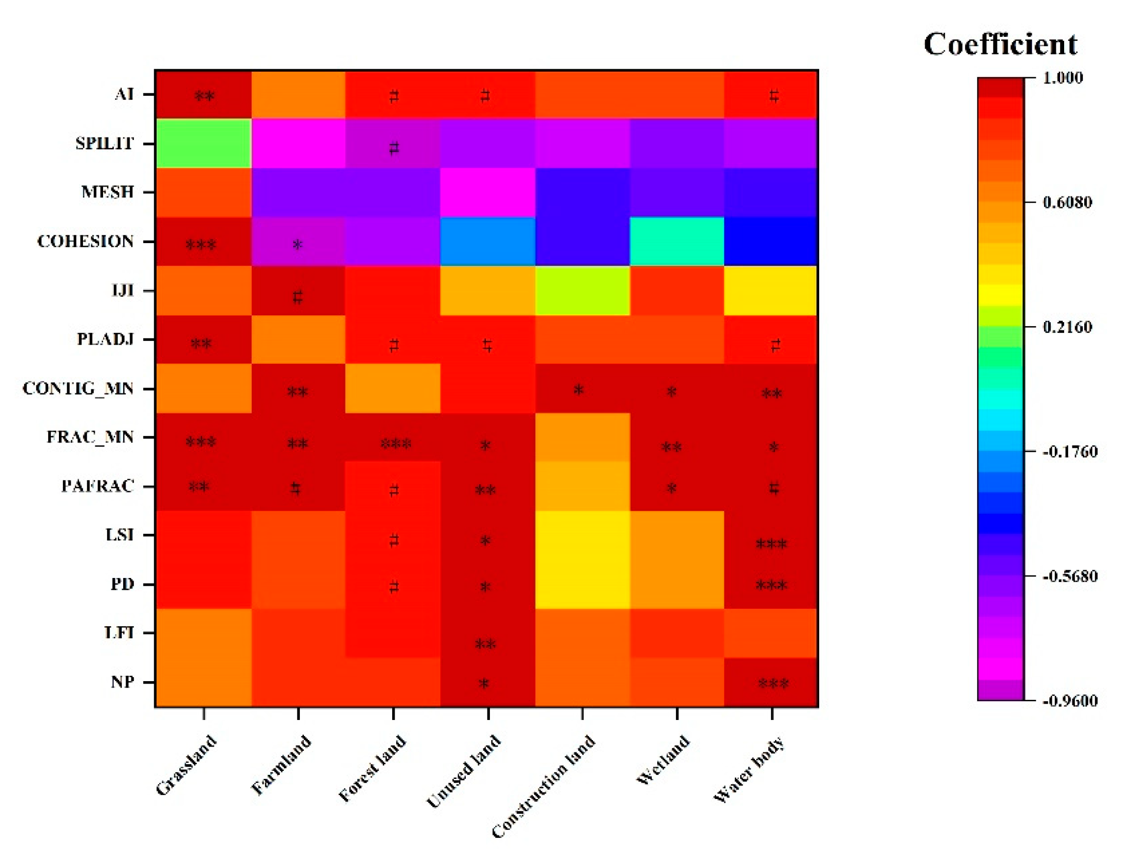
4.4.2. Effects of LUCC on the Landscape Pattern

We analyzed the impact of LUCC on different types of landscape characteristics (area, shape, and accumulation and dispersion) combined with the impact on different landscape pattern index results. The results are shown in Table 5 and Figure 9. The results indicated a significant correlation between the seven land use types and indices of area type at different levels in the study area, mainly due to the chaotic changes in the area of the seven land use types at different stages of the period studied. Among them, the change in the area of unused land had the largest impact on the index of area type, with a correlation coefficient of 0.962 (p < 0.001). This result was consistent in that the unused land had the stronger correlation in the LFI (p < 0.01) (Figure 9). Except for construction land, changes in other land use types could significantly affect the overall landscape shape pattern, among which grassland had the largest impact, with a correlation coefficient of 0.993 (p < 0.001). This was also consistent with the result that grassland was the most important land use type causing changes in PAFRAC and FRAC_MN (Figure 9). The change of forest land was mildly significant (p < 0.10) with the aggregation indices and land use type. The changes of both water body (p < 0.01) and unused land (p < 0.001) showed a strong correlation with the changes of landscape area and shape. These results were also consistent with the effect of water body and unused land on the different landscape pattern indices of area and shape (Figure 9). Although the water body (with a proportional area of only about 1.35% on average) and unused land occupied a small area, they were subject to changes to a large extent during the research stage, which had significant impacts on the landscape pattern.

4.4.3. Effects of LUCC on the Landscape Pattern at Different Time Periods

The effects of land use types at different time periods on the overall landscape pattern were also analyzed. The analysis results are shown in Table 6. From 2000 to 2005, except for water body, all land use types had a significant impact on the changes in the landscape pattern at this stage, among which grassland had the largest impact (0.998, p < 0.001), followed by cultivated land (0.953, p < 0.001) and construction land (0.940, p < 0.001). Water body had the greatest dynamic attitude in this period, but it did not have a great impact on the overall landscape pattern, which indicated that the overall landscape pattern responded comprehensively to changes in all land uses. At this stage, the area of the seven land use types changed substantially, but the influence of the changes in the area of water body was not obvious in the shape, aggregation, and dispersion indices. From 2005 to 2010, the changes in the landscape pattern were mainly affected by the changes in grassland (p < 0.001), farmland (p < 0.05), forest land (p < 0.05), and construction land (p < 0.05). From 2010 to 2015, there was no obvious correlation between changes in the landscape pattern and land use changes. Over the 15-year study period, the influence of farmland, unused land, and construction land was stronger than that of the other land use types, which was also related to the land reclamation projects over this period. It was apparent that land use types occupying a relatively small area could play an important role in changes of the overall landscape pattern.

5. Discussion

(1) The applicability of the object-oriented method based on Landsat 8 OLI for the extraction of land use information in the Zoige Plateau was assessed. Grassland, forest land, and wetland were the three main land use types in this area, and the distribution of these three land use types was relatively concentrated in patches. Therefore, object-oriented analysis could substantially reduce the “salt-and-pepper” noise caused by pixel-based classification. In addition, the shapes of wetland, farmland, and construction land were relatively regular, but showed differences. Based on the object-oriented method, the shape information could be distinguished so as to better classify these three types. Therefore, the land use information for the Zoige Plateau was very accurate, with an overall accuracy of 93.2% and a Kappa coefficient of 0.889, which were higher than in the existing research [53,54]. In addition, many previous studies used visual interpretation to obtain land use information in this region [31,32,34,41], which was time-consuming and laborious, so this study also made a contribution to the automatic acquisition of land use information correctly in this region. However, both SVM and KNN classifications showed lower user accuracy for forest land in this study. The forest land in this area was generally distributed on the mountains with higher elevations, and distributed in belts, which was similar to the distribution shape of wetlands. In addition, the color of wetland was a combination of green vegetation and water, and the forest land was affected by elevation and slope, resulting in no representative difference in color. Both of these two reasons could lead to forest land being misclassified as wetland and water body. The altitude and slope of the object had not been taken into account in the process of the object-oriented method in our study. Therefore, some other ancillary data such as DEM, slope, and aspect could be used and may improve the classification accuracy [17]. Furthermore, the automation and intelligence of image segmentation, scale optimization, and feature space optimization in object–oriented classification would be useful in future studies [17,55].
(2) The results of this study showed that, from 2000 to 2015, the area of land related to production activities had increased greatly, while the area containing natural ecosystems had decreased to varying degrees, among which wetland displayed the most significant change. It is commonly accepted that both climate change and human activities are important factors in the formation and development of wetland degradation [56]. The warmer and drier trend in this area was an indisputable fact [32,42,54,57] that could cause wetland to become drier grassland, or even sandy land [32,42], but the effect was relatively small [54,57,58,59]. Anthropogenic factors were dominant in the loss of wetland. Overgrazing, artificial ditch drainage, land reclamation for agriculture, and peat mining led to irreversible effects on wetland degradation [57,58,59,60]. The statistics showed that over the 15-year study period, the population for Zoige County increased by more than 14,000 people (Figure 10). To meet the material needs of the increasing population, there had been extensive land reclamation, drainage, and dredging of marshland, together with the development of farmland, resulting in the degradation and reduction of grassland and wetland with an increase of farmland and unused land. In view of the importance of wetlands, specific political countermeasures have been carried out, such as the establishment of nature reserves and prohibition of grazing [57]. These measures did have an effect, and the area of wetland increased from 2010 to 2015. However, the protected areas attracted more tourists (Figure 10). Tourism development inevitably had an impact on the natural environment, resulting in the increase of construction land. The warming climate caused glaciers in the Qinghai–Tibetan Plateau to melt, and retreat was a reason for an increased water body area [61]. Furthermore, relevant national eco-environmental protection projects, including the cessation of artificial drainage and building dams to preserve water, are playing an important role in water conservation and supply [57].
(3) We selected a suite of commonly used landscape indices with the aim of capturing detailed information concerning the landscape in this region. The results of indices NP, LFI, and PD of most types of land use increased to varying degrees, among which construction land and farmland were the most obvious during this period. The rate of change of NP of construction land was nearly 1800% from 2010 to 2015. Furthermore, the value of LFI of construction land in each of the four years was the largest among the seven land use types, which suggested that construction land was the dominant type that caused the increased fragmentation of this region. The increasing trend of SHDI and SIDI also illustrated the aggravation of fragmentation in this area from another perspective. The values of LSI, FRAC_MN, and PAFRAC of all seven types showed a decreased trend from 2000 to 2015, revealing a more regular and smaller heterogeneity of landscape shape in this region. We used the correlation analysis method to analyze the effects of land use changes on landscape patterns systematically. Although associations in our results could not prove causality, our multi-angle analysis results suggest that the land use types with a small area have an increasing influence on the whole landscape (Table 5 and Table 6). This study concluded that the effects of land use changes on a relatively small area were intensified over time. One previous study [34] evaluated the changes in ecosystem service values in Zoige Plateau during 1975–2005. They found that due to the expansion of construction land and unused land area, the ecological service value of this area was greatly affected. The value of ecosystem services exhibited an accelerating rate of decrement. These two studies analyzed the impact of land use change in the Zoige Plateau from the perspective of landscape pattern response and ecological service value, respectively. Although the research time interval was different, the change trends of results of these two studies were consistent. Accordingly, our study results also could provide a reference for relevant local government departments to manage and regulate local land use. Although protective measures have had some success, there is still a long way to go to protect and restore the ecosystem functions of the natural systems in the region. How to better balance ecological conservation and economic development is critical [62].

6. Conclusions

Our study analyzed the land use change characteristics of the Zoige Plateau during 2000–2015 and the effects on the regional landscape pattern. Our study showed that it was feasible to extract land use information in the Zoige Plateau by combining the object-oriented method and SVM. Our study revealed that, over the 15–year study period, the area of construction land, unused land, and farmland increased substantially, while grassland, forest land, and wetland decreased to varying degrees, with wetland changing the most significantly. This suggested that human activities have a great impact on the change of land use pattern in this region. The whole landscape of the Zoige Plateau showed a trend of fragmentation, increasing landscape diversity, and homogenization. As a whole, the effects of unused land, farmland, and construction land on the landscape pattern were increasingly stronger than those of the other types, among which farmland had the most significant impact (with correlation coefficient of 0.959, p < 0.001). The changes of unused land and water also made a significant contribution to the change of landscape in different aspects. This suggested that the effects of the changes of land use types with a relatively small area on the overall landscape pattern of the region were intensified over time. Our results suggest that future land use planning of this area could protect natural resources such as wetlands and grasslands, and the impact of relatively small land use types on the whole region should also be considered.

Author Contributions

G.S., X.Y., and Q.Z. conceived the idea and designed the experiments. G.S. and Y.J. performed the experiments. G.S, X.Y., and Y.J. analyzed the data. X.Y., S.L., B.X., and Q.Z. contributed to the discussion of the results and the revision of the article. All authors have read and agreed to the published version of the manuscript.

Funding

This study was supported by the National Key R&D Program of China (2017YFC0506504) and National Natural Science Foundation of China (No. 41571105, 41861019 and 31372354).

Acknowledgments

We acknowledge units such as the grassland management stations in the Sichuan Province of China, which provided extensive support and assistance during the field survey. We are grateful to the reviewers and academic editor for their valuable suggestions and comments.

Conflicts of Interest

The authors declare no conflict of interest.

References

  1. Turner, B.L.; Lambin, E.F.; Reenberg, A. The emergence of land change science for global environmental change and sustainability. Proc. Natl. Acad. Sci. USA 2007, 104, 20666–20671. [Google Scholar] [CrossRef] [PubMed] [Green Version]
  2. Ellis, E.C.; Neerchal, N.; Peng, K.; Xiao, H.S.; Wang, H.; Zhuang, Y.; Li, S.C.; Wu, J.X.; Jiao, J.G.; Ouyang, H.; et al. Estimating long–term changes in China’s village landscapes. Ecosystems 2009, 12, 279–297. [Google Scholar] [CrossRef] [Green Version]
  3. Mendoza, M.E.; Granados, E.L.; Geneletti, D.; Pérez–Salicrup, D.R.; Salinas, V. Analysing land cover and land use change processes at watershed level: A multitemporal study in the Lake Cuitzeo Watershed, Mexico (1975–2003). Appl. Geogr. 2011, 31, 237–250. [Google Scholar] [CrossRef]
  4. Arsanjani, J.J. Dynamic Land Use/Cover Change Simulation: Geosimulation and Multi Agent–Based Modelling; Springer: Berlin/Heidelberg, Germany, 2012. [Google Scholar]
  5. Verburg, P.H.; Steeg, J.V.D.; Veldkamp, A.; Willemen, L. From land cover change to land function dynamics: A major challenge to improve land characterization. J. Environ. Manag. 2009, 90, 1327–1335. [Google Scholar] [CrossRef] [PubMed]
  6. Anderson, R.G.; Canadell, J.G.; Randerson, J.T.; Jackson, R.B.; Hungate, B.A.; Baldocchi, D.D. Biophysical considerations in forestry for climate protection. Front. Ecol. Environ. 2011, 9, 174–182. [Google Scholar] [CrossRef] [Green Version]
  7. Mooney, H.A.; Duraiappah, A.; Larigauderie, A. Evolution of natural and social science interactions in global change research programs. Proc. Natl. Acad. Sci. USA 2013, 110 (Suppl. 1), 3665–3672. [Google Scholar] [CrossRef] [Green Version]
  8. Sterling, S.M.; Ducharne, A.; Polcher, J. The impact of global land–cover change on the terrestrial water cycle. Nat. Clim. Chang. 2012, 3, 385–390. [Google Scholar] [CrossRef]
  9. Tian, H.; Chen, G.; Zhang, C.; Liu, M.; Sun, G.; Chappelka, A. Century–scale responses of ecosystem carbon storage and flux to multiple environmental changes in the southern united states. Ecosystems 2012, 15, 674–694. [Google Scholar] [CrossRef] [Green Version]
  10. Foley, J.A.; DeFries, R.; Asner, G.P.; Barford, C.; Bonan, G.; Carpenter, S.R.; Chapin, F.S.; Coe, M.T.; Daily, G.C.; Gibbs, H.K.; et al. Global consequences of land use. Science 2005, 309, 570–574. [Google Scholar] [CrossRef] [Green Version]
  11. Alemayehu, F.; Taha, N.; Nyssen, J.; Girma, A.; Zenebe, A.; Behailu, M. The impacts of watershed management on land use and land cover dynamics in Eastern Tigray (Ethiopia). Resour. Conserv. Recycl. 2009, 53, 192–198. [Google Scholar] [CrossRef]
  12. Zhang, F.; Tashpolat, T.; Kung, H.T.; Ding, J. The change of land use/cover and characteristics of landscape pattern in arid areas oasis: An application in Jinghe, Xinjiang. Geospat. Inf. Sci. 2010, 13, 174–185. [Google Scholar] [CrossRef] [Green Version]
  13. Jin, S.M.; Yang, L.M.; Danielson, P.; Homer, C.; Fry, J.; Xian, G. A comprehensive change detection method for updating the national land cover database to circa 2011. Remote Sens. Environ. 2013, 132, 159–175. [Google Scholar] [CrossRef] [Green Version]
  14. Li, Z.Y.; Liu, X.H.; Niu, T.L.; Kejia, D.; Zhou, Q.P.; Ma, T.X.; Gao, Y.Y. Ecological restorationand its effects on a regional climate: The source region of the Yellow River, China. Environ. Sci. Technol. 2015, 49, 5897–5904. [Google Scholar] [CrossRef] [PubMed]
  15. Song, X.P.; Hansen, M.C.; Stehman, S.V.; Potapov, P.V.; Alexandra, T.; Vermote, E.F.; Townshend, J.R. Global land change from 1982 to 2016. Nature 2018, 560, 639–643. [Google Scholar] [CrossRef]
  16. Baatz, M.; Arini, N.; Schape, A.; Binnig, G.; Linssen, B. Object–oriented image analysis for high content screening: Detailed quantification of cells and sub cellular structures with the Cellenger software. Int. Soc. Anal. Cytol. 2006, 69, 652–658. [Google Scholar] [CrossRef]
  17. Hu, Q.; Wu, W.B.; Xia, T.; Yu, Q.Y.; Yang, P.; Li, Z.G.; Song, Q. Exploring the use of Google Earth imagery and object–based methods in land use/cover mapping. Remote Sens. 2013, 5, 6026–6042. [Google Scholar] [CrossRef] [Green Version]
  18. Keyport, R.N.; Oommen, T.; Martha, T.R.; Sajinkumar, K.S.; Gierke, J.S. A comparative analysis of pixel– and object–based detection of landslides from very high–resolution images. Int. J. Appl. Earth Obs. Geoinf. 2018, 64, 1–11. [Google Scholar] [CrossRef]
  19. Stumpf, A.; Kerle, N. Object–oriented mapping of landslides using random forests. Remote Sens. Environ. 2011, 115, 2564–2577. [Google Scholar] [CrossRef]
  20. Forman, R.T.T.; Godron, M. Landscape Ecology; John Wiley & Sons: New York, NY, USA, 1986. [Google Scholar]
  21. Wu, J.G.; Hobbs, R. Key issues and research priorities in landscape ecology: An idiosyncratic synthesis. Landscape Ecol. 2002, 17, 355–365. [Google Scholar] [CrossRef]
  22. Dale, V.H.; Brown, S.; Haeuber, R.; Hobbs, N.T.; Huntly, N.; Naiman, R.J.; Riebsame, W.E.; Turner, M.G.; Valone, T. Ecological principles and guidelines for managing the use of land. Ecol. Appl. 2000, 10, 639–670. [Google Scholar] [CrossRef] [Green Version]
  23. Zhang, Y.; Wang, G.X.; Wang, Y.B. Changes in alpine wetland ecosystems of the Qinghai–Tibetan Plateau from 1967 to 2004. Environ. Monit. Assess. 2011, 180, 189–199. [Google Scholar] [CrossRef] [PubMed] [Green Version]
  24. Turner, M.G.; Gardner, R.H. Landscape Ecology in Theory and Practice: Pattern and Process, 2nd ed.; Springer: Berlin/Heidelberg, Germany, 2015. [Google Scholar]
  25. Wu, J.G. Landscape Ecology: Pattern, Process, Scale and Hierarchy; Higher Education Press: Beijing, China, 2007. (In Chinese) [Google Scholar]
  26. Turner, M.G.; Gardner, R.H. Quantitative Methods in Landscape Ecology; Springer: Berlin/Heidelberg, Germany, 1991. [Google Scholar]
  27. Turner, M.G.; O’Neill, R.V.; Gardner, R.H.; Milne, B.T. Effects of changing spatial scale on the analysis of landscape pattern. Landsc. Ecol. 1989, 3, 153–162. [Google Scholar] [CrossRef]
  28. Pickett, S.T.A.; White, P.S. The ecology of natural disturbance and patch dynamics. Science 1985, 230, 434–435. [Google Scholar]
  29. Li, H.B.; Wu, J.G. Use and misuse of landscape indices. Landsc. Ecol. 2004, 19, 389–399. [Google Scholar] [CrossRef] [Green Version]
  30. Li, X.D.; Du, Y.; Ling, F.; Wu, S.J.; Feng, Q. Using a sub–pixel mapping model to improve the accuracy of landscape pattern indices. Ecol. Indic. 2011, 11, 1160–1170. [Google Scholar] [CrossRef]
  31. Bai, J.H.; Ouyang, H.; Cui, B.S.; Wang, Q.G.; Chen, H. Changes in landscape pattern of alpine wetlands on the Zoige Plateau in the past four decades. Acta Ecol. Sin. 2008, 28, 2245–2252. [Google Scholar]
  32. Bai, J.H.; Wang, J.J.; Zhao, Q.Q.; Hua, O.; Wei, D.; Li, A.N. Landscape pattern evolution processes of alpine wetlands and their driving factors in the Zoige Plateau of China. J. Mt. Sci. 2013, 10, 54–67. [Google Scholar] [CrossRef]
  33. Zubaida, M.; Xia, J.X.; Polat, M.; Zhang, R. Land use and landscape pattern changes in the middle reaches of the Keriya River. Acta Ecol. Sin. 2019, 39, 1–9. (In Chinese) [Google Scholar]
  34. Li, J.C.; Wang, W.L.; Hu, G.Y.; Wei, Z.H. Changes in ecosystem service values in Zoige plateau, china. Agric. Ecosyst. Environ. 2010, 139, 766–770. [Google Scholar] [CrossRef]
  35. Li, Z.Y.; Wu, W.Z.; Liu, X.H.; Fath, B.D.; Sun, H.L.; Liu, X.C.; Xiao, X.R.; Cao, J. Land use/cover change and regional climate change in an arid grassland ecosystem of Inner Mongolia, China. Ecol. Model. 2017, 353, 86–94. [Google Scholar] [CrossRef]
  36. Wetland China. The Report on the Second National Wetland Resources Survey (2009–2013). 2014. Available online: http://www.shidi.org (accessed on 20 April 2018).
  37. Huo, L.L.; Chen, Z.K.; Zou, Y.C.; Lu, X.G.; Guo, J.W.; Tang, X.G. Effect of Zoige alpine wetland degradation on the density and fractions of soil organic carbon. Ecol. Eng. 2013, 51, 287–295. [Google Scholar] [CrossRef]
  38. Hu, G.Y.; Dong, Z.B.; Lu, J.F.; Yan, C.Z. Driving forces of land use and land cover change (LUCC) in the Zoige Wetland, Qinghai–Tibetan Plateau. Sci. Cold Arid Reg. 2012, 4, 422–430. [Google Scholar]
  39. Zhang, W.J.; Lu, Q.F.; Song, K.C.; Qin, G.H.; Wang, Y.; Wang, X.; Li, H.X.; Li, J.; Liu, G.D.; Li, H. Remotely sensing the ecological influences of ditches in Zoige Peatland, eastern Tibetan Plateau. Int. J. Remote Sens. 2014, 35, 5186–5197. [Google Scholar] [CrossRef]
  40. Zhang, W.J.; Yi, Y.H.; Song, K.C.; Kimball, J.S.; Lu, Q.F. Hydrological response of alpine wetlands to climate warming in the eastern Tibetan Plateau. Remote Sens. 2016, 8, 336. [Google Scholar] [CrossRef] [Green Version]
  41. Jiang, P.H.; Cheng, L.; Li, M.C.; Zhao, R.F.; Duan, Y.W. Impacts of LUCC on soil properties in the riparian zones of desert oasis with remote sensing data: A case study of the middle Heihe River basin, China. Sci. Total Environ. 2015, 506–507, 259–271. [Google Scholar] [CrossRef] [PubMed]
  42. Pang, A.P.; Li, C.H.; Wang, X.; Hu, J. Land use/cover change in response to driving forces of Zoige County, China. Procedia Environ. Sci. 2010, 2, 1074–1082. [Google Scholar] [CrossRef] [Green Version]
  43. Xiang, S.; Guo, R.Q.; Ning, W.; Sun, S.C.; Qin, P.; Mitsch, W.J. Current status and future prospects of Zoige marsh in Eastern Qinghai–Tibet Plateau. Ecol. Eng. 2009, 35, 553–562. [Google Scholar] [CrossRef]
  44. Dong, Z.B.; Hu, G.Y.; Yan, C.Z.; Wang, W.L.; Lu, J.F. Aeolian desertification and its causes in the Zoige Plateau of China’s Qinghai–Tibetan Plateau. Environ. Earth Sci. 2010, 59, 1731–1740. [Google Scholar] [CrossRef]
  45. Zhang, B.L.; Zhang, S.M.; Zhou, W.C. Muti–source data–based remote sensing auto–survey of land use in Ruoergai wetland. Soils 2008, 40, 283–287. [Google Scholar]
  46. Shen, G.; Xu, B.; Jin, Y.X.; Chen, S.; Zhang, W.B.; Guo, J.; Liu, H.; Zhang, Y.J.; Yang, X.C. Advances in studies of wetlands in Zoige Plateau. Geogr. Inf. Sci. 2016, 32, 76–82. (In Chinese) [Google Scholar]
  47. Ouyang, Z.Y.; Zheng, H.; Xiao, Y.; Polasky, S.; Liu, J.G.; Xu, W.H.; Wang, Q.; Zhang, L.; Xiao, Y.; Rao, E.M.; et al. Improvements in ecosystem services from investments in natural capital. Science 2016, 352, 1455–1459. [Google Scholar] [CrossRef] [PubMed]
  48. Pratama, B.Y.; Sarno, R. Personality classification based on Twitter text using Naive Bayes, KNN and SVM. In Proceedings of the 2015 International Conference on Data & Software Engineering, Yogyakarta, Indonesia, 25–26 November 2015; IEEE: Piscataway, NJ, USA, 2015. [Google Scholar]
  49. Wang, X.L.; Bao, Y.H. Study on the methods of land use dynamic change research. Prog. Geogr. 1999, 18, 81–87. (In Chinese) [Google Scholar]
  50. McGarigal, K.; Cushman, S.A.; Ene, E. FRAGSTATS v4: Spatial Pattern Analysis Program for Categorical and Continuous Maps. Computer Software Program Produced by the Authors at the University of Massachusetts, Amherst. 2012. Available online: http://www.umass.edu/landeco/research/fragstats/fragstats.html (accessed on 20 May 2019).
  51. McGarigal, K.; Marks, B.J. FRAGSTATS: Spatial Pattern Analysis Program for Quantifying Landscape Structure; General Technical Report; U.S. Department of Agriculture, Forest Service, Pacific Northwest Research Station: Portland, OR, USA, 1995.
  52. Plexida, S.G.; Sfougaris, A.I.; Ispikoudis, I.P.; Papanastasis, V.P. Selecting landscape metrics as indicators of spatial heterogeneity—A comparison among Greek landscapes. Int. J. Appl. Earth Obs. Geoinf. 2014, 26, 26–35. [Google Scholar] [CrossRef]
  53. Zheng, Y.M.; Niu, Z.G.; Gong, P.; Li, M.N.; Hu, L.L.; Wang, L.; Yang, Y.X.; Gu, H.J.; Mu, J.R.; Dou, G.J.; et al. A method for alpine wetland delineation and features of border: Zoigê Plateau, China. Chin. Geogr. Sci. 2017, 27, 784–799. [Google Scholar] [CrossRef] [Green Version]
  54. Li, Z.W.; Gao, P.; Hu, X.Y.; Yi, Y.J.; Pan, B.Z.; You, Y.C. Coupled impact of decadal precipitation and evapotranspiration on peatland degradation in the Zoige basin, china. Phys. Geogr. 2019, 6, 1–24. [Google Scholar] [CrossRef]
  55. Cheng, J.H.; Bo, Y.C.; Zhu, Y.X.; Ji, X.L. A novel method for assessing the segmentation quality of high–spatial resolution remote–sensing images. Int. J. Remote Sens. 2014, 35, 3816–3839. [Google Scholar] [CrossRef]
  56. Hu, S.J.; Niu, Z.G.; Chen, Y.F.; Li, L.F.; Zhang, H.Y. Global wetlands: Potential distribution, wetland loss, and status. Sci. Total Environ. 2017, 586, 319–327. [Google Scholar] [CrossRef]
  57. Hu, G.Y.; Dong, Z.B.; Lu, J.F.; Yan, C.Z. The developmental trend and influencing factors of aeolian desertification in the Zoige Basin, eastern Qinghai–Tibet Plateau. Aeolian Res. 2015, 19, 275–281. [Google Scholar] [CrossRef]
  58. Yu, K.F.; Lehmkuhl, F.; Folk, D. Quantifying land degradation in the Zoige Basin, NE Tibetan Plateau using satellite remote sensing data. J. Mt. Sci. 2017, 14, 77–93. [Google Scholar] [CrossRef]
  59. You, Y.C.; Li, Z.W.; Li, X.L. Land cover change in Zoige Plateau during 1990–2011. Adv. Sci. Technol. Water Resour. 2018, 38, 62–69. (In Chinese) [Google Scholar]
  60. Zhang, X.H.; Liu, H.Y.; Baker, C.; Graham, S. Restoration approaches used for degraded peatlands in Ruoergai (Zoige), Tibetan Plateau, China, for sustainable land management. Ecol. Eng. 2012, 38, 86–92. [Google Scholar] [CrossRef]
  61. Xu, W.H.; Fan, X.Y.; Ma, J.K.; Pimm, S.L.; Kong, L.Q.; Zeng, Y.; Li, X.S.; Xiao, Y.; Zheng, H.; Liu, J.G.; et al. Hidden loss of wetlands in China. Curr. Biol. 2019, 29, 3065–3071. [Google Scholar] [CrossRef] [PubMed] [Green Version]
  62. Xu, W.H.; Pimm, S.L.; Du, A.; Su, Y.; Fan, X.Y.; An, L.; Liu, J.G.; Ouyang, Z.Y. Transforming protected area management in China. Trends Ecol. Evol. 2019, 34, 762–766. [Google Scholar] [CrossRef] [PubMed] [Green Version]
Figure 1. Location of the study area.
Remotesensing 12 00014 g001
Figure 2. Comparison of segmentation results at different scales based on Landsat 8 OLI. (a) Optimum segmentation. The red line represents the object border. (b) Over-segmentation. The red line represents the object border. (c) Under-segmentation. The yellow areas in Figure c represent one segmented object, which contains mixed pixels.
Remotesensing 12 00014 g002
Figure 3. Image segmentation sketch diagrams of representative areas based on Landsat 8 OLI. The red line represents the object border. (a) Farmland, construction land, and grassland; (b) grassland, water body, and construction land; (c) unused land, wetland, and grassland; (d) grassland and forest land.
Remotesensing 12 00014 g003
Figure 4. Land use results for the Zoige Plateau in 2000–2015. (a): Land use map in 2000; (b): Land use map in 2005; (c): Land use map in 2010; (d): Land use map in 2015. Land use data for 2000, 2005, and 2010 are obtained from “Ten-Year Evaluation of National Ecological Environmental Change (2000–2010)” database [47]. The data for 2015 is the classification result based on the object-oriented method.
Remotesensing 12 00014 g004
Figure 5. The upper part of the solid red line shows the results of rate of change in the proportional area of different land use in the Zoige Plateau in 2000–2015. The rate of change in the proportional area refers to the rate of proportion change of the land use type in two time periods. The below part of the solid red line show the results of land use proportional area of the Zoige Plateau in 2000–2015.
Remotesensing 12 00014 g005
Figure 6. Dynamic attitude of land use in the Zoige Plateau in 2000–2015 (%).
Remotesensing 12 00014 g006
Figure 7. Distribution of land use conversion in the Zoige Plateau. (a): Distribution of land use conversion during 2000–2005; (b): Distribution of land use conversion during 2005–2010; (c): Distribution of land use conversion during 2010–2015; (d): Distribution of land use conversion during 2000–2015. In the legend, W stands for wetland, G for grassland, Fo for forest land, Wb for water body, Fa for farmland, C for construction land and U for unused land, respectively. WG means that the wetlands are converted into grasslands. Other annotations also indicate such a transformation relationship.
Remotesensing 12 00014 g007
Figure 8. Temporal changes of 15 different landscape pattern indices of landscape scale. (a) Landscape pattern indices of the area category; (b) landscape pattern indices of the shape category; (c) landscape pattern indices of the accumulation and dispersion category; (d) Landscape pattern indices of the diversity category. Many of the landscape pattern indices results in the graphs have been processed to facilitate the display of change trends. For example, the values of NP were reduced 10,000-fold.
Remotesensing 12 00014 g008
Figure 9. Correlation results between the landscape pattern indices of the class scale and the corresponding landscape scale results. The ordinate represents 13 landscape pattern indices results of the landscape scale, and the abscissa represents landscape pattern indices results of different land use type. Different colors indicate the correlation results between the 13 landscape pattern indices rate of the class scale and the corresponding landscape scale results. *** p < 0.001, ** p < 0.01, * p < 0.05, # p < 0.10.
Remotesensing 12 00014 g009
Figure 10. Statistical data of Zoige County in 2000–2015. The data were obtained through the local bureau of statistics.
Remotesensing 12 00014 g010
Table 1. Spectral bands of Landsat 8 operational land imager (OLI) sensor.
BandsWavelength (μm)Resolution (m)
Band 1-Coastal0.433–0.45330
Band 2-Blue0.450–0.51530
Band 3-Green0.525–0.60030
Band 4-Red0.630–0.68030
Band 5-NIR (Near Infrared)0.845–0.88530
Band 6-SWIR (Short-wave infrared) 1 1.560–1.65130
Band 7-SWIR22.100–2.30030
Band 8-Pan0.500–0.68015
Band 9-Cirrus1.360–1.39030
Table 2. Basic details of the Landsat 8 OLI images.
TypePath RowTimeCloud Cover (%)
OLI130037201507068.12
OLI131036201507291.9
OLI131037201507296.97
OLI131038201511020.74
OLI132036201509220.85
OLI132037201509222
Table 3. Landscape pattern index information [50,51,52].
CategoryIndex NameDescription
AreaNumber of patches (NP)Total number of patch.
Landscape fragmentation index (LFI)The ratio of number of patches and the area of corresponding the landscape.
Patch density (PD)Number of patches per unit area.
ShapeLandscape shape index (LSI)A standardized measure of patch compactness that adjusts for the size of the patch.
Perimeter area fractal dimension (PAFRAC)Non-randomness or degree of aggregation for different patches.
Mean fractal dimension (FRAC_MN)The shape complexity of patches, which approaches 1 for shapes with simple perimeters and 2 for complex shapes.
Accumulation and dispersionMean patch contiguity index (CONTIG_MN)It equals the average contiguity value for the cells in a patch.
Proportion of like adjacency (PLADJ)It equals the number of like adjacencies involving the focal class, divided by the total number of cell adjacencies involving the focal class; multiplied by 100 (to convert to a percentage). It measures the degree of aggregation of the focal patch type.
Interspersion and juxtaposition index (IJI)The measurement of evenness of patch adjacencies and the degree of intermixing of patch types.
Patch cohesion index (COHESION)It is proportional to the area-weighted mean perimeter-area ratio divided by the area-weighted mean patch shape index.
Effective mesh size (MESH)The ratio of square of summed patch areas and the total area. It expresses the fragmentation independent of the extent of the studied landscape.
Splitting index (SPILIT)The number of patches obtained with subdividing the landscape into equal-sized patches based on the effective mesh size.
Aggregation index (AI)The ratio of the observed number of like adjacencies and the maximum possible number of like adjacencies given the proportion of the landscape comprised of each patch type.
DiversityShannon’s diversity index (SHDI)Uncertainties and landscape heterogeneity of patches.
Simpson’s diversity index (SIDI)It equals 1 minus the sum, across all patch types, of the proportional abundance of each patch type squared
Table 4. The comparison of classification accuracy between SVM and KNN.
SVMKNN
User’s Accuracy (%)Producer’s Accuracy (%)User’s Accuracy (%)Producer’s Accuracy (%)
Grassland99.5498.6496.9434.75
Farmland91.6299.5257.5379.64
Forest land42.1910033.7249.45
Unused land99.7710078.1685.82
Construction land10010069.7856.14
Wetland10086.5295.2788.35
Water body70.9510098.3470.87
Overall accuracy (%): SVM = 93.2, KNN = 57.7
Kappa: SVM = 0.889, KNN = 0.456
Table 5. Results of effects of LUCC on the different categories of the landscape pattern indices.
CategoryGrasslandFarmlandForest LandUnused LandConstruction LandWetlandWater Body
Area0.706 *0.820 ***0.873 **0.962 ***0.621 *0.766 **0.768 **
Shape0.993 ***0.608 *0.966 ***0.919 ***0.3860.863 ***0.816 **
Accumulation and dispersion0.153−0.274−0.360 #−0.2850.023−0.190−0.230
*** p < 0.001, ** p < 0.01, * p < 0.05, # p < 0.10
Table 6. Results of the response of the landscape pattern indexes at different time periods.
GrasslandFarmlandForest LandUnused LandConstruction LandWetlandWater Body
2000–20050.998 ***0.953 ***0.561 *0.727 **0.940 ***0.788 **0.268
2005–20100.842 ***−0.613 *−0.587 *0.030−0.570 *0.4280.288
2010–20150.328−0.011−0.325−0.2860.1640.086−0.222
2000–20150.3630.959 ***0.1580.833 ***0.752 **0.681 **0.154
*** p < 0.001, ** p < 0.01, * p < 0.05, # p < 0.10

