Author Contributions
Conceptualization, H.Y.; methodology, Y.A.; software, Y.A., R.K. and H.Y.; validation, Y.A., R.K., K.O., and H.Y.; formal analysis, Y.A.; investigation, Y.A.; resources, H.Y.; data curation, Y.A.; writing—original draft preparation, Y.A.; writing—review and editing, K.O. and H.Y.; visualization, Y.A. and R.K.; supervision, K.O. and H.Y.; project administration, H.Y.; and funding acquisition, Y.A. and H.Y.
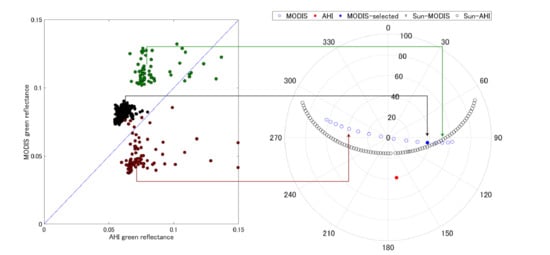
Figure 1.
Scatter plot (left) of the TOC reflectances observed by AHI and MODIS, with the corresponding green bands. The data were extracted from our test site over the Kochi Forest during the period between 12 and 14 May 2016. The observation pairs over the three days are indicated by different colors. The data acquisition times of the three groups of reflectance pairs were nearly identical. (right) A polar plot of the illumination and view angles. Sixteen variations in the MODIS view angles (11–26 May 2016) are also plotted.
Figure 2.
Angular conditions of the sun, MODIS, and AHI for the SZM method (a) and RAM method (b) over the ROI of the Kochi Forest. The observation data for this plot span the period between 1 and 16 March (16 days) 2018. The time difference is minimal in (a) but the relative azimuth angles are not identical. The relative azimuth angles are almost identical in (b), but the time difference is large.
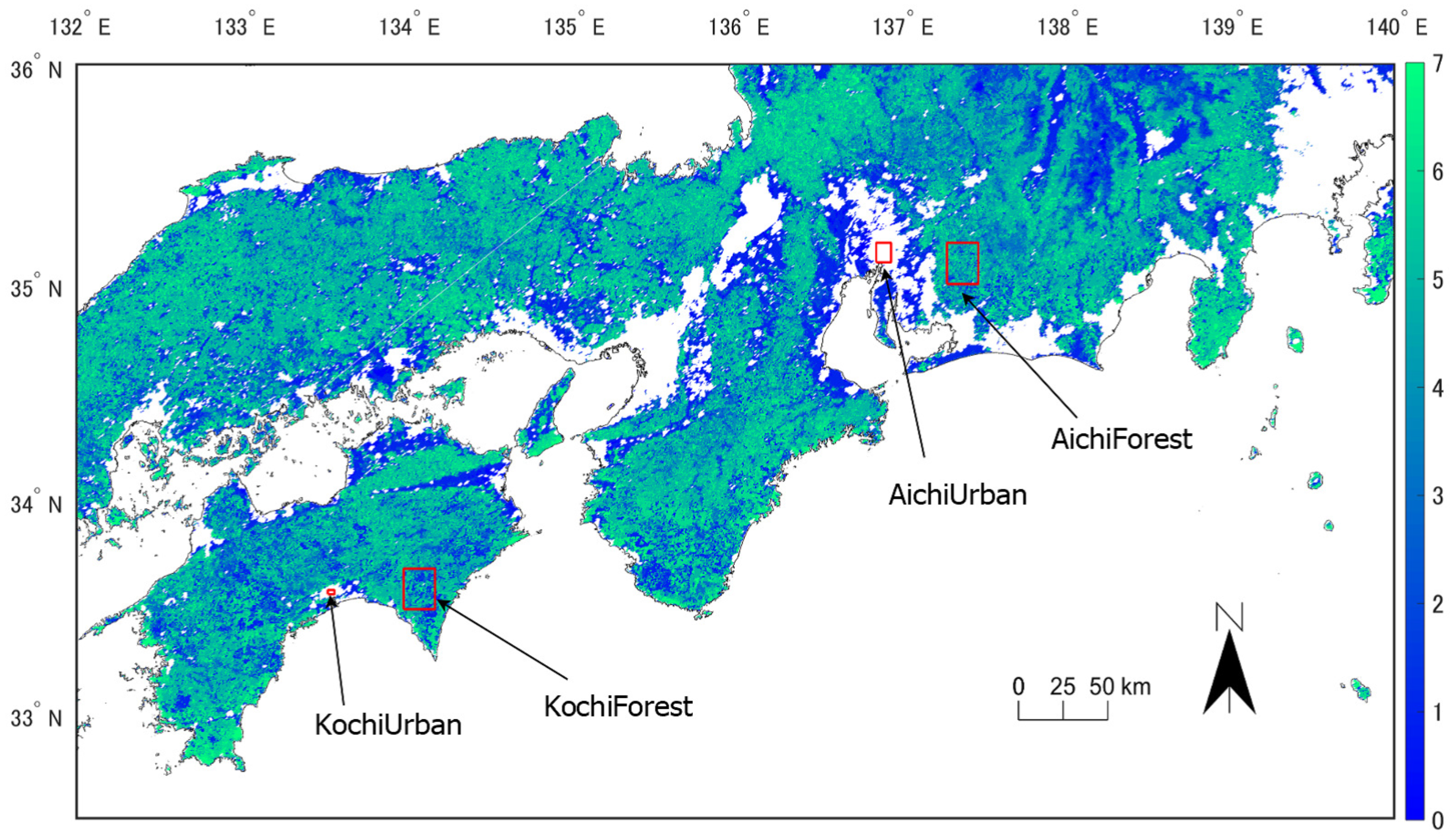
Figure 3.
Spatial distribution of the LAI in the western part of Japan, based on the MOD15A2H data collected on 17 May 2017. Four ROIs are indicted by rectangles. LAI values of the non-vegetated regions, such as the urban and ocean regions, are represented by the white background.
Figure 3.
Spatial distribution of the LAI in the western part of Japan, based on the MOD15A2H data collected on 17 May 2017. Four ROIs are indicted by rectangles. LAI values of the non-vegetated regions, such as the urban and ocean regions, are represented by the white background.
Figure 4.
Flow chart describing the algorithm used for GEO-LEO reflectance comparisons (AHI and MODIS); (a) geometric condition retrieval; and (b) preprocessing, screening, and subsequent processing for comparison.
Figure 4.
Flow chart describing the algorithm used for GEO-LEO reflectance comparisons (AHI and MODIS); (a) geometric condition retrieval; and (b) preprocessing, screening, and subsequent processing for comparison.
Figure 5.
Overview of the AHI data composite. AHI data collected over seven consecutive days were used to create a single image for each of the SZM and RAM methods (for a total of two images). The SZM and RAM images differed with respect to the data acquisition time. The central date of the AHI observation period is the same as that designated for the MODIS data.
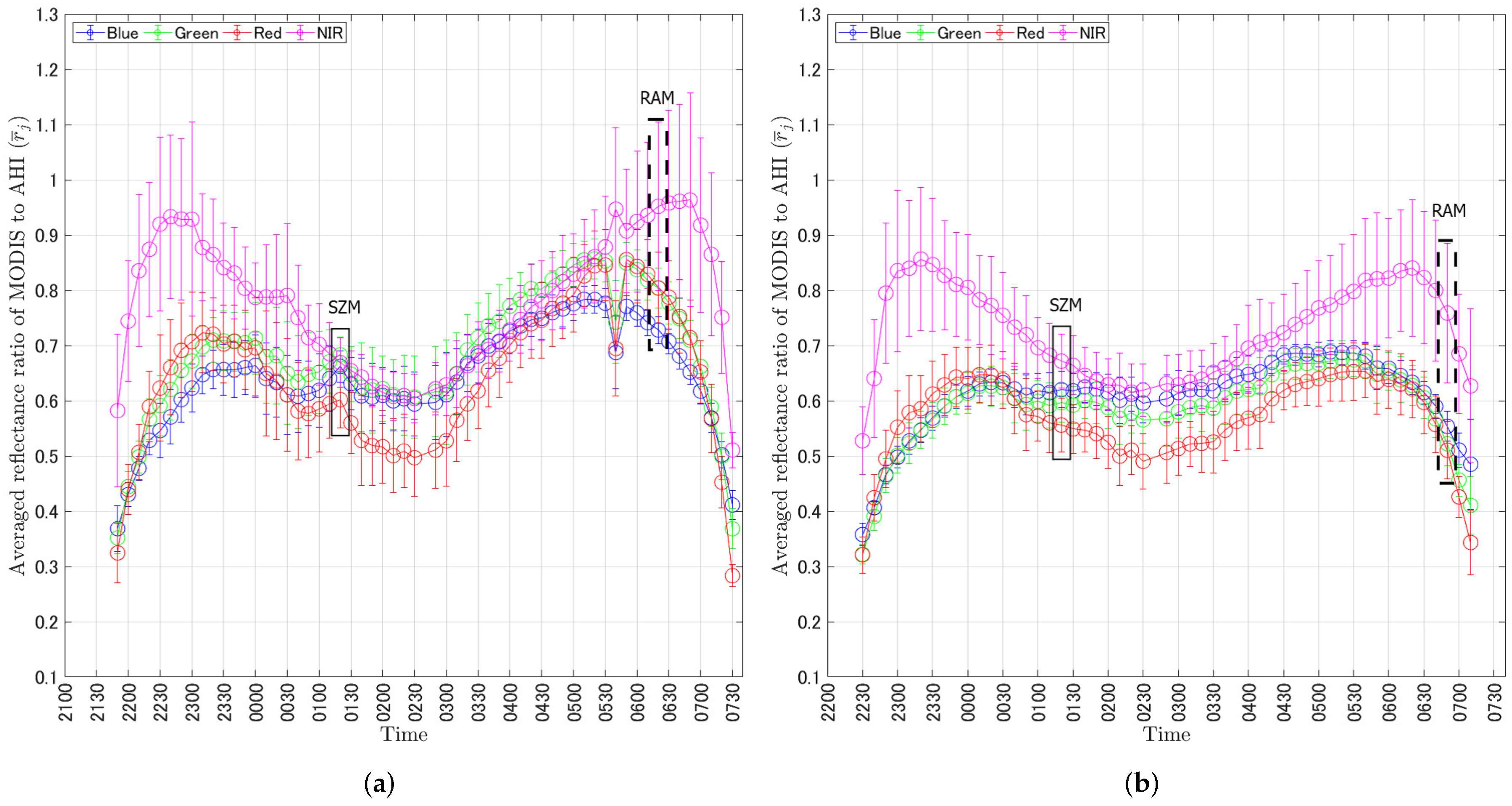
Figure 6.
Area-averaged reflectance ratios (MODIS/AHI) in the four bands, by month. The upper two plots correspond to the Kochi Forest, SZM (a) and RAM (b). The lower two plots correspond to the Aichi Forest, SZM (c) and RAM (d). The differences between the MODIS and AHI solar zenith and relative azimuth angle observations are plotted on the secondary y-axis.
Figure 7.
Area-averaged reflectance ratio (MODIS/AHI) for the urban ROIs. The upper two plots correspond to the Kochi Urban, SZM (a) and RAM (b). The lower two plots correspond to the Aichi Urban, SZM (c) and RAM (d).
Figure 7.
Area-averaged reflectance ratio (MODIS/AHI) for the urban ROIs. The upper two plots correspond to the Kochi Urban, SZM (a) and RAM (b). The lower two plots correspond to the Aichi Urban, SZM (c) and RAM (d).
Figure 8.
Integrated values of Ej = |1 − | over the four bands, obtained using the SZM and RAM methods. Differences in the MODIS and AHI relative azimuth angles and solar zenith angles are plotted on the secondary y-axis: (a) Kochi Forest; (b) Aichi Forest; (c) Kochi Urban; and (d) Aichi Urban.
Figure 8.
Integrated values of Ej = |1 − | over the four bands, obtained using the SZM and RAM methods. Differences in the MODIS and AHI relative azimuth angles and solar zenith angles are plotted on the secondary y-axis: (a) Kochi Forest; (b) Aichi Forest; (c) Kochi Urban; and (d) Aichi Urban.
Figure 9.
Same plot (
Ej) as shown in
Figure 8, but only over the red and NIR bands: (
a) Kochi Forest; (
b) Aichi Forest; (
c) Kochi Urban; and (
d) Aichi Urban.
Figure 9.
Same plot (
Ej) as shown in
Figure 8, but only over the red and NIR bands: (
a) Kochi Forest; (
b) Aichi Forest; (
c) Kochi Urban; and (
d) Aichi Urban.
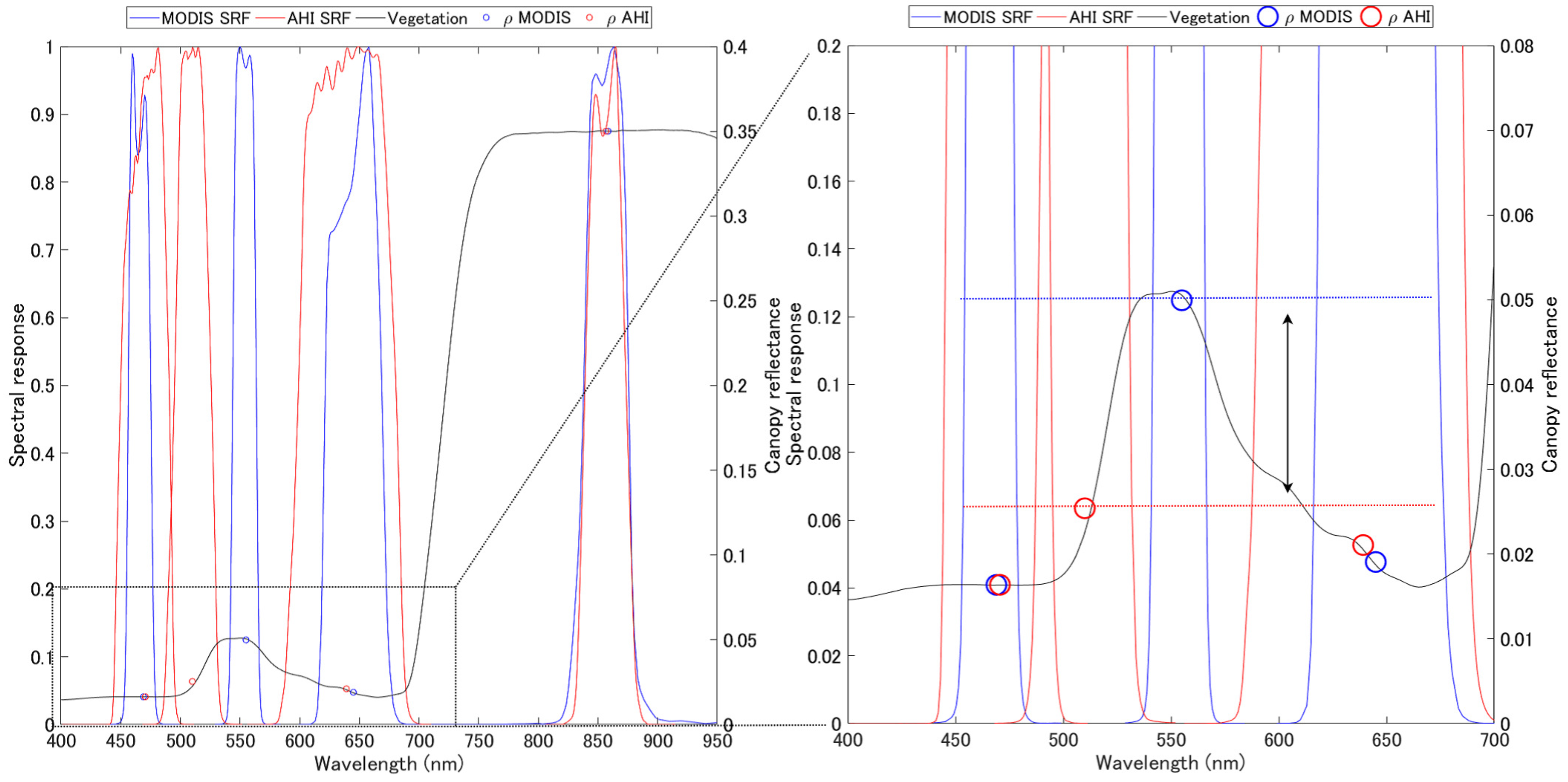
Figure 10.
SRFs for the AHI and MODIS, and spectral reflectances of the vegetation canopy simulated using PROSAIL. The values of LAI and psoil were assumed to be 2.5 and 0.0, respectively. Circles indicate the spectrally convoluted reflectances using SRFs. In the green bands, reflectance differences between AHI and MODIS were greater than in the other bands.
Figure 11.
Contour plots of the simulated MODIS to AHI reflectance ratios for (a) blue, (b) green, (c) red, and (d) NIR bands as a function of LAI and soil moisture surface effects. Ratios were close to 1.0 in the blue and NIR bands, whereas ratios were much higher than 1.0 in the green band and were smaller than 1.0 in the red band.
Figure 12.
The
values for four bands along the UTC time, from sunrise to sunset, calculated using composite data collected using the algorithm described in
Section 4.2: (
a) AichiForest on 9 November 2017; and (
b) AichiForest on 22 December 2015. Rectangles depicted by the solid and dashed lines indicate the times selected using the SZM and RAM methods, respectively.
Table 1.
Differences in the geometric and atmospheric conditions of the LEO and GEO observation pairs selected using the SZM and RAM methods. The mark “o” indicates that the GEO and LEO observation conditions are nearly identical. The numbers indicate the ranges of absolute differences in this study. The SZM method corresponds to simultaneous data acquisition; therefore, the atmospheric conditions will be identical.
| Method | Solar Zenith | View Zenith | View Azimuth | Relative Azimuth | Atmospheric Condition |
|---|
| SZM | o | o | ∼70 | 0 to 50 | o |
| RAM | 0 to 20 | o | same as SZM | o | 1.5 to 5.5 h |
Table 2.
Latitude and longitude ranges of the ROIs.
Table 2.
Latitude and longitude ranges of the ROIs.
| ROI | Range (Latitude/Longitude) |
|---|
| Forest in Kochi (KochiForest) | 33.485–33.675 N/133.985–134.175 E |
| Forest in Aichi (AichiForest) | 34.995–35.185 N/137.285–137.475 E |
| Urban in Kochi (KochiUrban) | 33.555–33.575 N/133.525–133.565 E |
| Urban in Aichi (AichiUrban) | 35.095–35.185 N/136.855–136.945 E |
Table 3.
Selected dates for the top MODIS data evaluated by the number of confident clear pixels over each ROI. Dates are represented by six characters, “YYMMDD” (Y, M, and D represent the year, month, and day, respectively). The number in parentheses is the day of the year. The third, fifth, seventh, and ninth columns show the number of pixels found to be confident clear in each ROI.
| | KochiForest | | AichiForest | | KochiUrban | | AichiUrban | |
|---|
| January | 180126 (26) | 196 | 170125 (25) | 207 | 180110 (10) | 1 | 170125 (25) | 8 |
| February | 170224 (55) | 217 | 160208 (39) | 215 | 170224 (55) | 1 | 160208 (39) | 12 |
| March | 160325 (85) | 232 | 160327 (87) | 210 | 170328 (87) | 4 | 160311 (71) | 7 |
| April | 170413 (103) | 225 | 180402 (92) | 64 | 170429 (119) | 4 | 160412 (103) | 2 |
| May | 160512 (133) | 237 | 180520 (140) | 37 | 160512 (133) | 4 | 180520 (140) | 7 |
| June | 180603 (154) | 125 | 170602 (153) | 8 | - | - | 170602 (153) | 13 |
| July | 160731 (213) | 126 | 150731 (212) | 216 | - | - | 180723 (204) | 39 |
| August | 180806 (218) | 121 | 180808 (220) | 237 | 180806 (218) | 3 | 180808 (220) | 39 |
| September | 160901 (245) | 231 | 160903 (247) | 217 | 160901 (245) | 3 | 160903 (247) | 2 |
| October | 151017 (290) | 229 | 151003 (276) | 187 | 151017 (290) | 2 | 151019 (292) | 7 |
| November | 171107 (311) | 219 | 171109 (313) | 238 | 171107 (311) | 5 | 171125 (329) | 25 |
| December | 171209 (343) | 246 | 151222 (356) | 231 | 171209 (343) | 4 | 161208 (343) | 27 |
Table 4.
UTC time and DOY for the selected AHI data in the SZM and RAM methods.
Table 4.
UTC time and DOY for the selected AHI data in the SZM and RAM methods.
| | January | February | March | April | May | June | July | August | September | October | November | December |
|---|
| DOY: KochiForest | 26 | 55 | 85 | 103 | 133 | 154 | 213 | 218 | 245 | 290 | 311 | 343 |
| time (SZM) | 0130 | 0130 | 0130 | 0130 | 0130 | 0135 | 0130 | 0135 | 0130 | 0130 | 0130 | 0130 |
| time (RAM) | 0550 | 0510 | 0420 | 0350 | 0320 | 0310 | 0320 | 0330 | 0350 | 0510 | 0550 | 0620 |
| DOY: AichiForest | 25 | 39 | 87 | 92 | 140 | 153 | 212 | 220 | 247 | 276 | 313 | 356 |
| time (SZM) | 0120 | 0120 | 0120 | 0120 | 0120 | 0120 | 0120 | 0120 | 0120 | 0120 | 0120 | 0120 |
| time (RAM) | 0620 | 0550 | 0430 | 0420 | 0310 | 0300 | 0320 | 0330 | 0400 | 0500 | 0620 | 0650 |
| DOY: KochiUrban | 10 | 55 | 87 | 119 | 133 | - | - | 218 | 245 | 290 | 311 | 343 |
| time (SZM) | 0130 | 0130 | 0130 | 0130 | 0130 | - | - | 0135 | 0130 | 0130 | 0130 | 0130 |
| time (RAM) | 0610 | 0510 | 0410 | 0330 | 0320 | - | - | 0330 | 0350 | 0510 | 0550 | 0620 |
| DOY: AichiUrban | 25 | 39 | 71 | 103 | 140 | 153 | 204 | 220 | 247 | 292 | 329 | 343 |
| time (SZM) | 0120 | 0120 | 0120 | 0120 | 0120 | 0120 | 0120 | 0120 | 0120 | 0120 | 0120 | 0120 |
| time (RAM) | 0610 | 0550 | 0450 | 0400 | 0310 | 0300 | 0320 | 0330 | 0400 | 0530 | 0640 | 0650 |
Table 5.
Thresholds ( and ) for the forest and urban ROIs.
Table 5.
Thresholds ( and ) for the forest and urban ROIs.
| | | |
|---|
| Forest | −6.5 | 0.470 |
| Urban | - | −0.037 |
Table 6.
Number of pixels paired for comparison after all screening processes had been applied. Dates are represented by six digits: “YYMMDD”.
Table 6.
Number of pixels paired for comparison after all screening processes had been applied. Dates are represented by six digits: “YYMMDD”.
| KochiF | SZM | RAM | AichiF | SZM | RAM | KochiU | SZM | RAM | AichiU | SZM | RAM |
|---|
| 180126 | 135 | 176 | 170125 | 190 | 178 | 180110 | 1 | 1 | 170125 | 8 | 8 |
| 170224 | 204 | 174 | 160208 | 186 | 194 | 170224 | 1 | 1 | 160208 | 10 | 11 |
| 160325 | 215 | 210 | 160327 | 200 | 191 | 170328 | 4 | 4 | 160311 | 7 | 7 |
| 170413 | 200 | 208 | 180402 | 39 | 46 | 170429 | 4 | 4 | 160412 | 2 | 2 |
| 160512 | 226 | 212 | 180520 | 32 | 32 | 160512 | 4 | 4 | 180520 | 7 | 7 |
| 180603 | 116 | 98 | 170602 | 8 | 8 | - | - | - | 170602 | 13 | 13 |
| 160731 | 107 | 10 | 150731 | 174 | 137 | - | - | - | 180723 | 37 | 36 |
| 180806 | 102 | 15 | 180808 | 192 | 125 | 180806 | 0 | 0 | 180808 | 38 | 36 |
| 160901 | 212 | 154 | 160903 | 188 | 197 | 160901 | 3 | 3 | 160903 | 2 | 2 |
| 151017 | 211 | 213 | 151003 | 178 | 180 | 151017 | 2 | 2 | 151019 | 6 | 7 |
| 171107 | 199 | 204 | 171109 | 119 | 225 | 171107 | 5 | 5 | 171125 | 23 | 22 |
| 171209 | 234 | 190 | 151222 | 173 | 76 | 171209 | 4 | 4 | 161208 | 25 | 17 |
Table 7.
Summary of for the two forest ROIs. Negative values indicate a better performance of the RAM method than the SZM method.
Table 7.
Summary of for the two forest ROIs. Negative values indicate a better performance of the RAM method than the SZM method.
| | KochiForest | | | | | AichiForest | | | | |
|---|
| | Doy\Band | Blue | Green | Red | NIR | Doy\Band | Blue | Green | Red | NIR |
|---|
| January | 180126 (26) | −0.291 | −0.294 | −0.339 | −0.188 | 170125 (25) | −0.091 | −0.106 | −0.153 | −0.268 |
| February | 170224 (55) | −0.111 | −0.123 | −0.137 | −0.207 | 160208 (39) | −0.073 | −0.078 | −0.103 | −0.190 |
| March | 160325 (85) | −0.044 | 0.048 | −0.091 | −0.124 | 160327 (87) | 0.023 | 0.026 | 0.007 | −0.073 |
| April | 170413 (103) | −0.072 | −0.077 | −0.051 | −0.024 | 180402 (92) | 0.093 | 0.132 | 0.040 | −0.036 |
| May | 160512 (133) | 0.115 | 0.118 | 0.048 | 0.023 | 180520 (140) | 0.011 | −0.020 | −0.077 | −0.009 |
| June | 180603 (154) | −0.016 | −0.011 | −0.133 | −0.003 | 170602 (153) | −0.023 | −0.041 | −0.103 | −0.028 |
| July | 160731 (213) | 0.060 | 0.036 | −0.022 | −0.012 | 150731 (212) | 0.007 | −0.007 | 0.040 | −0.048 |
| August | 180806 (218) | −0.053 | −0.051 | −0.108 | 0.004 | 180808 (220) | 0.074 | −0.098 | 0.114 | −0.024 |
| September | 160901 (245) | −0.033 | −0.037 | 0.051 | −0.046 | 160903 (247) | −0.042 | 0.160 | −0.121 | −0.042 |
| October | 151017 (290) | −0.169 | −0.225 | −0.263 | −0.324 | 151003 (276) | −0.128 | −0.173 | −0.186 | −0.207 |
| November | 171107 (311) | −0.204 | −0.269 | −0.357 | −0.279 | 171109 (313) | −0.066 | −0.121 | −0.202 | −0.283 |
| December | 171209 (343) | −0.059 | −0.086 | −0.140 | −0.319 | 151222 (356) | 0.066 | 0.074 | 0.046 | −0.087 |
| | Average | −0.073 | −0.081 | −0.129 | −0.125 | Average | −0.012 | −0.021 | −0.058 | −0.108 |
| | Avg. (April–September) | 0.000 | −0.004 | −0.036 | −0.010 | Avg. (April–September) | 0.020 | 0.021 | −0.018 | −0.031 |
| | Avg. (Other) | −0.146 | −0.158 | −0.221 | −0.240 | Avg. (Other) | −0.045 | −0.063 | −0.099 | −0.185 |
Table 8.
Summary of for the two urban ROIs. Negative values indicate that the RAM method performed better than the SZM method.
Table 8.
Summary of for the two urban ROIs. Negative values indicate that the RAM method performed better than the SZM method.
| | KochiUrban | | | | | AichiUrban | | | | |
|---|
| | Doy\Band | Blue | Green | Red | NIR | Doy\Band | Blue | Green | Red | NIR |
|---|
| January | 180110 (10) | −0.128 | −0.111 | −0.122 | −0.149 | 170125 (25) | −0.131 | −0.137 | −0.179 | −0.220 |
| February | 170224 (55) | −0.055 | −0.096 | −0.057 | −0.067 | 160208 (39) | −0.143 | −0.147 | −0.208 | −0.217 |
| March | 170328 (87) | −0.008 | 0.008 | 0.026 | 0.034 | 160311 (71) | −0.096 | −0.095 | −0.093 | −0.097 |
| April | 170429 (119) | 0.072 | 0.043 | −0.011 | −0.038 | 160412 (103) | 0.068 | 0.048 | 0.033 | −0.013 |
| May | 160512 (133) | 0.059 | 0.035 | −0.003 | 0.005 | 180520 (140) | −0.009 | −0.025 | −0.045 | −0.013 |
| June | - | - | - | - | - | 170602 (153) | −0.027 | −0.038 | −0.056 | −0.065 |
| July | - | - | - | - | - | 180723 (204) | −0.056 | −0.068 | −0.073 | −0.047 |
| August | - | - | - | - | - | 180808 (220) | −0.017 | −0.017 | −0.033 | −0.025 |
| September | 160901 (245) | 0.107 | 0.093 | 0.035 | 0.077 | 160903 (247) | 0.109 | 0.105 | 0.055 | −0.022 |
| October | 151017 (290) | −0.196 | −0.194 | −0.178 | −0.192 | 151019 (292) | −0.087 | −0.103 | −0.170 | −0.251 |
| November | 171107 (311) | −0.218 | −0.250 | −0.285 | −0.220 | 171125 (329) | −0.053 | −0.068 | −0.128 | −0.252 |
| December | 171209 (343) | −0.133 | −0.160 | −0.193 | −0.241 | 161208 (343) | −0.012 | −0.015 | −0.113 | −0.216 |
| | Average | −0.056 | −0.070 | −0.088 | −0.088 | Average | −0.038 | −0.047 | −0.084 | −0.120 |
| | Avg. (April–September) | 0.079 | 0.057 | 0.007 | 0.015 | Avg. (April–September) | 0.011 | 0.001 | −0.020 | −0.031 |
| | Avg. (Other) | −0.123 | −0.134 | −0.135 | −0.139 | Avg. (Other) | −0.087 | −0.094 | −0.149 | −0.209 |
Table 9.
Input parameters for the PROSAIL algorithm used in the numerical simulations. The LIDF is the leaf inclination distribution function. The parameter psoil was used to describe the moisture-induced reflectance changes in the soil surface (from wet to dry).
Table 9.
Input parameters for the PROSAIL algorithm used in the numerical simulations. The LIDF is the leaf inclination distribution function. The parameter psoil was used to describe the moisture-induced reflectance changes in the soil surface (from wet to dry).
| Canopy | |
| LAI | 0.0 (1.0 ) to 5.0 with 0.5 increment |
| LIDF (ID4LIDF) | Planophile |
| Hotspot size parameter (hspot) | 0.01 |
| Leaf structure parameter (N) | 1.5 |
| Chlorophyll content (Cab) | 40 g/cm |
| Carotenoid content (Car) | 8 g/cm |
| Brown pigment content (Cbrown) | 0.0 (unitless, fraction) |
| Geometry | |
| Equivalent water thickness (Cw) | 0.01 cm |
| Dry matter content (Cm) | 0.009 g/cm |
| psoil | 0.0–1.0 with 0.1 increment |
| Solar zenith angle (tts) | 30.0 deg |
| Viewing zenith angle (tto) | 40.0 deg |
| Relative azimuth angle (psi) | 36.0 deg |
Table 10.
Sunrise and Sunset times in the ROIs during the summer and winter solstices [
51]. Dates are represented by six digits: “YYMMDD”.
Table 10.
Sunrise and Sunset times in the ROIs during the summer and winter solstices [
51]. Dates are represented by six digits: “YYMMDD”.
| | Sunrise Time | Sunset Time |
|---|
| Aichi (Nagoya) 180621 | 180620 19:38 UTC (180621 4:38 JST) | 180621 10:10 UTC (180621 19:10 JST) |
| Aichi (Nagoya) 171222 | 171221 21:57 UTC (171222 6:57 JST) | 171222 07:45 UTC (171222 16:45 JST) |
| Kochi (Kochi) 180621 | 180620 19:56 UTC (180621 4:56 JST) | 180621 10:19 UTC (180621 19:19 JST) |
| Kochi (Kochi) 171222 | 171221 22:06 UTC (171222 7:06 JST) | 171222 08:02 UTC (171222 17:02 JST) |


