A Theoretical Analysis for Improving Aerosol-Induced CO2 Retrieval Uncertainties Over Land Based on TanSat Nadir Observations Under Clear Sky Conditions


Abstract
1. Introduction
2. Methodology
2.1. Optimal Estimation Theory
2.2. Linear Error Analysis
3. TanSat Simulations and Retrieval Assumptions
3.1. Simulation Input
3.2. The State Vector Defination
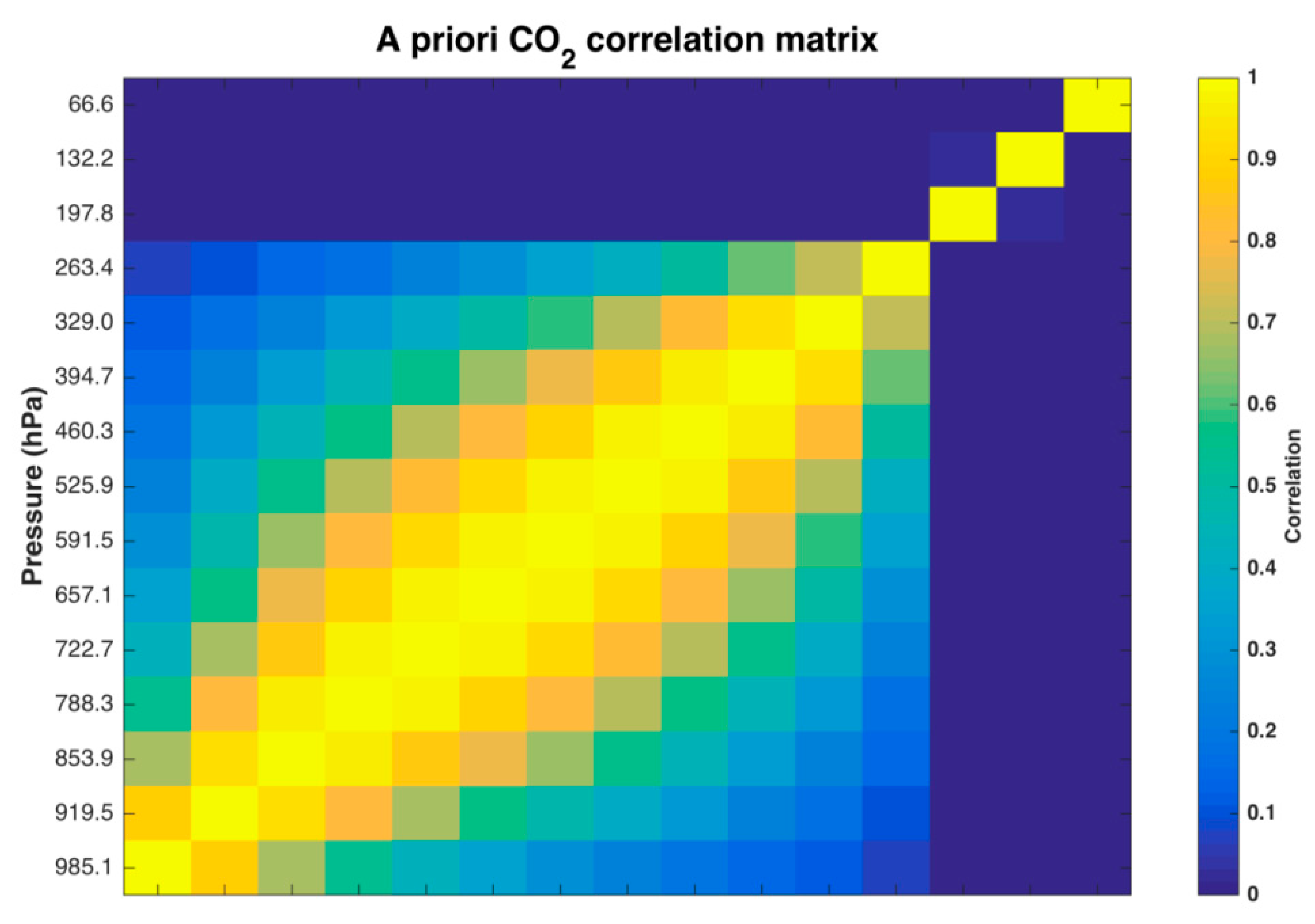
3.3. The A Priori and Measurement Error Assumptions
4. Aerosol Parameters in CO2 Retrieval
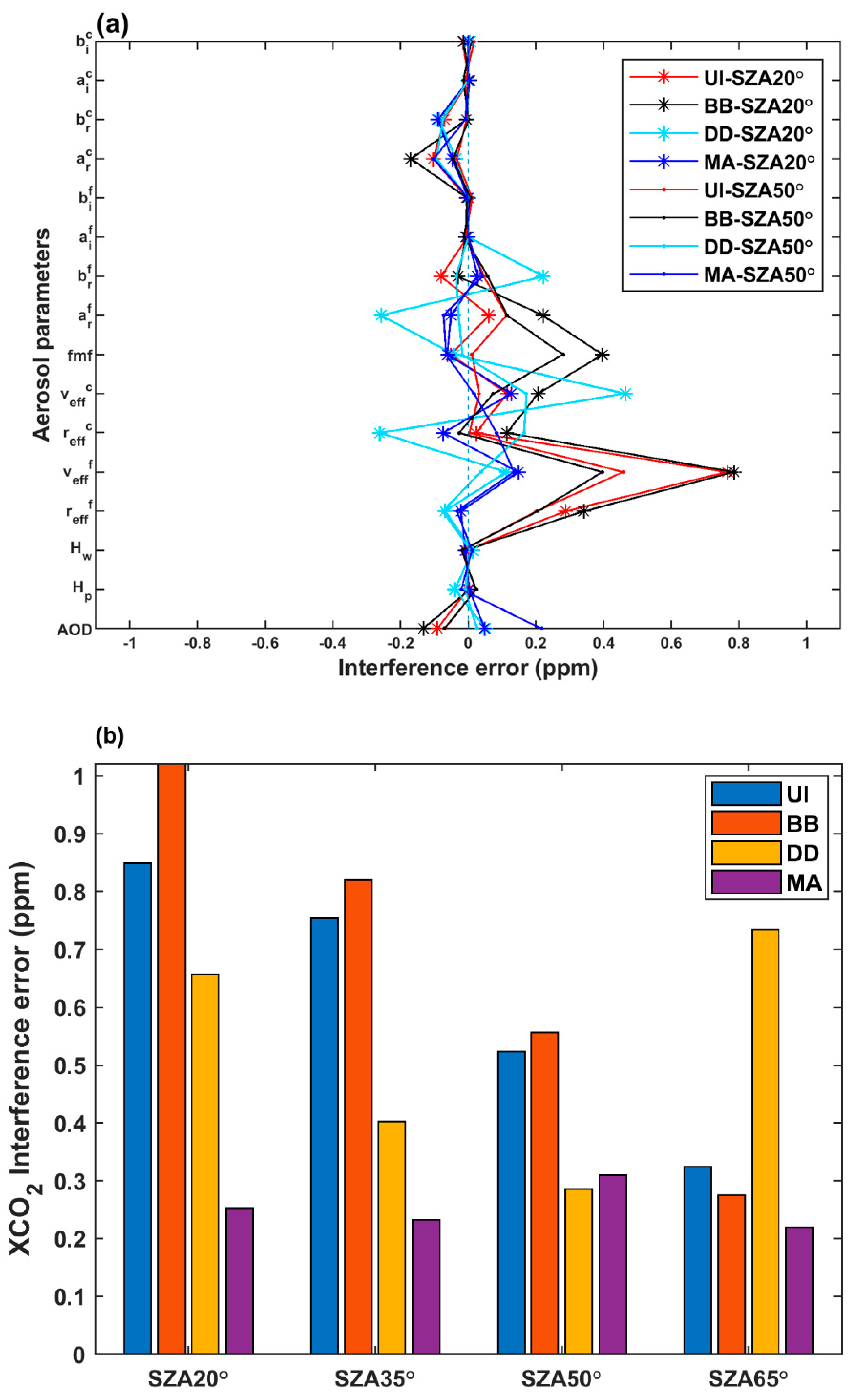
4.1. Aerosol-Induced XCO2 Retrieval Errors
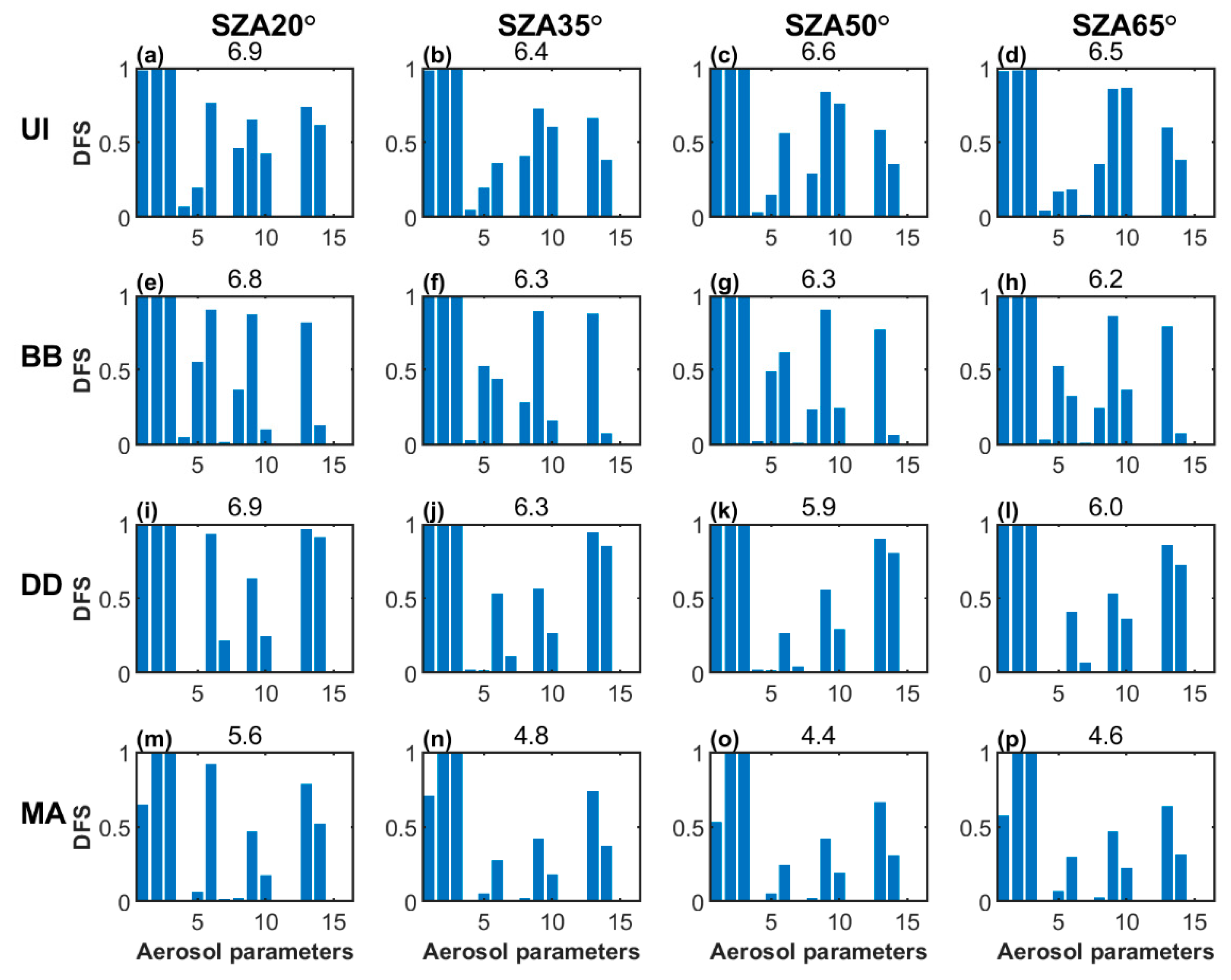
4.2. Aerosol Information
5. The Impact of Different Aerosol Models
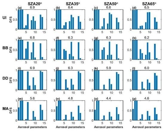
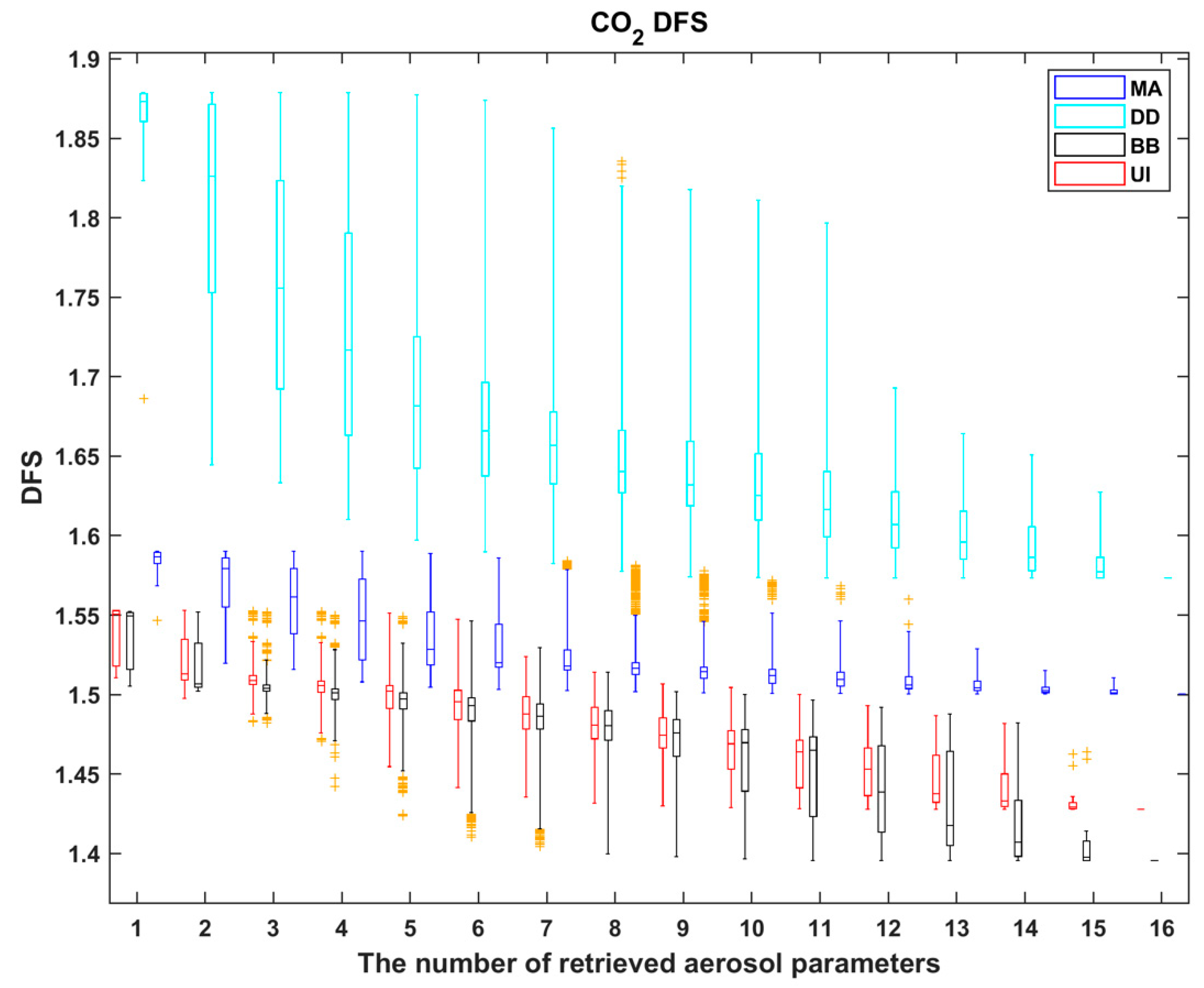
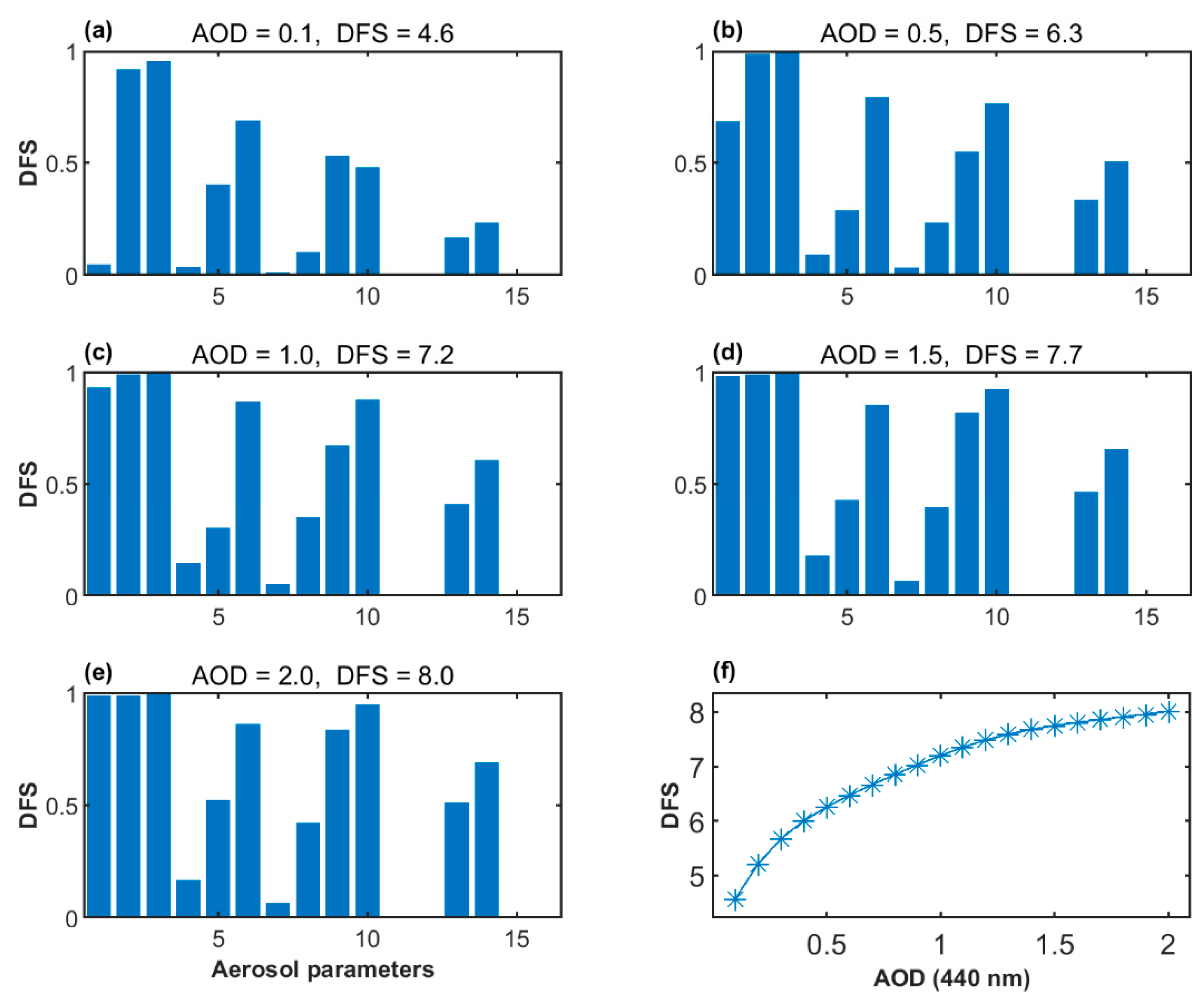
5.1. DFS of CO2
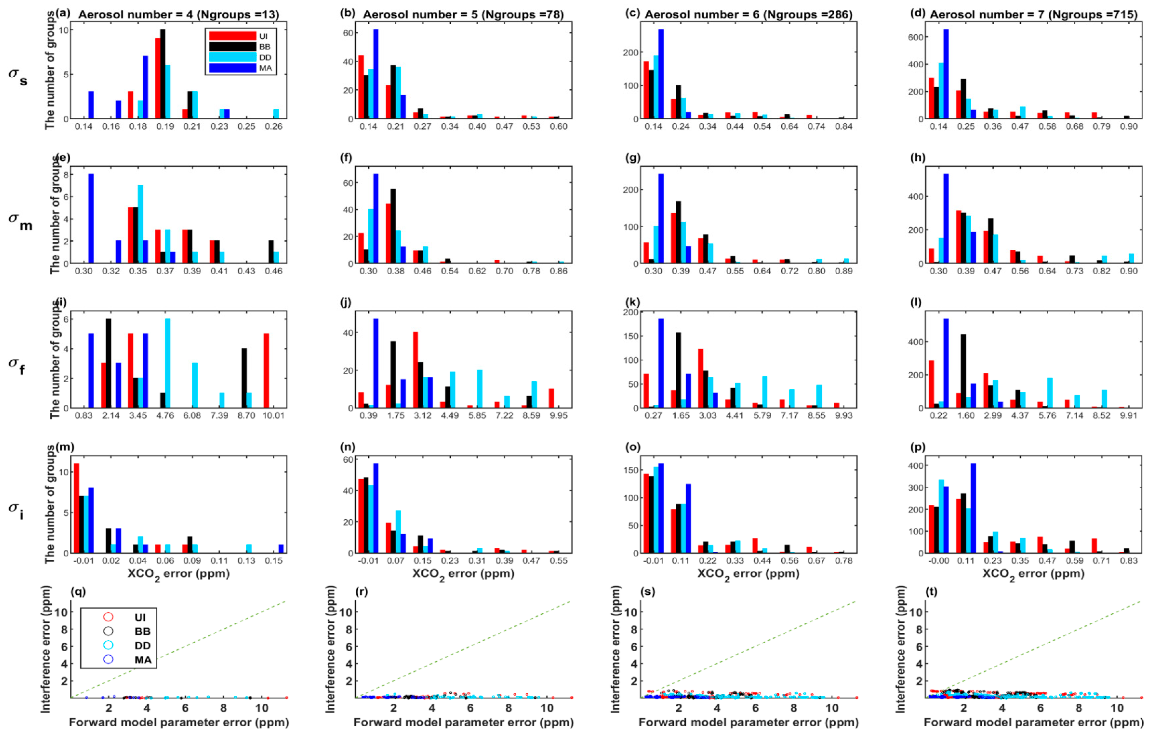
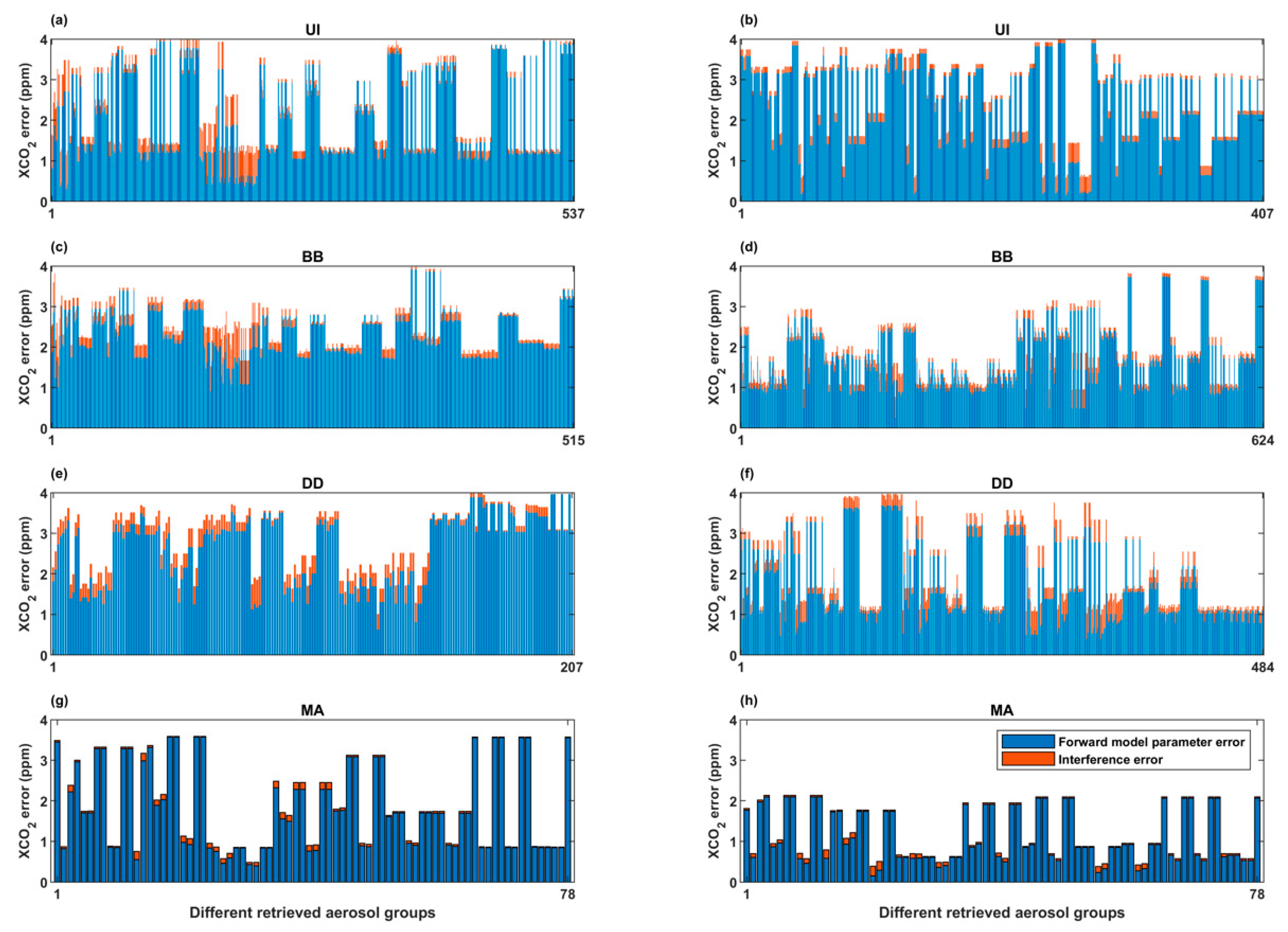
5.2. Components of XCO2 Retrieval Errors
6. Optimization of the Aerosol Model
7. Discussions
8. Conclusions
Supplementary Materials
Author Contributions
Funding
Acknowledgments
Conflicts of Interest
References
- Team, C.W.; Pachauri, R.K.; Meyer, L.A. Climate Change 2014: Synthesis Report; IPCC Press Office: Geneva, Switzerland, 2014; p. 151. [Google Scholar]
- Stocker, T.F.; Qin, D.; Plattner, G.K.; Tignor, M.; Allen, S.K.; Boschung, J.; Nauels, A.; Xia, Y.; Bex, V.; Midgley, P.M. Climate Change 2013: The Physical Science Basis. Contribution of Working Group I to the Fifth Assessment Report of the Intergovernmental Panel on Climate Change; Cambridge University Press: Cambridge, UK, 2013. [Google Scholar]
- Kuze, A.; Suto, H.; Nakajima, M.; Hamazaki, T. Thermal and near infrared sensor for carbon observation Fourier-transform spectrometer on the Greenhouse Gases Observing Satellite for greenhouse gases monitoring. Appl. Opt. 2009, 48, 6716. [Google Scholar] [CrossRef] [PubMed]
- Yokota, T.; Yoshida, Y.; Eguchi, N.; Ota, Y.; Tanaka, T.; Watanabe, H.; Maksyutov, S. Global Concentrations of CO2 and CH4 Retrieved from GOSAT: First Preliminary Results. SOLA 2009, 5, 160–163. [Google Scholar] [CrossRef]
- Nobuta, K.; Morino, I.; Yoshida, Y.; Ota, Y.; Eguchi, N.; Kikuchi, N.; Tran, H.; Yokota, T. Retrieval algorithm for CO2 and CH4 column abundances from short-wavelength infrared spectral observations by the Greenhouse gases observing satellite. Atmos. Meas. Tech. 2011, 4, 717–734. [Google Scholar]
- Maksyutov, S.; Takagi, H.; Valsala, V.K.; Saito, M.; Oda, T.; Saeki, T.; Belikov, D.A.; Saito, R.; Ito, A.; Yoshida, Y.; et al. Regional CO2 flux estimates for 2009–2010 based on GOSAT and ground-based CO2 observations. Atmos. Chem. Phys. Discuss. 2013, 13, 9351–9373. [Google Scholar] [CrossRef]
- Deng, F.; Jones, D.B.A.; O’Dell, C.W.; Nassar, R.; Parazoo, N.C. Combining gosat xco2 observations over land and ocean to improve regional CO2 flux estimates. J. Geophys. Res. Atmos. 2016, 121, 1896–1913. [Google Scholar] [CrossRef]
- Eldering, A.; O’dell, C.W.; Wennberg, P.O.; Crisp, D.; Gunson, M.R.; Viatte, C.; Avis, C.; Braverman, A.; Castano, R.; Chang, A.; et al. The Orbiting Carbon Observatory-2: first 18 months of science data products. Atmos. Meas. Tech. 2017, 10, 549–563. [Google Scholar] [CrossRef]
- Eldering, A.; Wennberg, P.O.; Crisp, D.; Schimel, D.S.; Gunson, M.R.; Chatterjee, A.; Liu, J.; Schwandner, F.M.; Sun, Y.; O’Dell, C.W.; et al. The Orbiting Carbon Observatory-2 early science investigations of regional carbon dioxide fluxes. Science 2017, 358, eaam5745. [Google Scholar] [CrossRef]
- Liu, Y.; Yang, D.; Cai, Z. A retrieval algorithm for TanSat XCO2 observation: Retrieval experiments using GOSAT data. Chin. Sci. 2013, 58, 1520–1523. [Google Scholar] [CrossRef]
- Li, Z.; Lin, C.; Li, C.; Wang, L.; Ji, Z.; Xue, H.; Wei, Y.; Gong, C.; Gao, M.; Liu, L. Prelaunch spectral calibration of a carbon dioxide spectrometer. Meas. Sci. Technol. 2017, 28, 6. [Google Scholar] [CrossRef]
- Zhang, H.; Zheng, Y.; Lin, C.; Wang, W.; Wang, Q.; Li, S. Laboratory spectral calibration of TanSat and the influence of multiplex merging of pixels. Int. J. Sens. 2017, 38, 3800–3816. [Google Scholar] [CrossRef]
- Yang, D.; Liu, Y.; Cai, Z.; Chen, X.; Yao, L.; Lu, D. First Global Carbon Dioxide Maps Produced from TanSat Measurements. Adv. Atmos. Sci. 2018, 35, 621–623. [Google Scholar] [CrossRef]
- Rayner, P.J.; O’Brien, D.M. The utility of remotely sensed CO2 concentration data in surface source inversions. Geophys. Lett. 2001, 28, 175–178. [Google Scholar] [CrossRef]
- Aben, I.; Hasekamp, O.; Hartmann, W. Uncertainties in the space-based measurements of CO2 columns due to scattering in the Earth’s atmosphere. J. Quant. Spectrosc. Radiat. Transf. 2007, 104, 450–459. [Google Scholar] [CrossRef]
- Connor, B.; Boesch, H.; McDuffie, J.; Taylor, T.; Fu, D.; Frankenberg, C.; O’dell, C.; Payne, V.; Gunson, M.; Pollock, R.; et al. Quantification of Uncertainties in OCO-2 Measurements of XCO2: Simulations and Linear Error Analysis. Atmos. Meas. Tech. Discuss. 2016, 9, 1–30. [Google Scholar] [CrossRef]
- Connor, B.J.; Boesch, H.; Toon, G.; Sen, B.; Miller, C.; Crisp, D. Orbiting Carbon Observatory: Inverse method and prospective error analysis. J. Geophys. Res. Biogeosci. 2008, 113. [Google Scholar] [CrossRef]
- O’dell, C.W.; Connor, B.; Bosch, H.; O’brien, D.; Frankenberg, C.; Castano, R.; Christi, M.; Eldering, D.; Fisher, B.; Gunson, M.; et al. The ACOS CO2 retrieval algorithm – Part 1: Description and validation against synthetic observations. Atmos. Meas. Tech. 2012, 5, 99–121. [Google Scholar] [CrossRef]
- O’dell, C.W.; Eldering, A.; Wennberg, P.O.; Crisp, D.; Gunson, M.R.; Fisher, B.; Frankenberg, C.; Kiel, M.; Lindqvist, H.; Mandrake, L.; et al. Improved retrievals of carbon dioxide from Orbiting Carbon Observatory-2 with the version 8 ACOS algorithm. Atmos. Meas. Tech. 2018, 11, 6539–6576. [Google Scholar] [CrossRef]
- Chen, X.; Wang, J.; Liu, Y.; Xu, X.; Cai, Z.; Yang, D.; Yan, C.-X.; Feng, L. Angular dependence of aerosol information content in capi/tansat observation over land: Effect of polarization and synergy with a-train satellites. Remote Sens. Environ. 2017, 196, 163–177. [Google Scholar] [CrossRef]
- Chen, X.; Yang, D.; Cai, Z.; Liu, Y.; Spurr, R.J.D. Aerosol Retrieval Sensitivity and Error Analysis for the Cloud and Aerosol Polarimetric Imager on Board TanSat: The Effect of Multi-Angle Measurement. Remote. Sens. 2017, 9, 183. [Google Scholar] [CrossRef]
- Yoshida, Y.; Kikuchi, N.; Morino, I.; Uchino, O.; Oshchepkov, S.; Bril, A.; Saeki, T.; Schutgens, N.; Toon, G.C.; Wunch, D.; et al. Improvement of the retrieval algorithm for GOSAT SWIR XCO2 and XCH4 and their validation using TCCON data. Atmos. Meas. Tech. 2013, 6, 1533–1547. [Google Scholar] [CrossRef]
- Boesch, H.; Baker, D.; Connor, B.; Crisp, D.; Miller, C. Global Characterization of CO2 Column Retrievals from Shortwave-Infrared Satellite Observations of the Orbiting Carbon Observatory-2 Mission. Remote. Sens. 2011, 3, 270–304. [Google Scholar] [CrossRef]
- Butz, A.; Hasekamp, O.P.; Frankenberg, C.; Aben, I. Retrievals of atmospheric CO_2 from simulated space-borne measurements of backscattered near-infrared sunlight: accounting for aerosol effects. Appl. Opt. 2009, 48, 3322. [Google Scholar] [CrossRef]
- Butz, A.; Guerlet, S.; Hasekamp, O.; Schepers, D.; Galli, A.; Aben, I.; Frankenberg, C.; Hartmann, J.-M.; Tran, H.; Kuze, A.; et al. Toward accurate CO2 and CH4 observations from GOSAT. Geophys. Lett. 2011, 38, 38. [Google Scholar] [CrossRef]
- Torres, O.; Bhartia, P.K.; Herman, J.R.; Gleason, J.; Ahmad, Z. Derivation of aerosol properties from satellite measurements of backscattered ultraviolet radiation: Theoretical basis. J. Geophys. Res. Biogeosci. 1998, 103, 17099–17110. [Google Scholar] [CrossRef]
- Dubovik, O.; Sinyuk, A.; Lapyonok, T.; Holben, B.N.; Mishchenko, M.; Yang, P.; Eck, T.F.; Volten, H.; Muñoz, O.; Veihelmann, B.; et al. Application of spheroid models to account for aerosol particle nonsphericity in remote sensing of desert dust. J. Geophys. Res. Biogeosci. 2006, 111, 111. [Google Scholar] [CrossRef]
- McGarragh, G.R. Combined Multispectral/hyperspectral Remote Sensing of Tropospheric Aerosols for Quantification of Their Direct Radiative Effect. Ph.D. Thesis, Colorado State University, Fort Collins, CO, USA, 2013. [Google Scholar]
- Xu, X.; Wang, J.; Yi, W.; Jing, Z.; Torres, O.; Yang, Y.; Marshak, A.; Reid, J.; Miller, S. Passive remote sensing of altitude and optical depth of dust plumes using the oxygen A and B bands: First results from EPIC/DSCOVR at Lagrange-1 point. Geophys. Res. Lett. 2017, 44, 7544–7554. [Google Scholar] [CrossRef]
- Yang, D.; Liu, Y.; Cai, Z.; Deng, J.; Wang, J.; Chen, X. An advanced carbon dioxide retrieval algorithm for satellite measurements and its application to GOSAT observations. Sci. Bull. 2015, 60, 2063–2066. [Google Scholar] [CrossRef][Green Version]
- Yang, D.; Zhang, H.; Liu, Y.; Chen, B.; Cai, Z.; Lü, D. Monitoring carbon dioxide from space: Retrieval algorithm and flux inversion based on GOSAT data and using CarbonTracker-China. Adv. Atmos. Sci. 2017, 34, 965–976. [Google Scholar] [CrossRef]
- Rodgers, C.D. Inverse Methods for Atmospheric Sounding-Theory and Practice; World Scientific Pub Co Pte Lt: Singapore, 2000. [Google Scholar]
- Xu, X.; Wang, J. Retrieval of aerosol microphysical properties from AERONET photopolarimetric measurements: 1. Information content analysis. J. Geophys. Res. Atmos. 2015, 120, 7059–7078. [Google Scholar] [CrossRef]
- Hasekamp, O.P.; Landgraf, J. Retrieval of aerosol properties over the ocean from multispectral single-viewing-angle measurements of intensity and polarization: Retrieval approach, information content, and sensitivity study. J. Geophys. Res. Biogeosci. 2005, 110, 1–16. [Google Scholar] [CrossRef]
- Holzer-Popp, T.; Schroedter-Homscheidt, M.; Breitkreuz, H.; Martynenko, D.; Klüser, L. Improvements of synergetic aerosol retrieval for envisat. Atmos. Chem. Phys. 2008, 8, 7651–7672. [Google Scholar] [CrossRef]
- Martynenko, D.; Holzer-Popp, T.; Elbern, H.; Schroedter-Homscheidt, M. Understanding the aerosol information content in multi-spectral reflectance measurements using a synergetic retrieval algorithm. Atmos. Meas. Tech. Discuss. 2010, 3, 2579–2602. [Google Scholar] [CrossRef]
- Frankenberg, C.; Hasekamp, O.; O’dell, C.; Sanghavi, S.; Butz, A.; Worden, J.; O’Dell, C. Aerosol information content analysis of multi-angle high spectral resolution measurements and its benefit for high accuracy greenhouse gas retrievals. Atmos. Meas. Tech. 2012, 5, 1809–1821. [Google Scholar] [CrossRef]
- Geddes, A.; Bosch, H. Tropospheric aerosol profile information from high-resolution oxygen A-band measurements from space. Atmos. Meas. Tech. 2015, 8, 859–874. [Google Scholar] [CrossRef]
- Wang, J.; Xu, X.; Ding, S.; Zeng, J.; Spurr, R.; Liu, X.; Chance, K.; Mishchenko, M. A numerical testbed for remote sensing of aerosols, and its demonstration for evaluating retrieval synergy from a geostationary satellite constellation of GEO-CAPE and GOES-R. J. Quant. Spectrosc. Radiat. Transf. 2014, 146, 510–528. [Google Scholar] [CrossRef]
- Spurr, R. LIDORT and VLIDORT: Linearized pseudo-spherical scalar and vector discrete ordinate radiative transfer models for use in remote sensing retrieval problems. Light Scatt. Rev. 3 2008, 229–275. [Google Scholar]
- Liu, Y.; Wang, J.; Yao, L.; Chen, X.; Cai, Z.; Yang, D.; Yin, Z.; Gu, S.; Tian, L.; Lu, N.; et al. The TanSat mission: Preliminary global observations. Sci. Bull. 2018, 63, 1200–1207. [Google Scholar] [CrossRef]
- Peters, W.; Jacobson, A.R.; Sweeney, C.; Andrews, A.E.; Conway, T.J.; Kenneth, M.; Miller, J.B.; Bruhwiler, L.M.P.; Gabrielle, P.; Hirsch, A.I. An atmospheric perspective on north american carbon dioxide exchange: Carbontracker. Proc. Natl. Acad. Sci. USA 2007, 104, 18925–18930. [Google Scholar] [CrossRef]
- Schaaf, C.B.; Gao, F.; Strahler, A.H.; Lucht, W.; Li, X.; Tsang, T.; Strugnell, N.C.; Zhang, X.; Jin, Y.; Muller, J.-P.; et al. First operational BRDF, albedo nadir reflectance products from MODIS. Remote Sens. Environ. 2002, 83, 135–148. [Google Scholar] [CrossRef]
- Schaaf, C.; Strahler, A.; Lucht, W. An algorithm for the retrieval of albedo from space using semiempirical BRDF models. IEEE Trans. Geosci. Sens. 2000, 38, 977–998. [Google Scholar]
- Von Hoyningen-Huene, W.; Freitag, M.; Burrows, J.B. Retrieval of aerosol optical thickness over land surfaces from top-of-atmosphere radiance. J. Geophys. Res. Biogeosci. 2003, 108, 4260. [Google Scholar] [CrossRef]
- Wanner, W.; Strahler, A.H.; Li, X. On the derivation of kernels for kernel-driven models of bidirectional reflectance. J. Geophys. Res. Biogeosci. 1995, 100, 21077. [Google Scholar] [CrossRef]
- Wanner, W.; Strahler, A.H.; Lewis, P.; Muller, J.-P.; Schaaf, C.L.B.; Barnsley, M.J.; Hu, B.; Muller, J.; Li, X. Global retrieval of bidirectional reflectance and albedo over land from EOS MODIS and MISR data: Theory and algorithm. J. Geophys. Res. Biogeosci. 1997, 102, 17143–17161. [Google Scholar] [CrossRef]
- Waquet, F.; Cairns, B.; Knobelspiesse, K.; Chowdhary, J.; Travis, L.D.; Schmid, B.; Mishchenko, M.I. Polarimetric remote sensing of aerosols over land. J. Geophys. Res. Biogeosci. 2009, 114, 114. [Google Scholar] [CrossRef]
- Mishchenko, M.I.; Cairns, B.; Kopp, G.; Schueler, C.F.; Fafaul, B.A.; Hansen, J.E.; Hooker, R.J.; Itchkawich, T.; Maring, H.B.; Travis, L.D. Accurate Monitoring of Terrestrial Aerosols and Total Solar Irradiance: Introducing the Glory Mission. Am. Meteorol. Soc. 2007, 88, 677–692. [Google Scholar] [CrossRef]
- Ding, S.; Wang, J.; Xu, X. Polarimetric remote sensing in oxygen A and B bands: sensitivity study and information content analysis for vertical profile of aerosols. Atmos. Meas. Tech. 2016, 9, 2077–2092. [Google Scholar] [CrossRef]
- Dubovik, O.; Holben, B.; Eck, T.F.; Smirnov, A.; Kaufman, Y.J.; King, M.D.; Tanré, D.; Slutsker, I. Variability of Absorption and Optical Properties of Key Aerosol Types Observed in Worldwide Locations. J. Atmos. Sci. 2002, 59, 590–608. [Google Scholar] [CrossRef]
- Dubovik, O.; King, M.D. A flexible inversion algorithm for retrieval of aerosol optical properties from Sun and sky radiance measurements. J. Geophys. Res. Biogeosci. 2000, 105, 20673–20696. [Google Scholar] [CrossRef]
- Hou, W.; Wang, J.; Xu, X.; Reid, J.S.; Han, D. An algorithm for hyperspectral remote sensing of aerosols: 1. Development of theoretical framework. J. Quant. Spectrosc. Radiat. Transf. 2016, 178, 400–415. [Google Scholar] [CrossRef]
- Dubovik, O.; Smirnov, A.; Holben, B.N.; King, M.D.; Kaufman, Y.J.; Eck, T.F.; Slutsker, I. Accuracy assessments of aerosol optical properties retrieved from Aerosol Robotic Network (AERONET) Sun and sky radiance measurements. J. Geophys. Res. Biogeosci. 2000, 105, 9791–9806. [Google Scholar] [CrossRef]
- Guerlet, S.; Butz, A.; Schepers, D.; Basu, S.; Hasekamp, O.P.; Kuze, A.; Yokota, T.; Blavier, J.-F.; Deutscher, N.M.; Griffith, D.W.T.; et al. Impact of aerosol and thin cirrus on retrieving and validating XCO2 from GOSAT shortwave infrared measurements. J. Geophys. Res. Atmos. 2013, 118, 4887–4905. [Google Scholar] [CrossRef]


| Instrument Characteristics | Value | ||
|---|---|---|---|
| Band name or number | O2-A | CO2 weak | CO2 strong |
| Spectral range (nm) | 758–778 | 1594–1624 | 2041–2081 |
| Center wavelength (nm) | 768 | 1610 | 2060 |
| FWHM (nm) 1 | 0.04 | 0.12 | 0.16 |
| SNR 1 | 360 | 250 | 180 |
| Spatial resolution (km) | 1 × 2 | ||
| Scan range (o) | −30~10 | ||
| Swath (km) | 20 | ||
| Center Wavelength (nm) | |||
|---|---|---|---|
| 768 | 0.8632/0.2525 2 | 0.1747/0.1650 | 0.2569/0.0226 |
| 1610 | 0.2107/0.4197 | 0.1100/0.1670 | 0.0286/0.0550 |
| 2060 | 0.1052/0.3279 | 0.0305/0.0826 | 0.0236/0.0670 |
| Aerosol Type | Urban–Industrial | Biomass Burning | Desert Dust | Marine Aerosol |
|---|---|---|---|---|
| AERONET site | Beijing_RADI (China) | Alta Floresta (Brazil) | Capo Verde (Capo Verde) | Lanai (Hawaii, USA) |
| Time and number of measurements (total) | 2012–2017 (Jun–Sep) 306 (1119) 2 | 2011–2016 (Aug–Oct) 163 (374) 2 | 2012–2017 1012 (1012) 2 | 1998–2004 1167 (1167) 2 |
| Number of measurements (chosen) 3 | 168 | 156 | 401 | 1167 |
| AOD range | 0.4 ≤ AOD440 ≤ 3.4 | 0.4 ≤ AOD440 ≤ 2.8 | 0.3 ≤ AOD1020 ≤ 1.7 | 0.007 ≤ AOD1020 ≤ 0.37 |
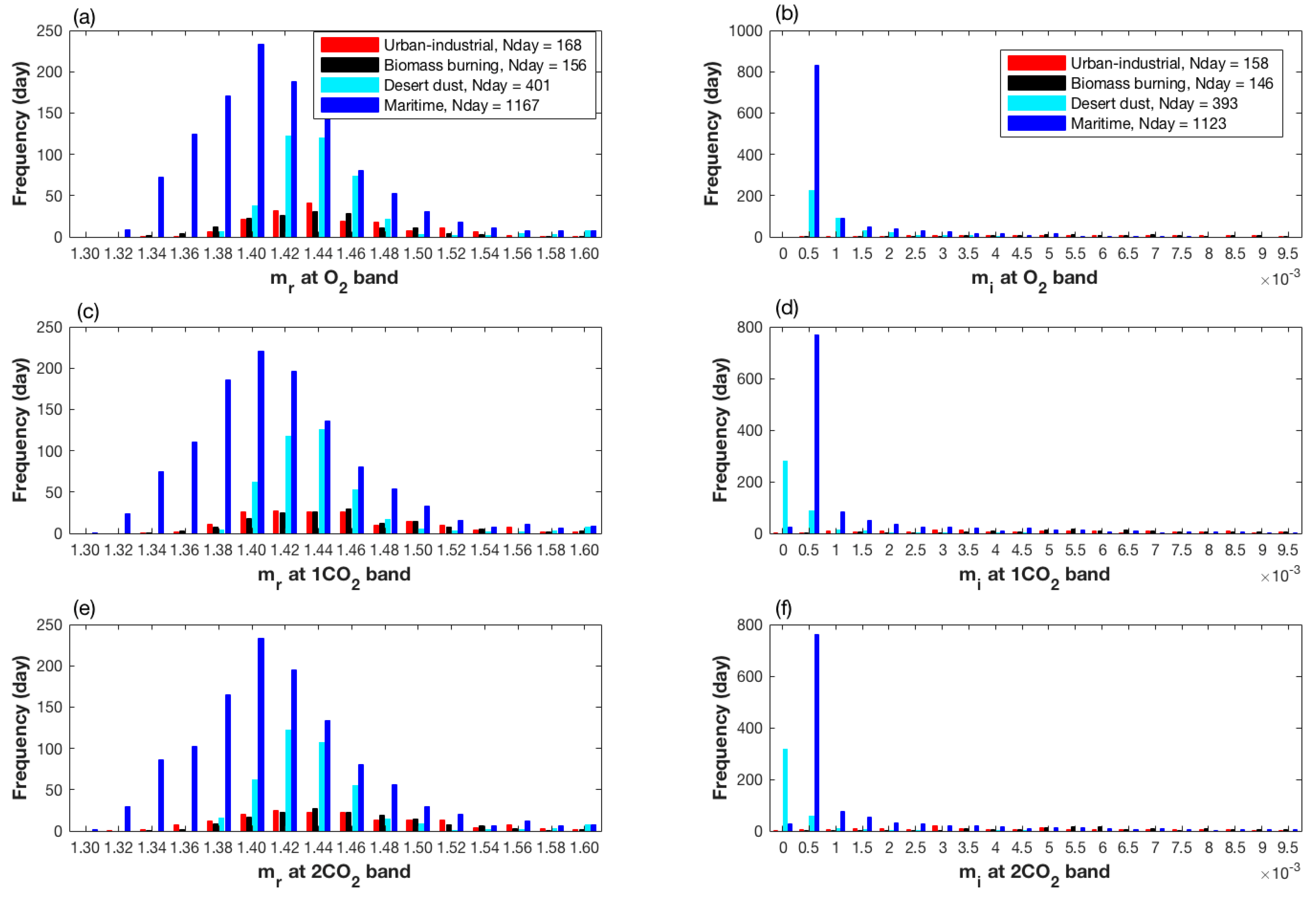
| mr 4 | 1.459 ± 0.04/1.461 ± 0.05/1.461 ± 0.06 | 1.450 ± 0.04/1.462 ± 0.05/1.466 ± 0.05 | 1.452 ± 0.04/1.448 ± 0.04/1.446 ± 0.04 | 1.42 ± 0.05 |
| mi 4 | 0.0081 ± 0.015/0.0059 ± 0.015/0.0052 ± 0.015 | 0.0078 ± 0.015/0.0069 ± 0.015/0.0066 ± 0.015 | 0.0009 ± 0.003/0.0003 ± 0.011/0.0002 ± 0.016 | 0.0005 ± 0.008 |
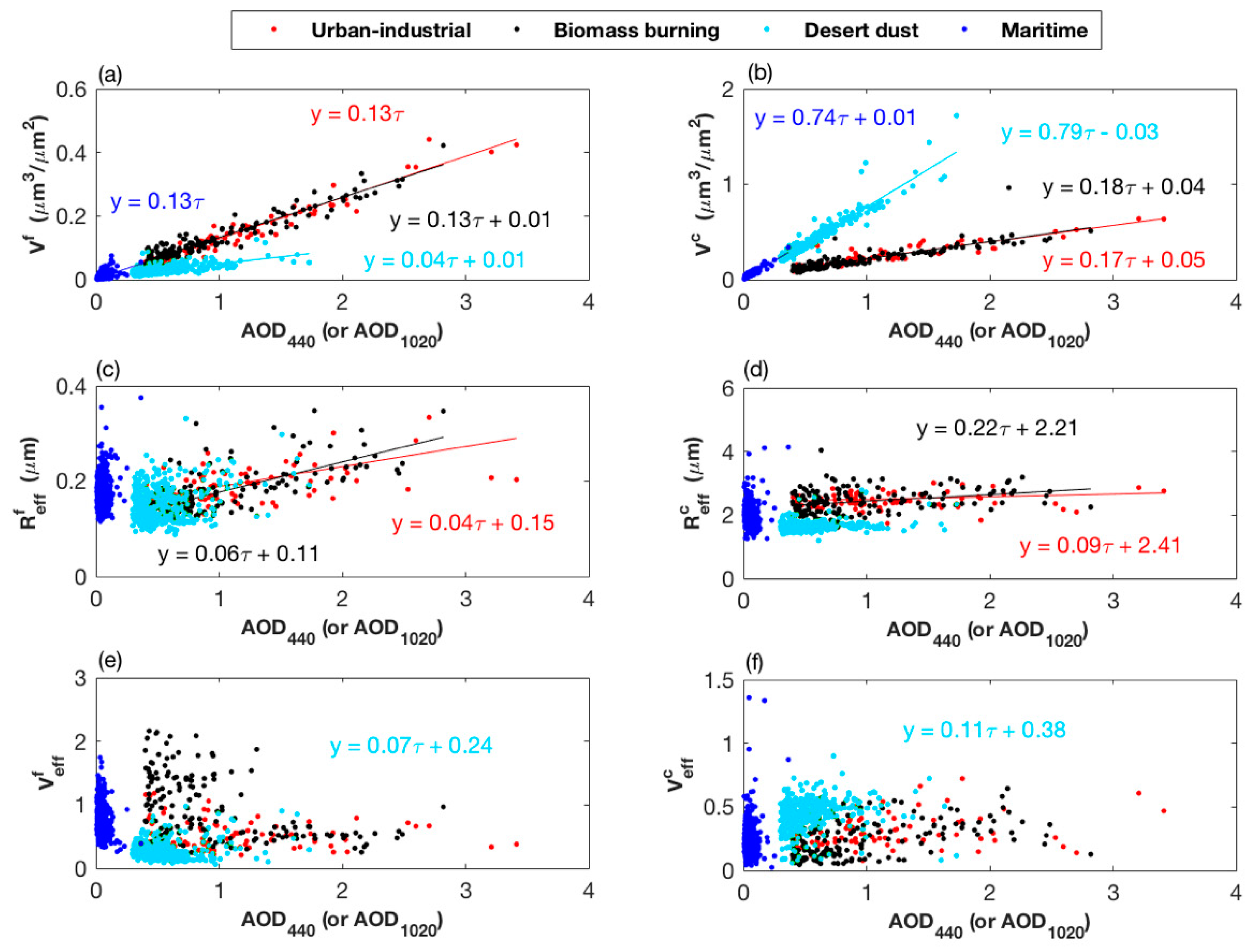
| refff (μm)/vefff | y = 0.04AOD440 + 0.15 ± 0.04/0.57 ± 0.24 | y = 0.06AOD440 + 0.11 ± 0.035/0.96 ± 0.52 | 0.15 ± 0.04/y = 0.07AOD1020 + 0.24 ± 0.14 | 0.16 ± 0.03/0.75 ± 0.19 |
| reffc (μm)/veffc | y = 0.09AOD440 + 2.41 ± 0.30/0.32 ± 0.12 | y = 0.22AOD440 + 2.21 ± 0.38/0.24 ± 0.14 | 1.64 ± 0.16/y = 0.11AOD1020 + 0.38 ± 0.12 | 1.99 ± 0.26/0.20 ± 0.10 |
| Vf (μm3/μm2) | y = 0.13AOD440 ± 0.02 | y = 0.13AOD440 + 0.01 ± 0.02 | y = 0.04AOD1020 + 0.01 ± 0.01 | y = 0.13AOD1020 ± 0.007 |
| Vc (μm3/μm2) | y = 0.17AOD440 + 0.05 ± 0.06 | y = 0.18AOD440 + 0.04 ± 0.06 | y = 0.79AOD1020 − 0.03 ± 0.055 | y = 0.74AOD1020 + 0.01 ± 0.009 |
| Parameter | Number of Parameters | a priori Uncertainty (1σ) | |
|---|---|---|---|
| CO2 (ppm) | Mixing ratio profile | 15 | (21.28, 16.7, 13.3, 9.86, 8.0, 7.09, 6.5, 6.0, 5.53, 4.79, 3.87, 2.75, 1.96, 1.84, 3.72) |
| H2O (ppm) | Scaling factor of mixing ratio profile | 1 | 50% |
| Surface pressure (hPa) | Pressure at surface layer | 1 | 1% |
| Aerosol | Aerosol optical depth (AOD) | 1 | 100% |
| The effective radius (reff) of particle size distribution (PSD) for each mode | 1 × 2 | From AERONET | |
| The effective variance (veff) of PSD for each mode | 1 × 2 | From AERONET | |
| The peak height of aerosol profile (Hp) | 1 | 100% | |
| The half width of aerosol profile (Hw) | 1 | 100% | |
| Fine mode fraction (fmf) | 1 | 100% | |
| Parameters for real part of refractive index for each mode (ar, br) 1 | 2 × 2 | From AERONET | |
| Parameters for imaginary part of refractive index for each mode (ai, bi) 1 | 2 × 2 | From AERONET | |
| Surface | BRDF coefficient of Lambertian kernel in each band | 1 × 3 | 20% |
| Aerosol Types | Group 1 | Group 2 | Group 3 | Group 4 | |
|---|---|---|---|---|---|
| Retrieved aerosol parameters 1 | UI | (AOD, Hp, Hw, vefff, reffc, arf, arc) | (AOD, Hp, Hw, reffc, arf, brf, arc) | (AOD, Hp, Hw, reffc, fmf, arf, arc) | (AOD, Hp, Hw, vefff, arf, brf, arc) |
| BB | |||||
| DD | (AOD, Hp, Hw, reffc, arf, arc, brc) | ||||
| MA | (AOD, Hp, Hw, reffc, arc) | ||||
| Total aerosol-induced XCO2 retrieval errors (ppm) | UI | 1.1986/1.3702 2 | 1.2907/0.5883 | 1.2463/1.4326 | 1.1998/0.7986 |
| BB | 1.5241/0.7762 | 2.0871/0.9462 | 1.9109/0.9569 | 1.6671/1.0424 | |
| DD | 1.6421/1.1227 | 1.5595/1.0250 | 1.6371/1.1246 | 1.0138/0.9929 | |
| MA | 0.4821/0.4836 | ||||
© 2019 by the authors. Licensee MDPI, Basel, Switzerland. This article is an open access article distributed under the terms and conditions of the Creative Commons Attribution (CC BY) license (http://creativecommons.org/licenses/by/4.0/).
Share and Cite
Chen, X.; Liu, Y.; Yang, D.; Cai, Z.; Chen, H.; Wang, M. A Theoretical Analysis for Improving Aerosol-Induced CO2 Retrieval Uncertainties Over Land Based on TanSat Nadir Observations Under Clear Sky Conditions. Remote Sens. 2019, 11, 1061. https://doi.org/10.3390/rs11091061
Chen X, Liu Y, Yang D, Cai Z, Chen H, Wang M. A Theoretical Analysis for Improving Aerosol-Induced CO2 Retrieval Uncertainties Over Land Based on TanSat Nadir Observations Under Clear Sky Conditions. Remote Sensing. 2019; 11(9):1061. https://doi.org/10.3390/rs11091061
Chicago/Turabian StyleChen, Xi, Yi Liu, Dongxu Yang, Zhaonan Cai, Hongbin Chen, and Maohua Wang. 2019. "A Theoretical Analysis for Improving Aerosol-Induced CO2 Retrieval Uncertainties Over Land Based on TanSat Nadir Observations Under Clear Sky Conditions" Remote Sensing 11, no. 9: 1061. https://doi.org/10.3390/rs11091061
APA StyleChen, X., Liu, Y., Yang, D., Cai, Z., Chen, H., & Wang, M. (2019). A Theoretical Analysis for Improving Aerosol-Induced CO2 Retrieval Uncertainties Over Land Based on TanSat Nadir Observations Under Clear Sky Conditions. Remote Sensing, 11(9), 1061. https://doi.org/10.3390/rs11091061