Article

Retrieving Phytoplankton Size Class from the Absorption Coefficient and Chlorophyll A Concentration Based on Support Vector Machine

1
State Key Laboratory of Tropical Oceanography, South China Sea Institute of Oceanology, Chinese Academy of Sciences, Guangzhou 510301, China
2
University of Chinese Academy of Sciences, Beijing 100049, China
3
College of Oceanography, Hohai University, Nanjing 210098, China
4
College of Life Sciences and Oceanography, Shenzhen University, Shenzhen 518060, China
5
South China Institute of Environmental Sciences, the Ministry of Environmental Protection of RPC, Guangzhou 510535, China
*
Author to whom correspondence should be addressed.
Remote Sens. 2019, 11(9), 1054; https://doi.org/10.3390/rs11091054
Submission received: 4 April 2019 / Revised: 1 May 2019 / Accepted: 1 May 2019 / Published: 4 May 2019
(This article belongs to the Special Issue Satellite Monitoring of Water Quality and Water Environment)

Abstract

:
The phytoplankton size class (PSC) plays an important role in biogeochemical processes in the ocean. In this study, a regional model of PSCs is proposed to retrieve vertical PSCs from the total minus water absorption coefficient (at-w(λ)) and Chlorophyll a concentration (Chla). The PSC model is developed by first reconstructing phytoplankton absorption and Chla from at-w(λ), and then extracting PSC from them using the support vector machine (SVM). In situ bio-optical data collected in the South China Sea from 2006 to 2013 were used to train the SVM. The proposed PSC model was subsequently validated using an independent PSC dataset from the Northeast South China Sea Cruise in 2015. The results indicate that the PSC model performed better than the three components model, with a value of r2 between 0.35 and 0.66, and the absolute percentage difference between 56% and 181%. On the whole, our PSC model shows a remarkable utility in terms of inferring vertical PSCs from the South China Sea.

Graphical Abstract

1. Introduction

Marine phytoplankton contribute approximately 40%–50% of the total primary production on Earth, and modulates the exchange of CO2 gas between the air and the sea [1,2,3]. Phytoplankton have different morphological (size- and shape-related) and physiological characteristics, as well as biogeochemical and ecological functions [4]. The size of phytoplankton is a good indicator of its functional roles and thus plays a fundamental role in marine ecology and biogeochemical processes. For example, the nutrient uptake and cycles, energy transfer through the marine food web, the rate of photosynthesis, deep-ocean carbon export, and gas exchange with the atmosphere are directly or indirectly related to the size of phytoplankton [5,6,7,8,9]. The phytoplankton size class (PSC) method involves partitioning the autotrophic pool into groups of different sizes, i.e., pico-plankton (<2 μm), nano-plankton (2–20 μm), and micro-plankton (>20 μm) [10]. This classification can effectively distinguish their functional types in biogeochemical processes.
Several attempts have been made to retrieve PSC from bio-optical properties. The relevant methods of retrieval can be roughly partitioned into two categories: abundance-based approaches and spectral approaches [11]. Abundance-based approaches (also known as the abundance method) simply assume that the PSC changes with a change in chlorophyll a concentration (Chla), and mainly depend on statistical relationships between in situ measurements of phytoplankton abundance and their size classes [12,13,14,15]. Spectral approaches rely on optical characteristics of phytoplankton or total particulate spectra that vary as a function of phytoplankton size, including spectral absorption-based approaches [16,17,18,19,20] and spectral backscattering-based approaches [21]. Spectral absorption-based approaches rely on the fact that pico-phytoplankton display higher Chla-specific absorption coefficients at blue wavelengths and steeper peaks with respect to larger phytoplankton. The spectral backscattering-based approaches assume that small particles have enhanced backscattering at shorter wavelengths whereas large particles display a flatter backscattering spectrum [11]. In general, both spectral and abundance-based methods have been used for PSC retrieval with varying degrees of success [11].
Several advanced techniques have recently been proposed to extract information regarding PSC and phytoplankton functional types (PFTs). For instance, multivariate statistical analysis has been successfully applied to estimate PSC and PFTs. Organelli et al. [22] retrieved PSC from in situ absorption spectra in the Mediterranean Sea based on multivariate partial least-squares regression. Wang et al. [23] used principal component analysis to capture the spectral variance of a normalized phytoplankton absorption spectrum, which was then used to derive phytoplankton size fractions. These methods were developed by discrete samples of in situ absorption spectra which cannot provide high depth resolution of PSCs. Moreover, machine learning techniques have been widely used to extract knowledge from large datasets. For example, hierarchical cluster analysis was applied to analyze ordinary and derivative spectra of the phytoplankton absorption coefficient with remote-sensing reflectance to discriminate the main pigments of phytoplankton containing information on PSC [24,25,26]. These methods focused on retrieving surface PSC from remote sensing reflectance. Further, artificial neural networks have been used to retrieve PSC and functional phytoplankton from bio-optical, spatial, temporal, and physical features [27,28]. These methods rely on Chla in combination with several ecological and physical variables and its computation is complex. A support vector machine (SVM) is a statistical method that uses a kernel function to maps training data into a new hyperspace and then constructs an optimal hyperplane fitting the training data. The major advantage of SVM lies in its complex fitting ability for non-linear data. Li et al. [29] used SVM-based recursive feature elimination to investigate the sensitivity of spectral features and remote sensing reflectance (Rrs(λ)), and applied them to develop PSC estimation models with SVM regression. Hu et al. [30] evaluated the effectiveness of many techniques for the estimation of PSC, and concluded that SVMs worked best in selecting sensitive features.
There is growing recognition that satellite maps of PSC provide useful measurements at the global scale, although these measurements are subject to the surface at hand [19,21,27,31,32]. Within the context of ecological studies and biogeochemical applications for studying the vertical distribution of algal species and primary production, such satellite surface PSC information is insufficient for ecological models and primary production models [15]. Indeed, many biogeochemical processes are depth-dependent, and the vertical distributions of PSCs are closely linked to ecosystems and biogeochemical processes [33]. Thus, high depth resolution and accurate vertical PSC distributions that go beyond surface PSC are urgently needed to provide continuous and fast retrieval of PSC for marine services.
In this paper, we investigate the retrieval of high depth resolution vertical profiles of PSC from the absorption coefficient and Chla based on SVM in the South China Sea (SCS). The regional PSC model consists of three steps. In the first step, in situ bio-optical datasets of phytoplankton absorption spectrum (aph(λ)) and Chla collected in the SCS from 2006 to 2013 were used to train the SVM. The second step was to reconstruct the aph(λ) and Chla from total minus water absorption coefficient (at-w(λ)) calculated using an absorption and attenuation meter (AC-S WET Labs Inc., Philomath, OR, USA). The third was to retrieve vertical PSCs from reconstructed aph(λ) and Chla by using the SVM. Performances were compared using three absorption parameters as inputs to the SVM to find the most useful one. Cross-validation tests that split the training and testing datasets in varying ratios were also performed to test the stability of the SVM. Once the PSC model had been built, it was validated by an independent dataset from the Northeast South China Sea (NESCS) Cruise, and was applied to obtain the vertical distribution of PSCs in bins 1 m in size. The accuracy of reconstructed aph(λ) were validated using a dataset from the West South China Sea (WSCS). The accuracy of our PSC model was compared with a regionally tuned version of the three-component model by Brewin et al. [12]. This study provides a method to discriminate vertical PSCs in the SCS.

2. Materials and Methods
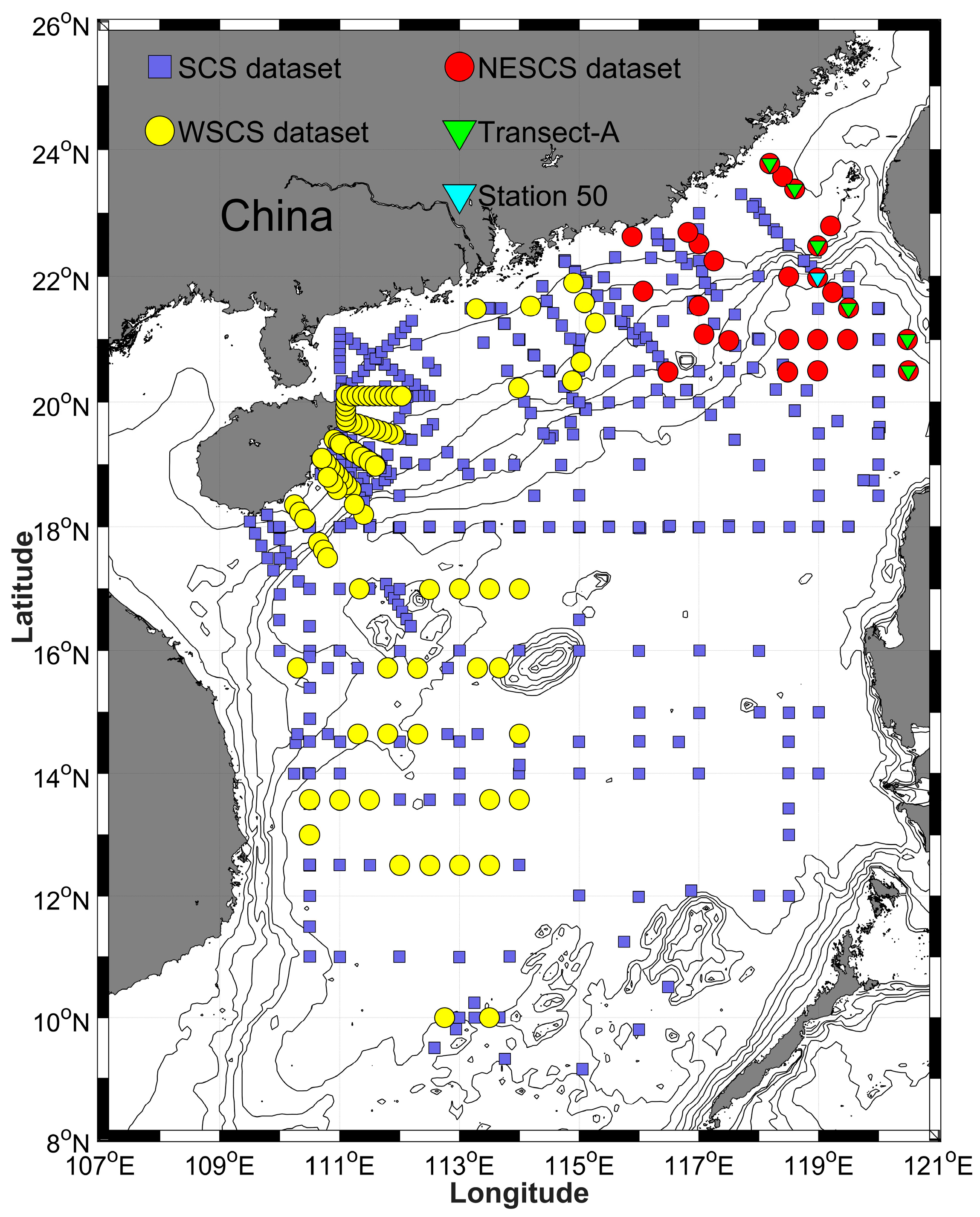
2.1. Study Area

The SCS is the largest marginal sea of the western Pacific Ocean, covering about 3.5 million square kilometers. Many complex dynamic processes occur in the SCS, including the monsoon, circulation, mesoscale eddies, and upwelling. These dynamic processes and river inputs have a significant influence on the physical, biological, and biogeochemical characteristics of the SCS [34]. A large bio-optical dataset that covered most areas of SCS from 2006 to 2013 was compiled to train the SVM in this study. The NESCS Cruise dataset, collected from the northeast of the SCS, was used as an independent dataset to validate the PSC model. The WSCS dataset collected from the west of the SCS, was used to validate the accuracy of reconstructed aph(λ). The locations of the stations used in our study are given in Figure 1.
The SCS cruise dataset from 2006 to 2013 contained 417 sets of match-ups of Chla and aph(λ) collected by the high-performance liquid chromatography (HPLC) and a UV-visible spectrophotometer (Shimadzu UV-2550, Kyoto, Japan), respectively, where a standard deviation larger than three was excluded. The NESCS dataset contained 52 sets of match-ups of at-w(λ), and in situ PSC was used to validate the independent model. The WSCS dataset contained 114 match-ups of at-w(λ) and quantitative filter-pad technique (QFT)-measured aph(λ). Lack of the match-ups of aph(λ) and at-w(λ) in NESCS, the dataset collected in the SCS but from other cruise in 2013 and 2017 (termed as WSCS) was used instead to validate the accuracy of reconstructed aph(λ) from at-w(λ) in the PSC model. The WSCS dataset contains both offshore and nearshore samples, which can provide an overall validation of aph(λ) in the SCS. Details of the datasets are shown in Table 1.

2.2. Sampling and Optical Measurements

Water samples of the phytoplankton pigment and absorption were collected using Niskin bottles at discrete layers within the photic zone. Phytoplankton absorption (aph(λ)): A suitable volume of seawater (0.5–4 L), depending on the quantity of particles, was filtered onto a 25 mm, 0.7 μm Whatman GF/F glass fiber filter under low vacuum. The filters were placed into a dark liquid nitrogen container immediately before laboratory analysis. In the laboratory, absorption spectra of the particles (ap(λ)) were measured using the QFT [35,36] with a dual-beam UV–visible spectrophotometer at a resolution of 1 nm between 350 nm and 750 nm. To obtain non-algal absorption spectra (aNAP(λ)), the filters were first extracted with methanol for 90–180 min to eliminate the phytoplankton pigment [37], and the filters were measured again using a spectrophotometer to obtain the non-algal absorption spectra. All absorption spectra were adjusted by subtracting the absorption readings at 750 nm to correct the scattering signal [38,39,40]. The amplification in path length was corrected using work by Roesler [41]. Finally, aph(λ) was calculated by estimating the difference between aP(λ) and aNAP(λ):
a p h ( λ ) = a P ( λ ) a N A P ( λ )
Phytoplankton pigments: The pigments were analyzed using an HPLC system equipped with a C8 column developed in Vidussi et al. [42]. The water samples were filtered through 25-mm Whatman GF/F filters. After sonication, they were extracted in 3 mL of HPLC-grade methanol for at least 1 day, and were refrigerated (4 °C) until analysis. Prior to injection, 500 μL of extract was mixed with 250 μL of 1 M of ammonium acetate. The extract then was injected through a 200 μL loop into the HPLC system.
Total minus water absorptions (at-w(λ)): at-w(λ) were measured by AC-S (WET Labs Inc.) over 82 wavelengths between 401.6 and 744.1 nm, and with a path length of 25 cm. Calibrations using pure water were conducted to correct the drift of the AC-S instrument and eliminate the absorption of pure water from the measured spectra. The effects of temperature and salinity on absorption were corrected using the recorded temperature and salinity during measurement [43]. The incomplete recovery of scattered light in the AC-S absorption tube was corrected by subtracting the signal at a longer wavelength (around 716 nm) from values at all other wavelengths [44].

2.3. Phytoplankton Pigment-Based Size Classes

In this study, we used the diagnostic pigment (DP) approach proposed by Uitz et al. [15], based on work by Claustre [45] and Vidussi et al. [42], to estimate the size class chlorophyll concentrations as in situ measurement of PSCs (i.e., micro-phytoplankton (Cm), nano-phytoplankton (Cn), and pico-phytoplankton (Cp)). Seven major pigments were selected from in situ HPLC pigment data as representative of distinct phytoplankton groups: fucoxanthin (Fuco), peridinin (Perid), 19’-hexanoyloxyfucoxanthin (Hex), 19’-butanoyloxyfucoxanthin (But), alloxanthin (Allo), total chlorophyll-b (chlorophyll-b + divinyl chlorophyll-b; TChlb), and zeaxanthin (Zea). The chlorophyll-a concentration can be reconstructed from the sum of concentrations of all diagnostic pigments:
DP = 1.41 [ Fuco ] + 1.41 [ Perid ] + 1.27 [ Hex Fuco ]   + 0.35 [ But Fuco ] + 0.60 [ Allo ] + 1.01 [ TChlb ] + 0.86 [ Zea ]
where D P represents the sum of concentrations of all diagnostic pigments.
The fractions of chlorophyll a concentration associated with each of the three phytoplankton classes (i.e., micro-phytoplankton (fm), nano-phytoplankton (fn), and pico-phytoplankton (fp)) were derived from the following equations by Uitz et al. [15]:
f m = ( 1.41 [ Fuco ] + 1.41 [ Perid ] ) /   D P W  
f n = ( 1.27 [ Hex Fuco ] + 0.35 [ But Fuco ] + 0.60 [ Allo ] ) /   D P W  
f p = ( 1.01 [ TChlb ] + 0.86 [ Zea ] ) /   D P W  
The fractions of each size class can then be applied to in situ Chla to derive the size class chlorophyll concentrations as follows:
Cm = f m × [ Chla ]
Cn = f n × [ Chla ]
Cp = f p × [ Chla ]

2.4. Reconstruction of aph and Chla from at-w

In this study, in situ measurement of aph(λ) and Chla were first used to develop SVM. We attempted to reconstruct aph(λ) and Chla from at-w(λ) because of its high depth resolution, and thus provided a regional PSC model just using high depth resolution of at-w(λ) as the input. Chla were first reconstructed from at-w(λ) using the absorption line height method (called the aLH method) [46]. Then, two methods were applied to decompose aph(λ) from at-w(λ). One was used to first derive Chla from at-w(λ) using the aLH method [46], and aph(λ) was then calculated from Chla using a power function [47]. To simplify the discussion, this method is called the Bricaud95 method, and consists of two steps. The second method is the stacked constraints model (called the SCM method here) proposed by Zheng et al. [48,49].
The aLH method was used to derive vertical distributions of Chla from at-w(λ) in this study. The aph(λ) or ap(λ) in the red waveband is chiefly associated with Chla for the reason that the pigment packaging in the red waveband is much less than the blue waveband [46]. As absorption by yellow matter (aCDOM(λ)) in the long waveband has less influence on at-w(λ), the aLH method was applied to aph(λ) or ap(λ) measured with QFT or with AC-S after removing the dissolved fraction as well as the at-w(λ) measured with AC-S [46]. The absorption line height at 676 nm (aLH(676)) was calculated using at-w(676), at-w(650), and at-w(715) as follows [50]:
a L H ( 676 ) = [ a t w ( 676 ) 39 / 65 a t w ( 650 ) 26 / 65 a t w ( 715 ) ]
The relationship between aLH(676) and Chla has been investigated [46,51]. The constants in this power function can be derived by regressing against aLH(676) and in situ measurements of Chla from the NESCS dataset:
RChla LH = A × a L H ( 676 ) B
where RChlaLH is the chlorophyll concentration derived by the aLH method. The values of A and B in this paper were fitted by the NESCS dataset, and were 108.07 and 1.084, respectively.
Then, aph (λ) can be calculated using a power function when RChlaLH is derived, and describes the relationship whereby aph (λ) is noticeably decreasing with increasing Chla (called the Bricaud95 method) [47]. The constants in this power function were derived by fitting against in-situ measurements of Chla and aph(λ) of the SCS dataset:
a p h ( λ ) = C ( λ ) × RChla LH D ( λ )
where aph(λ) is the phytoplankton absorption spectrum derived using the aLH method, and C(λ) and D(λ) are positive, wavelength-dependent parameters.
Unlike the Bricaud95 method derived aph(λ) from Chla, the SCM method partitions at-w(λ) directly into adg(λ) and aph(λ) with no stringent assumptions about the slope S of adg(λ) and the shape of the aph(λ). This method first finds a very wide range of speculative solutions for adg(λ) and aph(λ) and then utilizes several inequality constraints to identify a relatively narrow range of feasible solutions [48]. In this paper, we used the default SCM method and codes were shared by Zheng et al. [48,49].

2.5. Development of Vertical PSC Model

The vertical PSC model consists of two steps. The first is to reconstruct aph(λ) and Chla from at-w(λ), and the second is to use the aph(λ) and RChlaLH as inputs to the SVM to extract the PSCs.
The SVM is a statistical method that can be used to find the optimal classification boundary for binary classification problems. It uses a kernel function to solve complex classification problems with relatively low computational requirements. In this study, the SVM was used to extract information about PSCs from aph(λ) and Chla. The SCS dataset contained large amounts historical measurements of aph(λ) and Chla that were used to train the SVM. The data were mapped to the high-dimensional space by the kernel function, and the classification of the training data was achieved through structural risk minimization theory. The SVM optimization model was divided into a classification and a regression model. The optimization problem of the regression model can be expressed using the following formula:
min ω , b , ξ , ξ * 1 2 ω T ω + C i = 1 N ξ i + C i = 1 N ξ i *
Subject   to :   ω T Φ ( x i ) + b z i ε + ξ i
z i ω T Φ ( x i ) b ε + ξ i *
ξ i , ξ i * 0 , i = 1 , , N
where x i are training samples and z i are indicator vector. Φ ( x i ) maps x i into a higher-dimensional space and ω is a vector in the feature space. ξ i and ξ i * are slack variables. b is a constant and C > 0 is the regularization parameters. The SVM was implemented in MATLAB R2017b using a package in LIBSVM (https://www.csie.ntu.edu.tw/~cjlin/libsvm/).
The main steps used to develop and apply the PSC model were as follows: (1) Seek the best optical input parameters as inputs to the SVM for its development. (2) Split the SCS dataset into training and testing datasets, and test the sensitivities of the splitting ratio and random selection. (3) Use in situ measurement of aph(λ) and Chla of SCS dataset to train and develop the SVM model. (4) Reconstruct Chla from the at-w(λ) derived from AC-S using the aLH method. (5) Reconstruct aph(λ) by the Bricaud95 method, and the SCM method. (6) The regional PSC model was developed by coupling the derived aph(λ) with RChlaLH as inputs to the SVM to extract PSC information (called SVM-Bricaud95 and SVM-SCM, respectively). (7) The PSC model was validated using in situ measurements of PSCs, and was applied to profile data of AC-S from the NESCS datasets. (8) The performance of the PSC model was compared with that of the regionally tuned three-component model proposed by Brewin et al. [12]. The procedure of the development of the PSC model is summarized in a flowchart in Figure 2.

2.6. Assessments

Model skill was assessed using the coefficient of determination (r2), Pearson’s correlation coefficient (r), the absolute percentage difference (APD), and relative percentage difference (RPD), root mean-squared error (RMS). These errors are defined as follows:
RMS = 1 N n = 1 N ( y n x n ) 2
RPD = 1 N n = 1 N y n x n x n × 100 %
APD = 1 N n = 1 N | y n x n | x n × 100 %
where yn represents the retrieved value of the model, xn represents in situ values, N is the number of observations, y ¯ is the mean of the model, and x ¯ is the mean of the in situ observations.

3. Results

3.1. Distribution of PSCs

The respective contributions of pico-, nano-, and micro-phytoplankton to total biomass (i.e., fm, fn, and fp) for each sample of the SCS and NESCS datasets are displayed using a ternary plot (Figure 3).
Note that the SCS dataset contained both oligotrophic and eutrophic water samples that spanned various oceanic water types. A large number of samples of the SCS dataset were close to oligotrophic waters as they contained higher fp (60% to 95%), while few samples from the Pearl River plume and waters near the shore were eutrophic, where micro-phytoplankton dominated (fm > 80%). Numerous samples of the SCS dataset showed low amounts of nano-phytoplankton (fn < 40% for most samples). Samples from the NESCS dataset were characterized by low contributions from micro-phytoplankton (fm < 40%), and mostly showed oligotrophic water. Compared with the distributions of the SCS dataset, the NESCS dataset was generally within the regulation of the SCS dataset, and had no outlier samples beyond the general range of the SCS dataset.

3.2. Selection of Input Parameters

To train the SVM, the first step is to select the optimal input parameters. The performance of the SVM was tested using different absorption parameters as inputs. The three types of inputs chosen in the model were: (1) aph(λ) and Chla, denoted as SVM-Type1; (2) aph(λ) normalized aph(443) and Chla, denoted as SVM-Type2; and (3) aph(λ) normalized a p h ¯ and Chla, with the mean phytoplankton absorption spectrum a p h ¯   between 400 and 700 nm, denoted as SVM-Type3. In this section, the optical input was confirmed by comparing the performance of the training and test datasets. The ratio of training and test datasets was initially set at 80% and 20%, respectively.
Figure 4 illustrates the ratio of PSCs derived from the PSC model against in situ PSC, and Table 2 shows the statistics of the three different inputs derived for the PSCs. In the SCS training dataset, the median values of the ratio from the three SVM-Type were roughly around 1, while in the test dataset, relatively large deviations for Cp retrieval, especially from SVM-Type3, were noted. In addition, a significant decline in the performance of SVM-Type1 was noted between the training and test datasets, with a drop in r2 from (0.95, 0.64, 0.88) to (0.43, 0.66, 0.37) and an increase in APD from (32.20%, 25.64%, 15.15%) to (63.08%, 64.85%, 27.73%), for Cm, Cn, and Cp, respectively. Compared to SVM-Type1, SVM-Type2 and SVM-Type3 provided more stable r2 between the training and test datasets. Compared with SVM-Type3, SVM-Type2 performed better as indicated by its lower APD. Based on the statistics between the training and test datasets mentioned above, the SVM-Type2 model exhibited relatively stable performance in training and testing. Thus SVM-Type2 was selected and is discussed later.

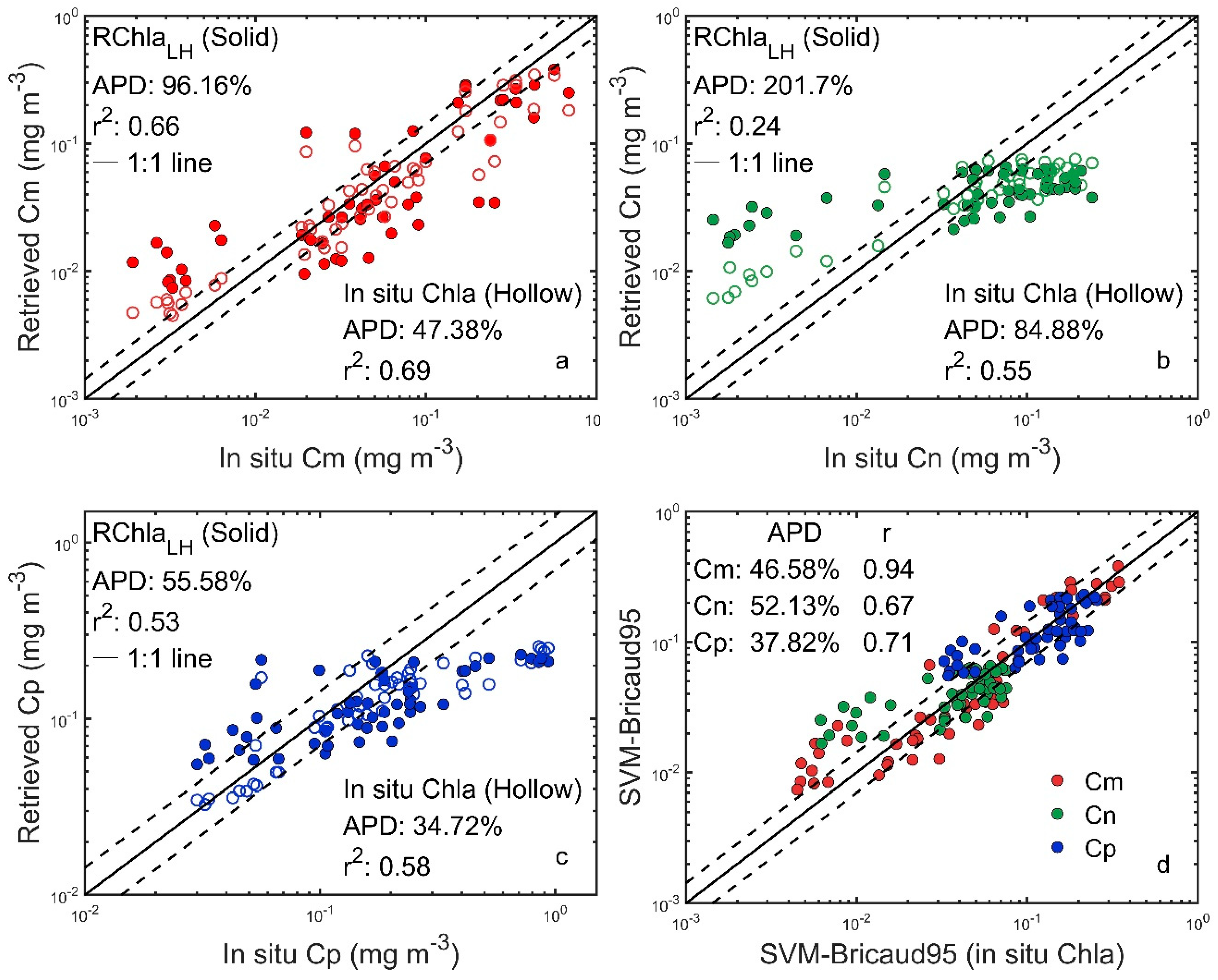
3.3. Cross-Validation Tests

After selecting the optimal input, the SCS dataset was split into training (datasets only used for SVM training) and test datasets (not involved in SVM training). In this sub-section, we assess the influence of the PSC model on the random selection of the training and test datasets for the following reasons: First, the skills of the model are influenced by the ratio of the training dataset to the testing dataset. In general, a relatively large training dataset provides more data for SVM training and yields more robust results. Second, the division of the training and test datasets should maintain the consistency of data distribution as far as possible to avoid the impact of additional deviations introduced by data divisions.
In this section, the ratio of each part is described by n (percentage of training dataset) and p (percentage of test dataset). The training dataset varied from five percent of the total dataset used for training (n = 5%) and the rest for testing (p = 95%), to 95% of the total dataset used for training (n = 95%) and five percent for testing (p = 5%), in steps of 5%. A loop program (20 times) was executed to assess each possible combination of proportions. Each possible combination of proportions also had corresponding descriptive statistics, for instance APD and r2. r2 and APD for each n are averaged over all the combinations used.
Figure 5a,b shows the variation in the statistical parameters of APD and r2 between the derived PSCs and measurements for the test datasets when the ratio of the training dataset increased from 5% to 95%. As Figure 5a shows, the APD of derived PSCs varied significantly when the ratio was less than 30%. This indicates that the SVM required a relatively large amount of data for the purposes of training. On the contrary, when the ratio was between 60% and 90%, the three derived PSC parameters (i.e., Cm, Cn, and Cp) had relatively steady APDs. The r2 values of the derived PSCs also showed a smaller variation in a similar range (≈70%–90%) of the ratio, as shown in Figure 5b. Thus, an interval between 70% and 80% was acceptable. In this study, a ratio of 80% for the training dataset (corresponding to 20% for the test dataset) was used to train the SVM.
To examine the dependence of the performance of the SVM on the training dataset, especially to avoid the effect of specific data in the training dataset on performance, we randomly picked 80% of the SCS dataset 100 times using the randperm function in MATLAB, and formed 100 groups of training datasets and corresponding test dataset.
Figure 6a,b shows the APD and r2 for six scenarios of derived PSCs (Cm, Cn, and Cp) over data quantiles in order using 100 groups of training and test datasets. The results indicate a weak dependence of the APD and r2 of the derived PSCs on the randomly picked training datasets, although a few especially low APD and r2 values were observed. In the interval between one and three quartiles, the performance was relatively stable. For example, for pico-phytoplankton, the variations in APD and r2 were small (8% and 0.07%, respectively, as represented by the blue line). Relatively flat slopes were yielded by the training dataset, pertaining to the relatively low amounts of data in the test dataset. Finally, the performance of the PSC model on random pick was robust because the magnitudes of the two descriptive statistics were arrayed around intervals of one to three quartiles of the data.

3.4. Results of the PSC Model

The PSC model was evaluated using the testing and training datasets from the SCS dataset. In the next step, an independent dataset from the NESCS was selected for model validation. For the NESCS dataset, Chla was firstly reconstructed from at-w(λ) using the aLH method (Section 2.4). Then, the reconstructed aph(λ) combined with reconstructed Chla was used as input to the SVM (denoted by SVM-Bricaud95 and SVM-SCM, respectively). Finally, the PSCs derived from SVM-Bricaud95 and SVM-SCM were validated using in situ PSC.
Figure 7a–f shows scatters of the PSCs (Cm, Cn, and Cp) retrieved from SVM-Type2 against measurements for the training and test datasets. SVM-SCM was applied to estimate PSC for the NESCS datasets as shown in Figure 7g–i. Figure 7j–l shows scatters of PSCs retrieved from SVM-Bricaud95. Scatters of the PSCs (Cm, Cn, and Cp) retrieved from SVM-Type2 against measurements for the training and test datasets were generally close to the 1:1 line in terms of r2 from 0.58 to 0.9, with APD values ranging from 26.99% to 50.14%. Moreover, the performance of the test datasets declined slightly compared with the training dataset. Performance in terms of retrieving Cn was poor for the training and test datasets, in part because Cp and Cn had similar trends of total chlorophyll concentration [12]. Moreover, given the quantile plots of the loop test conducted 100 times, the r2 of Cn was generally in relatively bad positions (Figure 6b), which indicates that the poor performance of Cn was systemic in the SVM.
When applying SVM-Bricaud95 and SVM-SCM to the NESCS cruise dataset, scatters of the retrieved PSCs against measurements were found, as shown in Figure 7j–l and 7g–i. Generally, the performances of SVM-Bricaud95 and SVM-SCM were weaker in test dataset than in the training dataset. The reconstruction of aph(λ) and Chla instead of the measurements as the input to models might incur uncertainties, which will be discussed below. Compared to the statistics of SVM-SCM, the statistics of SVM-Bricaud95 for the NESCS dataset were relatively good in terms of r2 (0.69, 0.35, and 0.57 for Cm, Cn, and Cp, respectively). As Table 3 and Figure 7g–i show, PSCs derived using SVM-SCM were overestimated, especially when Chla was lower than 10−2, as indicated by the positive APD (364.6%, 262.2%, and 38.99% for Cm, Cn, and Cp, respectively).

3.5. Preliminary Application of Transect Distribution

To describe the transect distribution of the PSC, the PSC model was applied to profile data of at-w(λ) measured by AC-S without in situ measurements of Chla on the NESCS dataset (SVM-Bricaud95). Because there was no matching high depth resolution of in situ Chla, the RChlaLH estimated using Equations (5) and (6), and aph(λ) derived using the Bricaud95 method were used as inputs to the SVM. Figure 8 shows the transect distribution of RChlaLH and PSC derived from SVM-Bricaud95 at station 50 as an example. Measurement at the discrete water layer is also shown as a reference.
The PSC was dominated by Cp, with a maximum value close to 0.2 mg/m3, and both Cn and Cm occupied a minority of the population (Cn: 0.1 mg/m3 and Cm: 0.07 mg/m3, respectively). This phenomenon is consistent with the basic distribution whereby pico-phytoplankton prevail in oligotrophic environments [15]. A deep chlorophyll maximum layer (DCML) at around 58 m was observed, with the Chla up to nearly 0.5 mg/m3. In general, the vertical profiles of PSC retrieved using SVM-Bricaud95 matched the discrete measurements at the standard water layer (i.e., at 0, 25, 50, and 75 m). However, there was a significant deviation for Cm at 75 m. The PSC derived from AC-S using SVM-Bricaud95 had the characteristics of high depth resolution, which can capture the DCML and the thickness of the Chla maximum layer well. Therefore, SVM-Bricaud95 provides an effective way to estimate the total biomass of the profile.
Figure 9 shows the transect-A distribution of the profile of PSC from coastal to offshore water, here taking transect-A from S41 to S14 as an example. Samples along the transect-A were obtained from August 12 to 16, 2015, and the distribution of the locations is shown in Figure 1. This transect was located in the northeast of the SCS, close to the Luzon and Taiwan straits, was oriented across the continental slope of eastern Guangdong, and was characterized by a maximum sub-surface Chla near shore and a DCML off shore, with a slight doming from S31 to S15 that was particularly pronounced at the latter (Chla of 0.79 mg/m3 at 32 m). fm showed a similar pattern with Chla, which contributed a large proportion of the chlorophyll biomass near shore but very little to the open ocean. By contrast, pico-phytoplankton seemed ubiquitous, displaying a considerably high proportion in all stations. However, a homogeneous trend was exhibited by Cn with very low proportion in both stations.
Significantly high chlorophyll biomass was observed near shore (Stations 41 and 39), with fm increasing to a maximum of 45% to 60%, and fp contributing significantly in the range of 35% to 42%. fn contributed little to the chlorophyll biomass, both near shore and off shore (lower than 18%). The vertical distribution of chlorophyll biomass along transects-A showed a significant DCML in the off-shore area at a depth of 30–60 m. In the DCML, fp was approximately 52–58% and fm was 24%. The result was consistent with the understanding whereby pico-phytoplankton was abundant in the open ocean, similar to the results obtained by Lin et al. [52]. A maximum gradient layer of chlorophyll biomass was detected between S39 and S48, as derived from the boundary of near-shore water and open ocean water in the continental shelf.

3.6. Comparisons with the Three-Component Model

The three-component model was developed by Brewin et al. [12] and is a popular model to estimate PSC in the ocean [53,54,55]. The model has been retuned and validated on the SCS [56,57]. In this paper, we retuned the three-component model using the SCS dataset. The expanded three-component model is expressed as:
C p , n = C p , n m [ 1 exp ( S p , n C ) ] C
C p = C p m [ 1 exp ( S p C ) ] C
C m = C C p , n
C n = C p , n C p
where C p , n m and Sp,n represent the asymptotic maximum value and the initial slope of Cpn, respectively. C p m and Sp represent the asymptotic maximum value and the initial slope of Cp, respectively. For our SCS datasets, model parameters C p , n m , S p , n , C p m , and S p were determined using a nonlinear optimization algorithm in MATLAB and are given in Table 4.
SVM-Bricaud95 improved the estimation of PSC (i.e., Cm, Cn, and Cp) as evidenced by the highest r2 and the lowest APD (APD decrease of about 190.2% of Cm and 81.1% for Cn in Table 3). Higher correlation coefficients were recorded using SVM-Bricaud95 and the three-component model for each size class (Table 4; 0.66, 0.28, and 0.53 for the three-component model, and 0.66, 0.35, and 0.57 for SVM-Bricaud95), whereas relatively low APDs were exhibited using SVM-Bricaud95 (105.4%, 181.4%, and 56.28%). The poor performance of Cm and Cn derived from the three-component model was not for reasons cited regarding indifferent results obtained by the SVM, in which endogenous uncertainties in the three-component model occurred corresponding to Equations (12c) and (12d). Uncertainties in the retrieval of Cm and Cn contributed to indirect fitting variables corresponding to Equations (12a) and (12b), and these second-order variables accumulated uncertainties from first-order variables. On the contrary, SVM-Bricaud95 and SVM-SCM do not require priori knowledge of the region and the estimation of each size class of phytoplankton is unweighted.

4. Discussion

4.1. Errors Introduced Via Reconstruction of Chla Using aLH Methods Instead of Measurement

Actually, Chla contains large amounts of information regarding PSCs and is one of the important factors affecting the PSC model [12]. Thus, we selected Chla as one of the inputs of SVM to develop the PSC model. As SVM was developed based on in situ measurements of Chla and aph(λ), the accuracy of reconstructed Chla and aph(λ) from at-w(λ) are important parts of the PSC model. In this section and the next section, we discuss the errors of the PSC model introduced via reconstructed Chla and aph(λ) and evaluate the accuracy of reconstructed Chla and aph(λ) with in situ measurements. The accuracy of RChlaLH was validated using in situ measurements of Chla from the NESCS dataset. Furthermore, we also investigated the PSC model performance by coupling with in situ measurements of Chla instead of RChlaLH as the input.
RChlaLH derived from at-w(λ) was calculated using the aLH method according to Equation (6). The constant parameters of A and B and the fitting curve are shown in Figure 10a. The fitting had a satisfactory value of r2 and RMS (r2: 0.82; RMS :0.18). The accuracy of RChlaLH was in good agreement with in situ measurements of Chla, with all points close to the 1:1 line as shown in Figure 10b. r2 and APD values were 0.77 and 58%, respectively.
For comparison, in situ Chla instead of RChlaLH were used for our PSC model to evaluate the errors of PSC model introduced via reconstruction of Chla (denoted by SVM-Bricaud95 (in situ Chla)). As shown in Figure 11, SVM-Bricaud95 (in situ Chla) agreed reasonably well with SVM-Bricaud95, with APD values between 38% and 52%, and r ranging from 0.71 to 0.94. Cm had the highest r2 along with a high APD, and Cp had a satisfactory value of r2 and the lowest APD. Although good agreement was observed, some biases between PSCs derived from SVM-Bricaud95 (in situ Chla) and SVM-Bricaud95 were observed. The results indicate that SVM-Bricaud95 overestimated Cm, Cn, and Cp at lower chlorophyll concentrations (Cm and Cn < 10−2, and Cp < 10−1), and underestimated them slightly at larger chlorophyll concentrations compared with the retrievals of SVM-Bricaud95 (in situ Chla), as shown in Figure 11a–c. This phenomenon is clearly characterized in Figure 11d, which shows the PSC retrieved from SVM-Bricaud95 (in situ Chla) against those obtained directly from SVM-Bricaud95. The results show that the most affected size class was Cn, while Cm and Cp revealed comparable performance. Cn had the largest deviation (APD: 52.13%), followed by Cm (APD: 46.58%), and Cp recorded the lowest deviation (APD: 37.82%). In fact, SVM-Bricaud95 (in situ Chla) improved the estimation of PSCs more than SVM-Bricaud95. That is, an improvement of the reconstruction of Chla could provide a more accurate estimation of SVM-Bricaud95.
The reason for the overestimation at low chlorophyll concentration may have been because performance of SVM was affected [29]. Moreover, the results show that Cp and Cm had relatively high retrieval accuracies, while the inversion accuracy of Cn was poor. This is consistent with previous work [27,29,58]. This was the result of pico-phytoplankton being dominant in the SCS [59], which occupied a large signal in the retrieval process. Pigment composition varies with the species composition of phytoplankton community. The parameters in Equation (2) of the DP approach can vary with different areas, which may induce errors in local application. On the contrary, the spectrum of nano-phytoplankton was ambiguous, and overlapped with the spectrum of classes of other sizes [27]. Moreover, the process, reconstruction of Chla, further expanded the deviation in the SVM, possibly owing to incorrect fitting of the constant parameters of A and B as seen in Equation (6) and Figure 10a, which changed with different regions in reconstructing Chla. Practically, multiple size class is repetitious and cumbersome for biogeochemical and biological studies. For this reason, several studies tried to represent PSC by using a single index such as PSD slopes [21] or CSD slopes [60]. These methods are possible ways to avoid poor estimation accuracy of nano-plankton.

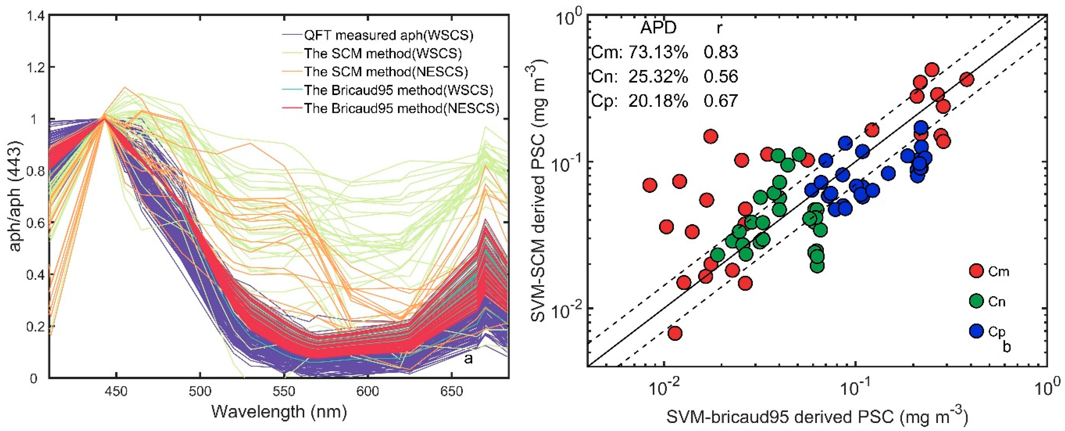
4.2. Errors from the Reconstruction of aph(λ)

Since obtaining aph(λ) is the other important part of the PSC model, the uncertainties introduced by the aph(λ) derived from at-w(λ) instead of aph(λ) measurements into the PSC model need to be evaluated. Due to the lack of match-ups of the measurements of at-w(λ) and aph(λ) in NESCS dataset, the accuracies of reconstructed aph(λ) derived from the Bricaud95 method and the SCM method were evaluated using the QFT measured aph(λ) in the WSCS dataset, which contained 114 match-ups. Later, the reconstructed aph(λ) were combined with the same reconstructed Chla as inputs to the SVM to control monospecific variability. The feasibility of the PSC methods in terms of reconstructing aph(λ) was evaluated by comparing the retrieved PSCs against in situ PSCs to evaluate the errors of the PSC model introduced using different reconstructed methods.
We compiled a dataset in the WSCS that contained nearshore and offshore in situ measurements of aph(λ) and at-w(λ) from AC-S observations in order to independently validate the reconstruction of aph(λ) using the Bricaud95 method and the SCM method. Figure 12 and Table 5 summarize the comparisons results and statistical parameters between aph(λ)/aph(443) derived from the two methods and in situ aph(λ)/aph(443) measurements. Generally, aph(λ)/aph(443) from the Bricaud95 method agreed better with measurements than those from the SCM method, with APD = 6.70% (412nm), 23.20% (490nm), 47.41% (510nm), 117.81% (555nm), and 64.72% (670nm) for the Bricaud95 method and APD = 23.70% (412nm), 71.25% (490nm), 159.51% (510nm), 609.62% (555nm), and 181.73% (670nm) for the SCM method. At 555 nm, the significant high errors in the derived of aph(555)/aph(443) from both methods were observed, which was associated with generally low or minimum magnitudes of aph(555) [48,49]. As Figure 12a shows, for the WSCS dataset, the spectral shapes of aph(λ)/aph(443) from the Bricaud95 method were also more in line with the measured aph(λ)/aph(443) spectra than those from the SCM method. Compared with the results for the WSCS dataset, the spectral shapes of aph(λ)/aph(443) derived from the two methods for the NESCS dataset generally follow the spectral variability for the WSCS dataset. Given the lack of the match-ups dataset in NESCS, the errors of the aph(λ)/aph(443) derived from two methods validated by the WSCS dataset would be approximately considered as the errors for NESCS dataset later.
To evaluate the effects of aph(λ) derived from the two methods instead of the measurements on retrievals of PSC model, we compared the PSC results derived using SVM-SCM and SVM-Bricaud95 for the NESCS dataset. Figure 12b shows the comparison of the PSC retrieved from SVM-SCM against those obtained from SVM-Bricaud95. Interestingly, these two types of PSC models revealed comparable performance with r ranging from 0.56 to 0.83. Cm from two types of PSC models presented the highest deviation with APD of 73.13%, while Cn and Cp showed relatively low deviations with APDs of 25.32% and 20.18%, respectively. Especially at low chlorophyll concentrations (<4 × 10⁻² mg∙m−3), the Cm from SVM-SCM was significantly higher than that from SVM-Bricaud95, and it also significantly deviated from in situ Cm values (as shown in Figure 7g). In general, the errors of reconstructed aph(λ) using the two methods led to 20– 70% errors in the PSC model.
Both methods performed poorly at retrieving Cm at low Chla. One possible reason is that the samples with low Chla were generally dominated by pico-phytoplankton in the NESCS dataset (Figure 3). In the case of the low magnitude of Cm, the small deviation in Cm from the PSC model might have presented the large relative error. This uncertainty in Cm prediction at lower Chla may have been driven by a reduced capability of the SVM. In addition, these deviations of spectral shapes derived from two methods might have led to the overestimation of Cm and the disagreements in Cm derived from these two methods. The samples dominated by micro-phytoplankton always had a high packaging effect and present a flat spectral shape of aph(λ), whereas pico-dominated samples generally had a low packaging effect and show a sharp spectral shape of aph(λ). As Figure 12b shows, the relatively flat spectrum of aph(λ) derived from the SCM method were closer to the spectra for micro-dominated samples. It might be another possible source of error for the overestimation of Cm at low Chla.
It must be pointed out that in SVM-Bricaud95, RChlaLH and aph(λ) were dependent, and aph(λ) were estimated from RChlaLH by Equation (7), while RChlaLH and aph(λ)/aph(443) spectra were independently decided in SVM-SCM. The PSCs derived from SVM-SCM was poorer than the SVM-Bricaud95 method, with APD values between 51% and 364.6%, and r2 ranging from 0.11 to 0.68. The main source of error from SVM-SCM may have been because inequality constraints used in the SCM model were determined using a global dataset, while the parameters in the Bricaud95 method were regionally fitted in our study area. Besides, the Bricaud95 method is based on three wavelengths of at-w(λ) longer than 650nm, which minimizes dependence on aCDOM(λ). Thus, to the extent possible, the effects of aCDOM(λ) contribution are avoided. Therefore, we recommend applying SVM-Bricaud95 to the vertical retrieval of PSCs at this stage. The Gaussian decomposition method provided the other effective way to reconstruct aph(λ) using several Gaussian functions from absorption by particles (ap(λ)) [61,62,63]. If there was aCDOM(λ) data in the AC-S dataset, vertical ap(λ) could be measured and then aph(λ) could be derived by this decomposition models. The impacts of the accuracy of reconstructed aph(λ) of the proposed PSC model cannot be ignored. The regional tuned SCM method and dataset contained AC-S measured vertical aCDOM(λ) data should be taken in our future works. Once the regionally tuned SCM and the Gaussian decomposition method are evaluated in SCS, these two methods can also provide other effective ways to retrieve vertical PSC in the future.

5. Conclusions

In this paper, we developed a regional PSC model to estimate the vertical PSC from the at-w(λ) and Chla. We first reconstructed Chla from at-w(λ) based on the aLH method. aph(λ) was further derived from Chla using the Bricaud95 method and directly from at-w(λ) using the SCM methods. Then, the SVM was trained based on in situ aph(λ) and Chla from the SCS dataset. Finally, the reconstructed aph(λ) and Chla were used as inputs to an SVM to retrieve vertical PSCs. The developed PSC model was tested on a dataset from the SCS dataset and validated using an independent dataset from the NESCS Cruise.
The sensitivities of the selection of optical inputs, and the random splitting ratio of the training and test datasets were executed. The results show that the SVM using aph(λ)/ aph(443) and in situ Chla as inputs performed well. Moreover, randomly splitting the data into training and test datasets with ratios of 80% and 20% was reasonable. Moreover, the SVM was insensitive to randomly picked datasets. The performance of PSC was affected by the accuracy of reconstructed aph(λ) and Chla. The accuracy of reconstructed Chla were in good agreement with in situ measurement of Chla, with r2 and APD values of 0.77 and 58%, respectively. The accuracy of reconstructed aph(λ) at the wavelength of 412nm, 490nm, 510nm, 555nm, and 670nm had APDs of 6.70%, 23.20%, 47.41%, 117.81%, and 64.72% for the Bricaud95 method and 23.70%, 71.25%, 159.51%, 609.62%, and 181.73% for the SCM method, respectively. Influences introduced in the PSC model via in replacement of the reconstructed Chla with in situ Chla was evaluated to show that the substitution could improve the PSC model performance, decreasing APD to between 37% and 52%. The regional PSC model was also compared with the tuned three-component models, and the results suggest that the former outperformed the latter, with APD values lowered to between 81.1% and 190.2%. At low concentration, the Cm retrieval could lead to large deviations due to shortcomings of the model.
One appeal of the PSC model is that it does not require in situ measurement of Chla, and can be used to retrieve vertical high depth resolution PSCs along the transection using only absorption data from continuous profiling systems (e.g., WET Labs AC-S). Our PSC model actually provides a faster retrieval of vertical PSC and the possibility to obtain the PSC with a fine vertical resolution within the water column.

Author Contributions

All authors conceived and designed the study. Conceptualization, L.D., W.Z. (Wen Zhou) and W.C.; Writing-Original Draft Preparation, L.D.; Writing-Review & Editing, L.D., W.Z. (Wen Zhou) and W.C.; Methodology, G.W. and W.Z. (Wen Zhou); Investigation, S.H., W.Z. (Wenjing Zhao) and Z.X.; Software, L.D. and W.Z. (Wendi Zheng). Funding Acquisition, W.C., Y.Y., C.L. and W.Z. (Wen Zhou).

Funding

This work was funded by National Natural Science Foundation of China (41431176, 41576030, 41367042, 41776045, and 41776044); the Science and Technology Planning Project of Guangdong Province, China (2016A020222008); the Science and Technology Planning Project of Guangzhou, China (201504010034, 201607020041, and 201707020023); the China Scholarship Council; The Strategic Priority Research Program of the Chinese Academy of Sciences (XDA11040302); and the Open Project Program of the State Key Laboratory of Tropical Oceanography (No. LTOZZ1602).

Acknowledgments

We thank all scientists and personnel who contributed to the collection and processing of field data used in this study. In particular, we thank G. Zheng who provided the code for the stacked constraints model.

Conflicts of Interest

The authors declare no conflict of interest.

References

  1. Falkowski, P.G.; Katz, M.E.; Knoll, A.H.; Quigg, A.; Raven, J.A.; Schofield, O.; Taylor, F.J. The evolution of modern eukaryotic phytoplankton. Science 2004, 305, 354–360. [Google Scholar] [CrossRef] [PubMed]
  2. Field, C.; Behrenfeld, M.; Randerson, J.; Falkowsk, P. Primary Production of the Biosphere: Integrating Terrestrial and Oceanic Components. Science 1998, 281, 237–240. [Google Scholar] [CrossRef]
  3. Longhurst, A.; Sathyendranath, S.; Platt, T.; Caverhill, C. An estimate of global primary production in the ocean from satellite radiometer data. J. Plank. Res. 1995, 17, 1245–1271. [Google Scholar] [CrossRef]
  4. Le Quéré, C.; Harrison, S.P.; Prentice, C.I.; Buitenhuis, E.T.; Aumont, O.; Bopp, L.; Claustre, H. Ecosystem dynamics based on plankton functional types for global ocean biogeochemistry models. Glob. Change Bio. 2005, 11, 2016–2040. [Google Scholar] [CrossRef]
  5. Geider, R.J.; Platt, T.; Raven, J.A. Size dependence of growth and photosynthesis in diatoms: A synthesis. Mar. Ecol. Prog. Ser. 1986, 30, 93–104. [Google Scholar] [CrossRef]
  6. Maloney, C.L.; Field, J.G. The size-based dynamics of plankton food webs. I. A simulation model of carbon and nitrogen flows. J. Plank. Res. 1991, 13, 1003–1038. [Google Scholar] [CrossRef]
  7. Parsons, T.R.; Lalli, C.M. Jellyfish populations explosions: Revisiting a hypothesis of possible causes. La Mer 2002, 40, 640–647. [Google Scholar]
  8. Platt, T.; Denman, K.L. The relationship between photosynthesis and light for natural assemblages of coastal marine phytoplankton. J. Phyco. 1976, 12, 421–430. [Google Scholar] [CrossRef]
  9. Probyn, T.A. Nitrogen uptake by size-fractionated phytoplankton populations in the southern Benguela upwelling system. Mar. Ecol. Prog. Ser. 1985, 22, 249–258. [Google Scholar] [CrossRef]
  10. Sieburth, J.; Smetacek, V.; Lenz, J. Pelagic ecosystem structure: Heterotrophic compartments of the plankton and their relationship to plankton size fraction. Limnol. Oceanogr. 1978, 23, 1256–1263. [Google Scholar] [CrossRef]
  11. IOCCG. Phytoplankton Functional Types from Space. In Reports of the International Ocean-Colour Coordinating Group; Sathyendranath, S., Ed.; IOCCG: Dartmouth, NS, Canada, 2014. [Google Scholar]
  12. Brewin, R.; Sathyendranath, S.; Hirata, T.; Lavender, S.J.; Barciela, R.M.; Hardman-Mountford, N.J. A three-component model of phytoplankton size class for the Atlantic Ocean. Ecol. Model. 2010, 221, 1472–1483. [Google Scholar] [CrossRef]
  13. Hirata, T.; Hardman-Mountford, N.J.; Brewin, R.J.W.; Aiken, J.; Barlow, R.; Suzuki, K.; Isada, T.; Howell, E.; Hashioka, T.; Noguchi-Aita, M.; et al. Synoptic relationships between surface Chlorophyll-a and diagnostic pigments specific to phytoplankton functional types. Biogeosci. 2011, 8, 311–327. [Google Scholar] [CrossRef]
  14. Sathyendranath, S.; Cota, G.; Stuart, V.; Maass, H.; Platt, T. Remote sensing of phytoplankton pigments: A comparison of empirical and theoretical approaches. Int. J. Remote Sens. 2001, 22, 249–273. [Google Scholar] [CrossRef]
  15. Uitz, J.; Claustre, H.; Morel, A.; Hooker, S.B. Vertical distribution of phytoplankton communities in open ocean: An assessment based on surface chlorophyll. J. Geophys. Res. 2006, 111. [Google Scholar] [CrossRef]
  16. Ciotti, A.; Bricaud, A. Retrievals of a size parameter for phytoplankton and spectral light absorption by coloured detrital matter from water-leaving radiances at SeaWiFS channels in a continental shelf off Brazil. Limnol. Oceanogr. 2006, 4, 237–253. [Google Scholar] [CrossRef]
  17. Ciotti, A.; Lewis, M.R.; Cullen, J.J. Assessment of the Relationships between Dominant Cell Size in Natural Phytoplankton Communities and the Spectral Shape of the Absorption Coefficient. Limnol. Oceanogr. 2002, 47, 404–417. [Google Scholar] [CrossRef]
  18. Devred, E.; Sathyendranath, S.; Stuart, V.; Maass, H.; Ulloa, O.; Platt, T. A two-component model of phytoplankton absorption in the open ocean: Theory and applications. J. Geophys. Res. 2006, 111. [Google Scholar] [CrossRef]
  19. Hirata, T.; Aiken, J.; Hardman-Mountford, N.; Smyth, T.J.; Barlow, R.G. An absorption model to determine phytoplankton size classes from satellite ocean colour. Remote Sens. Environ. 2008, 112, 3153–3159. [Google Scholar] [CrossRef]
  20. Roy, S.; Sathyendranath, S.; Bouman, H.; Platt, T. The global distribution of phytoplankton size spectrum and size classes from their light-absorption spectra derived from satellite data. Remote Sens. Environ. 2013, 139, 185–197. [Google Scholar] [CrossRef]
  21. Kostadinov, T.S.; Siegel, D.A.; Maritorena, S. Retrieval of the particle size distribution from satellite ocean color observations. J. Geophys. Res. 2009, 114, 1–22. [Google Scholar] [CrossRef]
  22. Emanuele, O.; Annick, B.; David, A.; Julia, U. Multivariate approach for the retrieval of phytoplankton size structure from measured light absorption spectra in the Mediterranean Sea. Appl. Opt. 2013, 52, 2257–2273. [Google Scholar]
  23. Wang, S.; Ishizaka, J.; Hirawake, T.; Watanabe, Y.; Zhu, Y.; Hayashi, M.; Yoo, S. Remote estimation of phytoplankton size fractions using the spectral shape of light absorption. Opt. Express 2015, 23, 10301–10318. [Google Scholar] [CrossRef]
  24. Catlett, D.; Siegel, D.A. Phytoplankton Pigment Communities Can be Modeled Using Unique Relationships with Spectral Absorption Signatures in a Dynamic Coastal Environment. J. Geophys. Res. 2018, 123, 246–264. [Google Scholar] [CrossRef]
  25. Torrecilla, E.; Stramski, D.; Reynolds, R.A.; Millán-Núñez, E.; Piera, J. Cluster analysis of hyperspectral optical data for discriminating phytoplankton pigment assemblages in the open ocean. Remote Sens. Environ. 2011, 115, 2578–2593. [Google Scholar] [CrossRef]
  26. Uitz, J.; Stramski, D.; Reynolds, R.A.; Dubranna, J. Assessing phytoplankton community composition from hyperspectral measurements of phytoplankton absorption coefficient and remote-sensing reflectance in open-ocean environments. Remote Sens. Environ. 2015, 171, 58–74. [Google Scholar] [CrossRef]
  27. Brewin, R.J.W.; Hardman-Mountford, N.J.; Lavender, S.J.; Raitsos, D.E.; Hirata, T.; Uitz, J.; Devred, E.; Bricaud, A.; Ciotti, A.; Gentili, B. An intercomparison of bio-optical techniques for detecting dominant phytoplankton size class from satellite remote sensing. Remote Sens. Environ. 2011, 115, 325–339. [Google Scholar] [CrossRef]
  28. Raitsos, D.E.; Lavender, S.J.; Maravelias, C.D.; Haralambous, J.; Richardson, A.J.; Reid, P.C. Identifying phytoplankton functional groups from space: An ecological approach. Limnol. Oceanogr. 2008, 53, 605–613. [Google Scholar] [CrossRef]
  29. Li, Z.; Li, L.; Song, K.; Cassar, N. Estimation of phytoplankton size fractions based on spectral features of remote sensing ocean color data. J. Geophys. Res. 2013, 118, 1445–1458. [Google Scholar] [CrossRef]
  30. Hu, S.; Liu, H.; Zhao, W.; Shi, T.; Hu, Z.; Li, Q.; Wu, G. Comparison of Machine Learning Techniques in Inferring Phytoplankton Size Classes. Remote Sens. 2018, 10. [Google Scholar] [CrossRef]
  31. Brewin, R.J.W.; Hirata, T.; Hardman-Mountford, N.J.; Lavender, S.J.; Sathyendranath, S.; Barlow, R. The influence of the Indian Ocean Dipole on interannual variations in phytoplankton size structure as revealed by Earth Observation. Deep Sea Res. II 2012, 77–80, 117–127. [Google Scholar] [CrossRef]
  32. Mouw, C.B.; Yoder, J.A. Optical determination of phytoplankton size composition from global SeaWiFS imagery. J. Geophys. Res. 2010, 115. [Google Scholar] [CrossRef]
  33. Nair, A.; Sathyendranath, S.; Platt, T.; Morales, J.; Stuart, V.; Forget, M.-H.; Devred, E.; Bouman, H. Remote sensing of phytoplankton functional types. Remote Sens. Environ. 2008, 112, 3366–3375. [Google Scholar] [CrossRef]
  34. Dai, M.; Zhai, W.; Cai, W.-J.; Callahan, J.; Huang, B.; Shang, S.; Huang, T.; Li, X.; Lu, Z.; Chen, W.; et al. Effects of an estuarine plume-associated bloom on the carbonate system in the lower reaches of the Pearl River estuary and the coastal zone of the northern South China Sea. Cont. Shelf Res. 2008, 28, 1416–1423. [Google Scholar] [CrossRef]
  35. Mitchell, B.G. Algorithms for determining the absorption coefficient of aquatic particulates using the quantitative filter technique (QFT). SPIE 1990, 1302, 137–148. [Google Scholar]
  36. Yentsch, C.S. Measurement of Visible Light Absorption by Particulate Matter in the Ocean. Limnol. Oceanogr. 1962, 7, 207–217. [Google Scholar] [CrossRef]
  37. Kisino, M.; Takahashi, M.; Okami, N.; Ichimura, S. Estimation of the spectral absorption coefficients of phytoplankton in the sea. Bull. Mar. Sci. 1985, 37, 634–642. [Google Scholar]
  38. Babin, M.; Stramski, D.; Ferrari, G.; Claustre, H.; Bricaud, A.; Obolensky, G.; Hoepffner, N. Variations in the light absorption coefficients of phytoplankton, nonalgal particles, and dissolved organic matter in coastal waters around Europe. J. Geophys. Res. 2003, 108. [Google Scholar] [CrossRef]
  39. Bricaud, A.; Morel, A.; Babin, M.; Allali, K.; Claustre, H. Variations of light absorption by suspended particles with chlorophyllaconcentration in oceanic (case 1) waters: Analysis and implications for bio-optical models. J. Geophys. Res. 1998, 103, 31033–31044. [Google Scholar] [CrossRef]
  40. Bricaud, A.; Stramski, D. Spectral absorption coefficients of living phytoplankton and nonalgal biogenous matter: A comparison between the Peru upwelling area and the Sargasso Sea. Limnol. Oceanogr. 1990, 35, 562–582. [Google Scholar] [CrossRef]
  41. Roesler, C.S. Theoretical and experimental approaches to improve the accuracy of particulate absorption coefficients from the Quantitative Filter Technique. Limnol. Oceanogr. 1998, 43, 11. [Google Scholar] [CrossRef]
  42. Vidussi, F.; Claustre, H.; Manca, B.B.; Luchetta, A.; Marty, J.-C. Phytoplankton pigment distribution in relation to upper thermocline circulation in the eastern Mediterranean Sea during winter. J. Geophys. Res. 2001, 106, 19939–19956. [Google Scholar] [CrossRef]
  43. Sullivan, J.; Twardowski, M.; Zaneveld, J.R.V.; Moore, C.; Barnard, A.H.; Donaghay, P.L.; Rhoades, B. Hyperspectral temperature and salt dependencies of absorption by water and heavy water in the 400–750 nm spectral range. Appl. Opt. 2006, 45, 5294–5309. [Google Scholar] [CrossRef]
  44. Zaneveld, J.R.V.; Kitchen, J.C.; Moore, C.C. Scattering error correction of reflecting-tube absorption meters. SPIE Ocean Opt. XII 1994, 2258, 44–55. [Google Scholar]
  45. Claustre, H. The Trophic Status of Various Oceanic Provinces as Revealed by Phytoplankton Pigment Signatures. Limnol. Oceanogr. 1994, 39, 1206–1210. [Google Scholar] [CrossRef]
  46. Roesler, C.S.; Barnard, A.H. Optical proxy for phytoplankton biomass in the absence of photophysiology: Rethinking the absorption line height. Methods in Oceanogr. 2013, 7, 79–94. [Google Scholar] [CrossRef]
  47. Bricaud, A.; Babin, M.; Morel, A.; Claustre, H. Variability in the chlorophyll-specific absorption coefficients of natural phytoplankton: Analysis and parameterization. J. Geophys. Res. 1995, 100, 13321. [Google Scholar] [CrossRef]
  48. Zheng, G.; Stramski, D. A model based on stacked-constraints approach for partitioning the light absorption coefficient of seawater into phytoplankton and non-phytoplankton components. J. Geophys. Res. 2013, 118, 2155–2174. [Google Scholar] [CrossRef]
  49. Zheng, G.; Stramski, D.; DiGiacomo, P.M. A model for partitioning the light absorption coefficient of natural waters into phytoplankton, nonalgal particulate, and colored dissolved organic components: A case study for the Chesapeake Bay. J. Geophys. Res. 2015, 120, 2601–2621. [Google Scholar] [CrossRef]
  50. Boss, E.S.; Collier, R.; Larson, G.; Fennel, K.; Pegau, W.S. Measurements of spectral optical properties and their relation to biogeochemical variables and processes in Crater Lake, Crater Lake National Park, OR. Hydrobiology 2007, 574, 149–159. [Google Scholar] [CrossRef]
  51. Boss, E.; Picheral, M.; Leeuw, T.; Chase, A.; Karsenti, E.; Gorsky, G.; Taylor, L.; Slade, W.; Ras, J.; Claustre, H. The characteristics of particulate absorption, scattering and attenuation coefficients in the surface ocean; Contribution of the Tara Oceans expedition. Methods Oceanogr. 2013, 7, 52–62. [Google Scholar] [CrossRef]
  52. Lin, J.; Cao, W.; Zhou, W.; Sun, Z.; Xu, Z.; Wang, G.; Hu, S. Novel method for quantifying the cell size of marine phytoplankton based on optical measurements. Opt. Express 2014, 22, 10467–10476. [Google Scholar] [CrossRef] [PubMed]
  53. Lamont, T.; Barlow, R.; Brewin, R. Variations in Remotely-Sensed Phytoplankton Size Structure of a Cyclonic Eddy in the Southwest Indian Ocean. Remote Sens. 2018, 10. [Google Scholar] [CrossRef]
  54. Sahay, A.; Ali, S.M.; Gupta, A.; Goes, J.I. Ocean color satellite determinations of phytoplankton size class in the Arabian Sea during the winter monsoon. Remote Sens. Environ. 2017, 198, 286–296. [Google Scholar] [CrossRef]
  55. Varunan, T.; Shanmugam, P. A model for estimating size-fractioned phytoplankton absorption coefficients in coastal and oceanic waters from satellite data. Remote Sens. Environ. 2015, 158, 235–254. [Google Scholar] [CrossRef]
  56. Hu, S.; Zhou, W.; Wang, G.; Cao, W.; Xu, Z.; Liu, H.; Wu, G.; Zhao, W. Comparison of Satellite-Derived Phytoplankton Size Classes Using In-Situ Measurements in the South China Sea. Remote Sens. 2018, 10. [Google Scholar] [CrossRef]
  57. Zhang, H.; Wang, S.; Qiu, Z.; Sun, D.; Ishizaka, J.; Sun, S.; He, Y. Phytoplankton size class in the East China Sea derived from MODIS satellite data. Biogeoscience 2018, 15, 4271–4289. [Google Scholar] [CrossRef]
  58. Lin, J.; Cao, W.; Zhou, W.; Hu, S.; Wang, G.; Sun, Z.; Xu, Z.; Song, Q. A bio-optical inversion model to retrieve absorption contributions and phytoplankton size structure from total minus water spectral absorption using genetic algorithm. Chin. J. Ocean Limnol. 2013, 31, 970–978. [Google Scholar] [CrossRef]
  59. Huang, B.; Hu, J.; Xu, H.; Cao, Z.; Wang, D. Phytoplankton community at warm eddies in the northern South China Sea in winter 2003/2004. Deep Sea Res. II 2010, 57, 1792–1798. [Google Scholar] [CrossRef]
  60. Waga, H.; Hirawake, T.; Fujiwara, A.; Kikuchi, T.; Nishino, S.; Suzuki, K.; Takao, S.; Saitoh, S.-I. Differences in Rate and Direction of Shifts between Phytoplankton Size Structure and Sea Surface Temperature. Remote Sens. 2017, 9. [Google Scholar] [CrossRef]
  61. Chase, A.; Boss, E.; Zaneveld, R.; Bricaud, A.; Claustre, H.; Ras, J.; Dall’Olmo, G.; Westberry, T.K. Decomposition of in situ particulate absorption spectra. Methods Oceanogr. 2013, 7, 110–124. [Google Scholar] [CrossRef]
  62. Hoepffner, N.; Sathyendranath, S. Effect of pigment composition on absorption properties of phytoplankton. Mar. Ecol. Prog. Ser. 1991, 73, 11–23. [Google Scholar] [CrossRef]
  63. Hoepffner, N.; Sathyendranath, S. Determination of the major groups of phytoplankton pigments from the absorption spectra of total particulate matter. J. Geophys. Res. 1993, 98. [Google Scholar] [CrossRef]
Figure 1. Locations of SCS dataset (purple square), NESCS dataset (red circle), WSCS dataset (yellow circle), the transect-A (green triangle), and Station 50 (cyan triangle). The upward direction is due north.
Remotesensing 11 01054 g001
Figure 2. Schematic of regional PSC model building and steps of application.
Remotesensing 11 01054 g002
Figure 3. Ternary plots showing the fm, fn, and fp of SCS and NESCS datasets.
Remotesensing 11 01054 g003
Figure 4. Boxplot of retrieved PSCs for three inputs (red, green, and blue represent SVM-Type1, SVM-Type2, and SVM-Type3, respectively) for (a) the training dataset and (b) the test dataset.
Remotesensing 11 01054 g004
Figure 5. Cross-validation of splitting the data into training and testing datasets. (a) Absolute percentage differences (in %) of model derived for PSCs with respect to ratio of training dataset. (b) Coefficient of determination of the derived PSCs with respect to ratio of training dataset. The broken lines indicate the test dataset. Red, green, and blue represent Cm, Cn, and Cp, respectively.
Remotesensing 11 01054 g005
Figure 6. Cross-validation of random pick tests. (a) Absolute percentage differences (in %) of randomly picked training and test datasets in estimation of PSC with respect to statistic quartiles. (b) Coefficient of determination of randomly picked training and test datasets in the estimation of PSC with respect to statistic quartiles. The straight lines indicate the training datasets and broken lines indicate the test dataset. The dotted lines represent the statistical locations of the first and third quartiles. Red, green, and blue represent Cm, Cn, and Cp, respectively.
Remotesensing 11 01054 g006
Figure 7. Scatter plots of the PSC derived from the model against in situ PSC. (a,b,c) The scatter plots of the training dataset. (d,e,f) The scatter plots of the test dataset. (g,h,i) The scatter plots of SVM-SCM applied to the NESCS dataset. (j,k,l) The scatter plots of SVM-Bricaud95 applied to the NESCS dataset. The black line represents the 1:1 line and dotted lines represent the 1:1 line ± 30% log10 PSC.
Remotesensing 11 01054 g007
Figure 8. The vertical distribution of PSC and Chla retrieved by SVM-Bricaud95 at Station 50. The solid circles represent the PSC measured using the HPLC method. The open circles represent the profile PSC derived from SVM-Bricaud95. The dotted lines represent the range within one-fold APD.
Remotesensing 11 01054 g008
Figure 9. Vertical distribution along transect-A of the concentrations of total chlorophyll (a), and the proportions of micro- (b), nano- (c), and pico-phytoplankton (d), respectively.
Remotesensing 11 01054 g009
Figure 10. (a) Fitted curve and scatter plots between aLH(676) and Chla of NESCS dataset. (b) Scatter plots of RChlaLH and in situ Chla. The black line represents the 1:1 line and the dotted lines represent the 1:1 line ± 30% log10 PSC.
Remotesensing 11 01054 g010
Figure 11. Scatter plots of PSC retrieved using SVM-Bricaud95 and SVM-Bricaud95 (in situ Chla) for (a) Cm, (b) Cn, and (c) Cp. Scatter plots of SVM-Bricaud95 and SVM-Bricaud95 (in situ Chla) (open circle) versus (solid circle) (d). The black line represents the 1:1 line and the dotted lines represent the 1:1 line ± 30% log10 PSC.
Remotesensing 11 01054 g011
Figure 12. Scatter plots of PSC derived using SVM-SCM PSC versus SVM-Bricaud95 (a). aph(443)-specific absorption coefficients of phytoplankton reconstructed by Bricaud95 methods (b). Black line represents the 1:1 line and dotted lines represent the 1:1 line ± 30% log10 PSC.
Remotesensing 11 01054 g012
Table 1. Summary of datasets used in this study.
Data Type and Number of Points
TrainingTestApplyValidate
ExpeditionCruise PeriodLocationsHPLC and aph(λ) HPLC and aph(λ) HPLC and at-w(λ)at-w(λ) and aph(λ)Totals
SCSSeptember 2006–August 2013South China Sea33483 417
NESCS5–17 August 2015Northeast South China Sea 52 52
WSCS9 August–2 September 2013
1–23 October 2017
North South China Sea 114114
Table 2. Statistical parameters of PSCs derived from PSC models using three inputs.
Input ModelsSizeTrainTest
RMSAPD%RPD%r2RMSAPD%RPD%r2
SVM-Type1pico0.049615.154.260.880.040727.738.730.37
nano0.037425.648.760.640.015464.8539.860.66
micro0.102932.2010.340.950.011763.0835.960.43
SVM-Type2pico0.065235.7919.130.800.065226.990.290.80
nano0.037028.098.060.580.037945.0522.280.68
micro0.177135.2411.770.900.048550.1421.600.62
SVM-Type3pico0.065514.887.190.800.079439.8313.890.68
nano0.038731.449.420.560.038557.7134.140.59
micro0.116638.5313.290.940.080058.0923.890.87
Table 3. Statistics of the three models used to retrieve PSC.
ModelsSize ClassRMSAPD%RPD%r2
Three-component modelmicro0.2462295.6288.30.66
nano0.0630262.5204.80.28
pico0.228154.945.0510.53
SVM-Bricaud95 micro0.0981105.456.70.66
nano0.0740181.4960.35
pico0.251656.2818.810.57
SVM-SCMmicro0.1077364.6 326.70.68
nano0.0558262.2195.30.11
pico0.337251.9738.990.39
Table 4. Regionally tuned and default parameters of the three-component model.
C p , n m S p , n C p m S p
This paper0.3193.0180.2552.466
Brewin et al. (2010)0.7751.1520.1465.118
Table 5. Statistics of the Bricaud95-method and the SCM-method derived aph(λ)/aph(443).
VariableBricaud95SCM
RMSAPD%MRRMSAPD%MR
aph(λ)/aph(412)0.06856.700.990.240223.700.79
aph(λ)/aph(490)0.132423.201.230.421871.251.66
aph(λ)/aph(510)0.134047.411.460.5146159.512.47
aph(λ)/aph(555)0.0726117.811.770.5863609.627.36
aph(λ)/aph(670)0.179364.721.550.5142181.732.64

