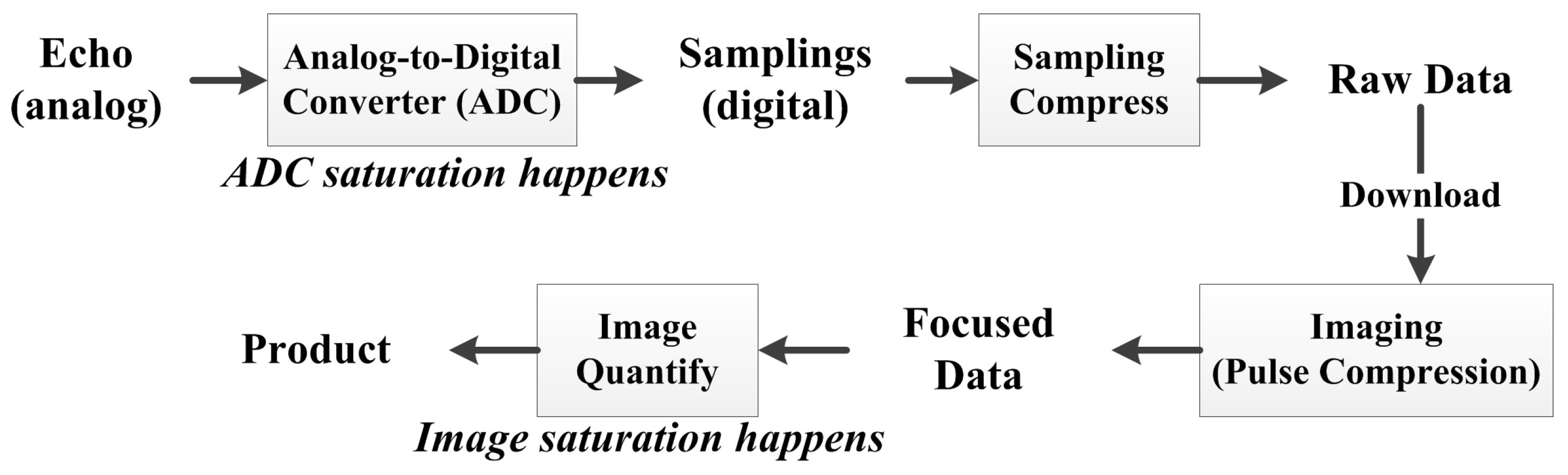
Figure 1.
Data flow of the synthetic aperture radar (SAR) system.
Figure 1.
Data flow of the synthetic aperture radar (SAR) system.
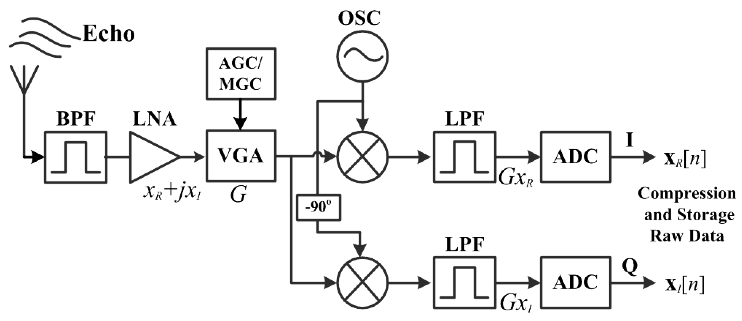
Figure 2.
Simple diagram of a radar receiver. BPF stands for Berkeley Packet Filter. LNA stands for Low-Noise Amplifier. AGC stands for Automatic Gain Controller. MGC stands for Manual Gain Controller. VGA stands for Variable Gain Amplifier. OSC stands for Open Source Commerce. LPF stands for Low-Pass Filter.
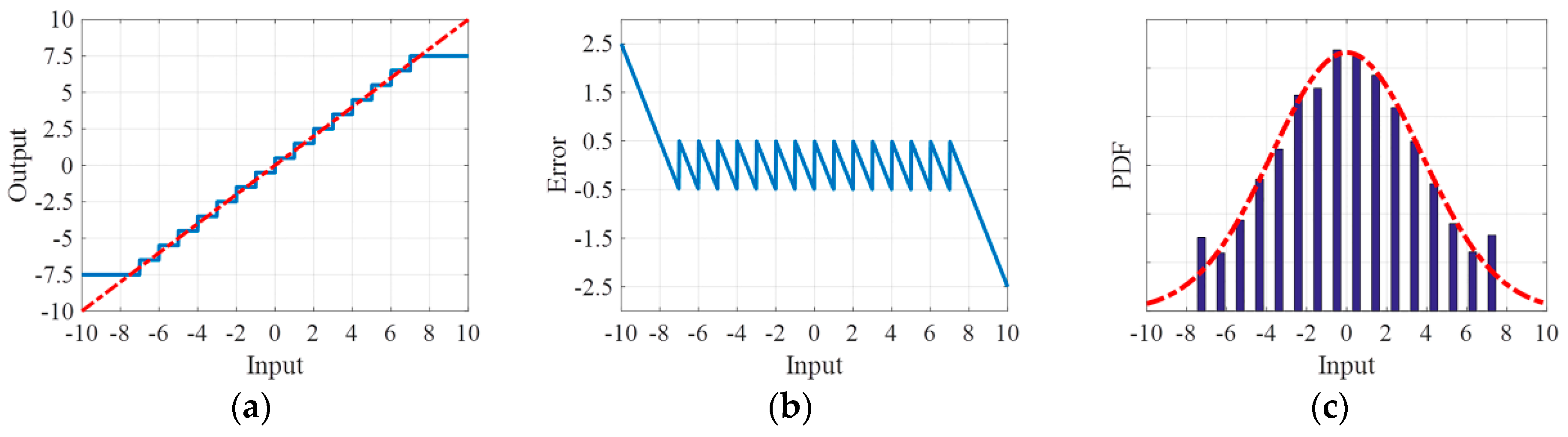
Figure 3.
ADC at 4-bits of quantization. (a) The dotted line indicates the input analog signal, and the solid line indicates the output digital signal. Values exceeding ±7.5 are set to the threshold, the continuous values are discretized. (b) The quantization error from the values within the threshold range is between ±0.5, and the saturation error is always larger than the quantization error. (c) The continuous Gaussian probability distribution (dotted line) becomes discrete (histogram).
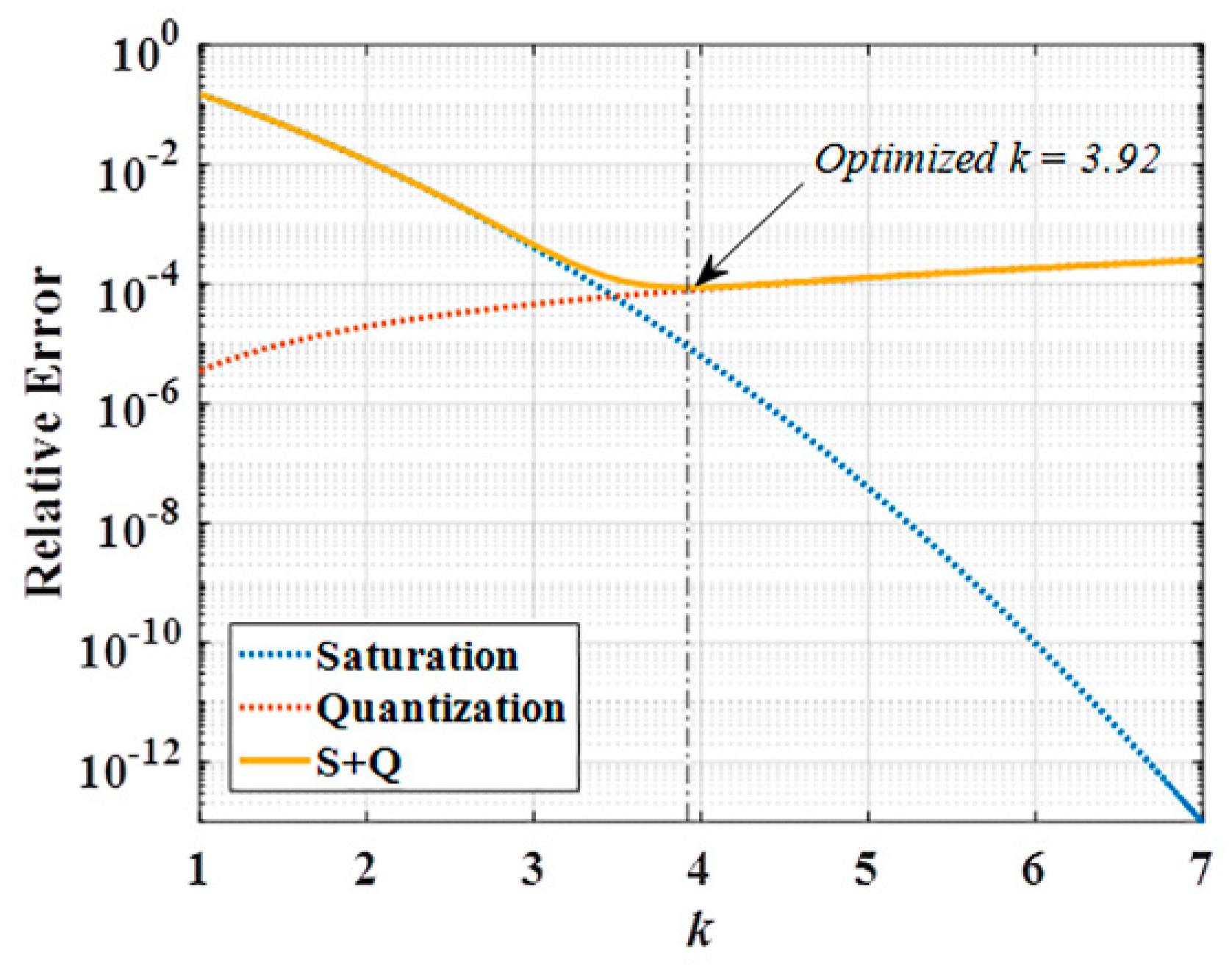
Figure 4.
The relative noise of quantization and saturation at 8-bits. The ADC error is dominated by saturation or quantization noise when variable is lower or higher than the optimum value, respectively.
Figure 4.
The relative noise of quantization and saturation at 8-bits. The ADC error is dominated by saturation or quantization noise when variable is lower or higher than the optimum value, respectively.
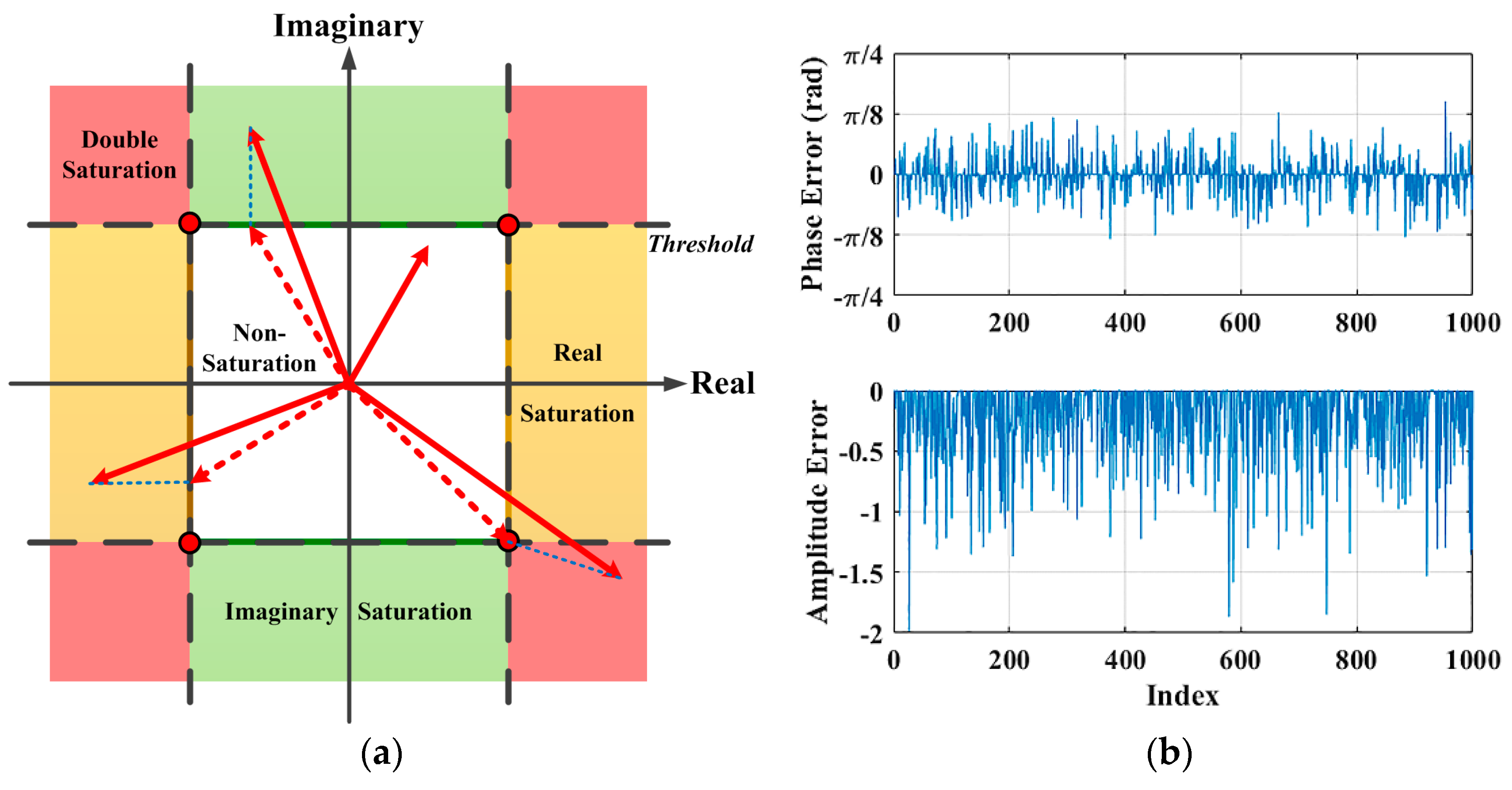
Figure 5.
Phase and amplitude errors of raw data samples. (a) The solid red lines are input vectors, and the dotted red lines are outputs with ADC saturation. If the samples fall in the white area, there is no saturation at all. In the yellow area or green area, there is only real or imaginary saturation, and the output values are set on the four edges of the white square nearby. If the samples fall within the red area, saturation occurs in both the real and imaginary parts, and the output values are all set at the four red corners. (b) The phase errors and amplitude errors of a zero-mean complex Gaussian echo with a clipping factor of 30% and normalized mean power.
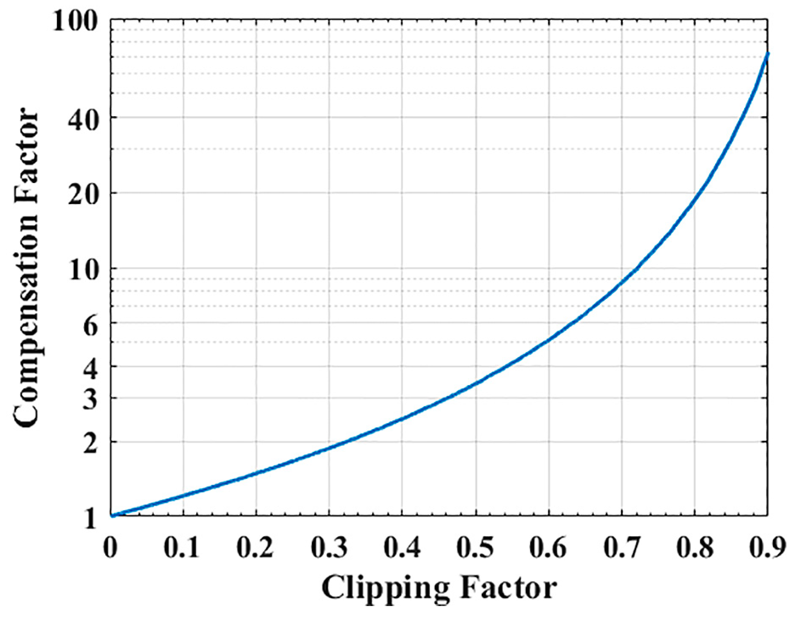
Figure 6.
Compensation factor for the power loss of focused data, which is caused by the saturation of raw data. The clipping factor is calculated in saturated raw data, the real and imaginary parts of which follow a zero-mean Gaussian distribution.
Figure 6.
Compensation factor for the power loss of focused data, which is caused by the saturation of raw data. The clipping factor is calculated in saturated raw data, the real and imaginary parts of which follow a zero-mean Gaussian distribution.
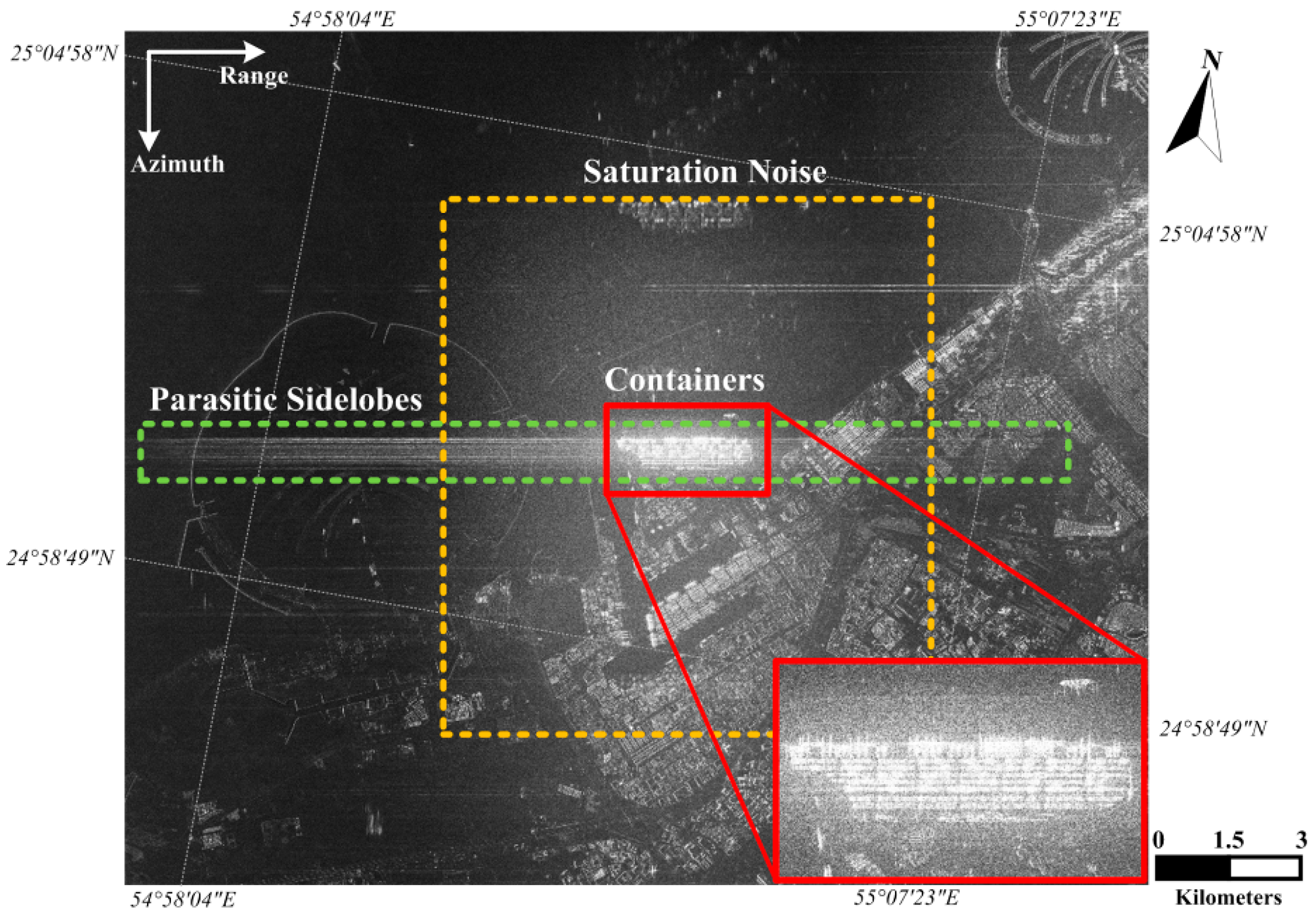
Figure 7.
The saturation of extremely strong targets in a Radarsat-2 image of Dubai. There is a container terminal at the center of the image. The placement direction of the containers (in the red rectangle) is perpendicular to the azimuth direction. Thus, the scattering intensity in this area is significantly higher than that in the remainder of the image.
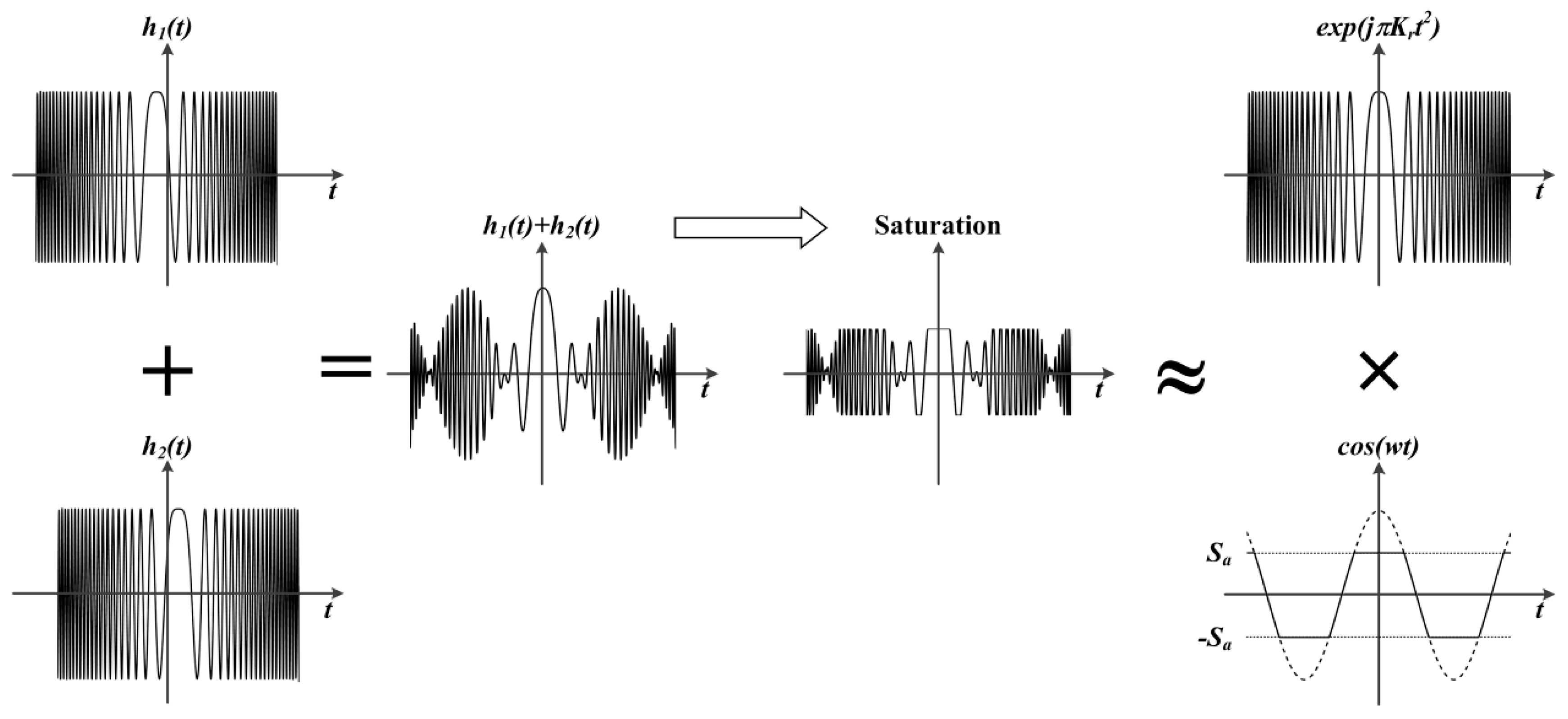
Figure 8.
The decomposition of the raw data between two points. Saturation mainly affects the periodic envelope.
Figure 8.
The decomposition of the raw data between two points. Saturation mainly affects the periodic envelope.
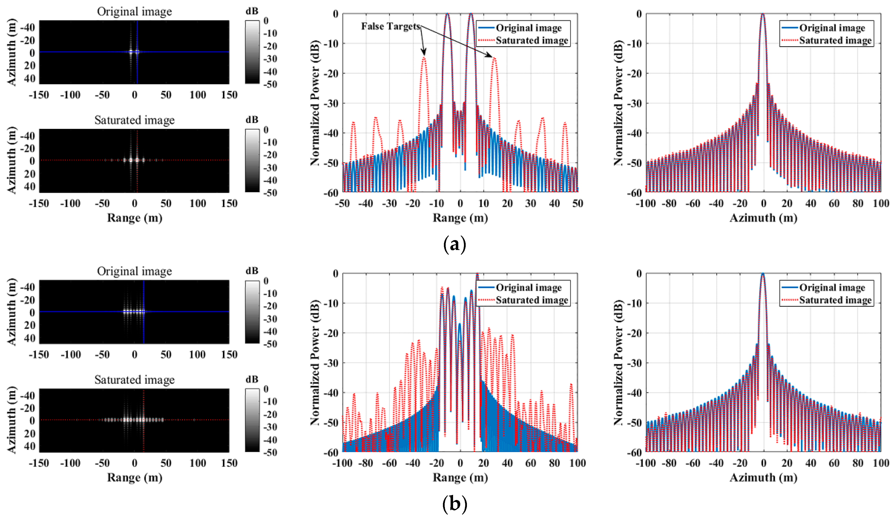
Figure 9.
Normalized imaging results for saturated raw data. The traditional sidelobes are suppressed by the Hamming window. (a) Two point targets cause false images. The main lobes of the real targets exhibit no significant degradation. (b) A series of isolated points result in a parasitic sidelobe.
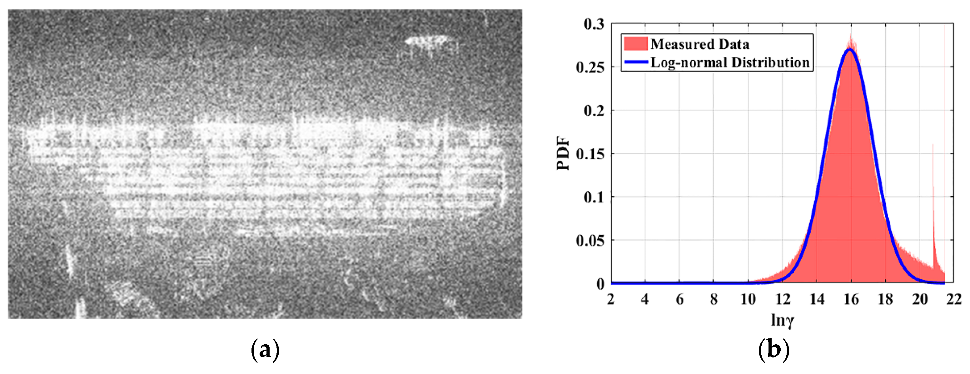
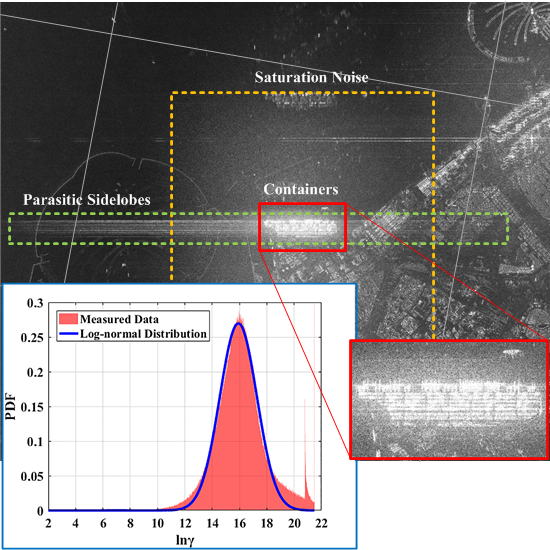
Figure 10.
Statistical result for containers. (a) The saturated area with isolated large dynamic range objects. (b) Fitting result for the energy associated with the containers. The two spikes at and are caused by the quantization threshold of the 16-bit complex image.
Figure 10.
Statistical result for containers. (a) The saturated area with isolated large dynamic range objects. (b) Fitting result for the energy associated with the containers. The two spikes at and are caused by the quantization threshold of the 16-bit complex image.
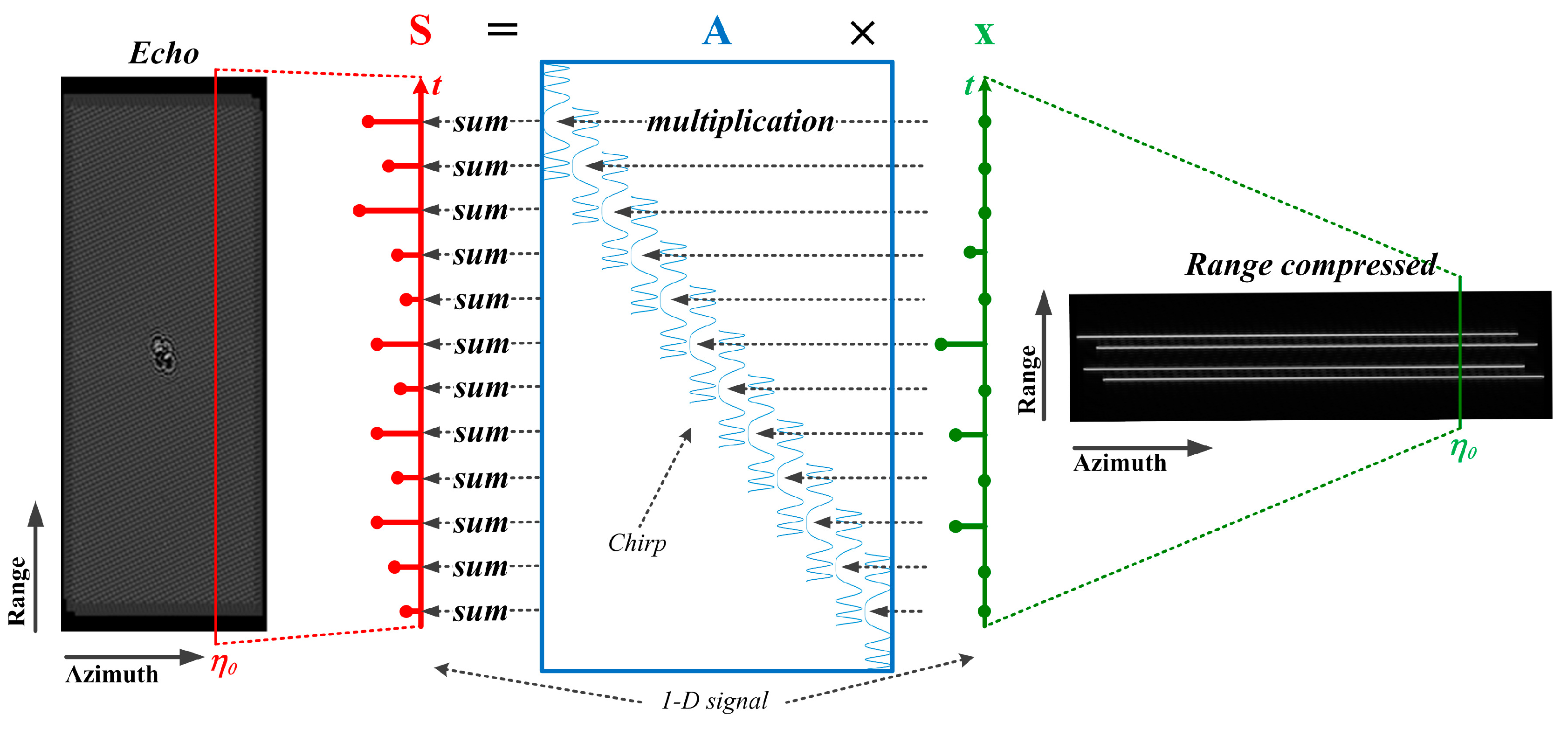
Figure 11.
The relationship between and . There are four point targets at the center of the scene, the echo of which spreads over a wide area, and the range compressed result is four lines. After range migration correction and azimuth compression, we can obtain the focused data.
Figure 11.
The relationship between and . There are four point targets at the center of the scene, the echo of which spreads over a wide area, and the range compressed result is four lines. After range migration correction and azimuth compression, we can obtain the focused data.
Figure 12.
The separation of matrix according to the saturation of signal . All green rows were recombined into matrix , and the red and yellow ones were recombined into matrices and respectively.
Figure 12.
The separation of matrix according to the saturation of signal . All green rows were recombined into matrix , and the red and yellow ones were recombined into matrices and respectively.
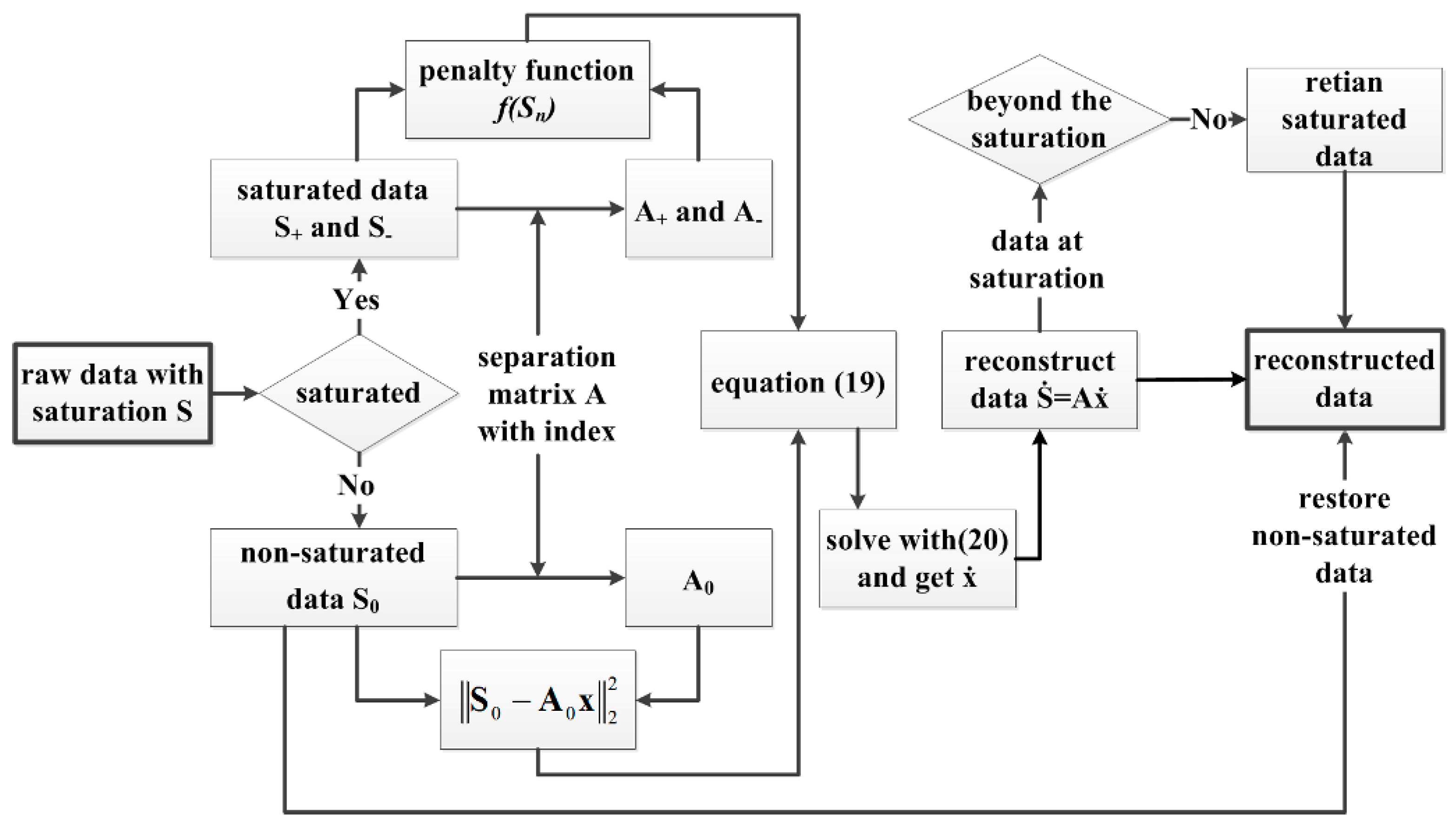
Figure 13.
Workflow of the proposed method.
Figure 13.
Workflow of the proposed method.
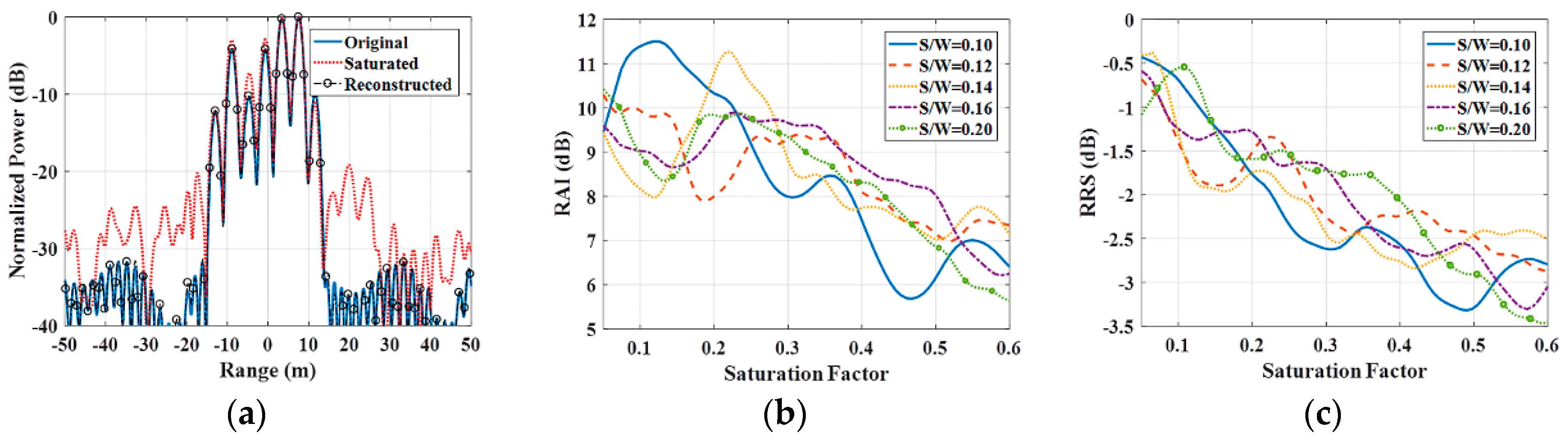
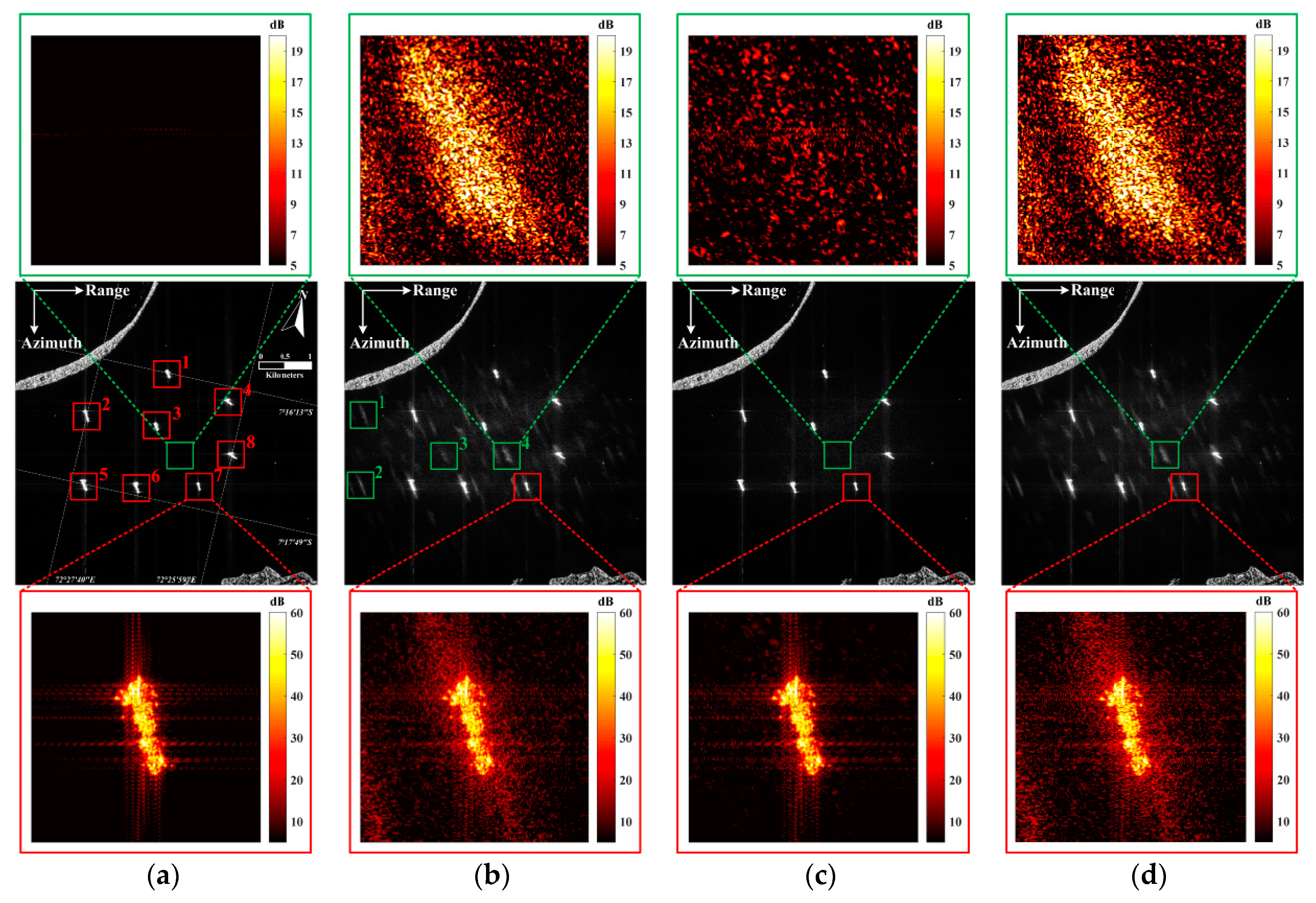
Figure 14.
Performance of the proposed method. The ratio of the intensity of strong targets to that of the background is approximately 30 dB. (a) Pulse compression results with a Hamming window and a 30% saturation factor for the raw data. (b) RAIs for different saturation factors and S/W ratios. (c) RRSs for different saturation factors and S/W ratios. RAI stands for Radiometric Accuracy Improvement. S/W stands for the ratio of the Strong target quantity to the Weak target quantity. RRS stands for Relative value of Reduced Saturation.
Figure 15.
Simulation of 1D pulse compression with a 50% saturation factor. (a) The real part of the raw data. (b) The amplitude of the raw data. (c) The phase of the raw data. (d) Pulse compression results with a Hamming window.
Figure 15.
Simulation of 1D pulse compression with a 50% saturation factor. (a) The real part of the raw data. (b) The amplitude of the raw data. (c) The phase of the raw data. (d) Pulse compression results with a Hamming window.
Figure 16.
Simulation based on real focused data. The original image is from the SLiding spotlight (SL) mode of TerraSAR-X (resolution 1 × 1 m), and the resolution of the simulated image is 3 × 3 m. (a) The non-saturated simulation image. (b) Saturated simulation image, in which there is a series of false targets, with a 9.7% saturated factor. (c) Reconstructed result using the proposed method. (d) Reconstructed result using power loss compensation (PLC factor 1.25).
Figure 17.
Simulation based on real focused data. The original image is from the Ultra-Fine (UF) mode of ALOS-2 (resolution 3 × 3 m), and the resolution of the simulated image is 6 × 6 m. (a) Non-saturated simulation image. (b) Saturated simulation image, in which there is a series of false targets, with a 22% saturated factor. (c) Reconstructed result with proposed method. (d) Reconstructed result using the power loss compensation (PLC factor 1.56).
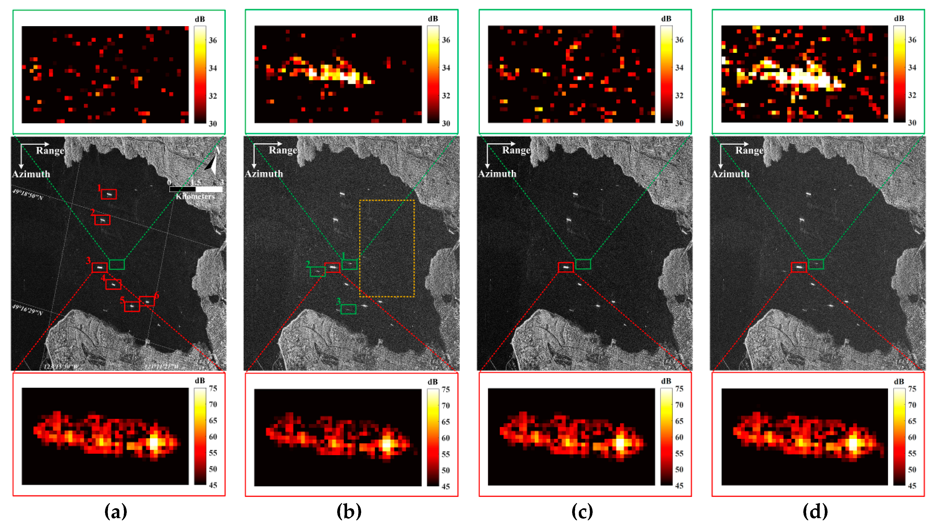
Figure 18.
Simulation based on a real SAR raw data from Radarsat-1. All images were quantized with the same method. (a) Imaging result for the original data. (b) Imaging result for the saturated data with a 25% saturation factor. This image contained a series of false targets beside ships and considerable noise in sea areas. (c) The reconstructed result with the proposed method. (d) The reconstructed result with power loss compensation (PLC factor 1.67).
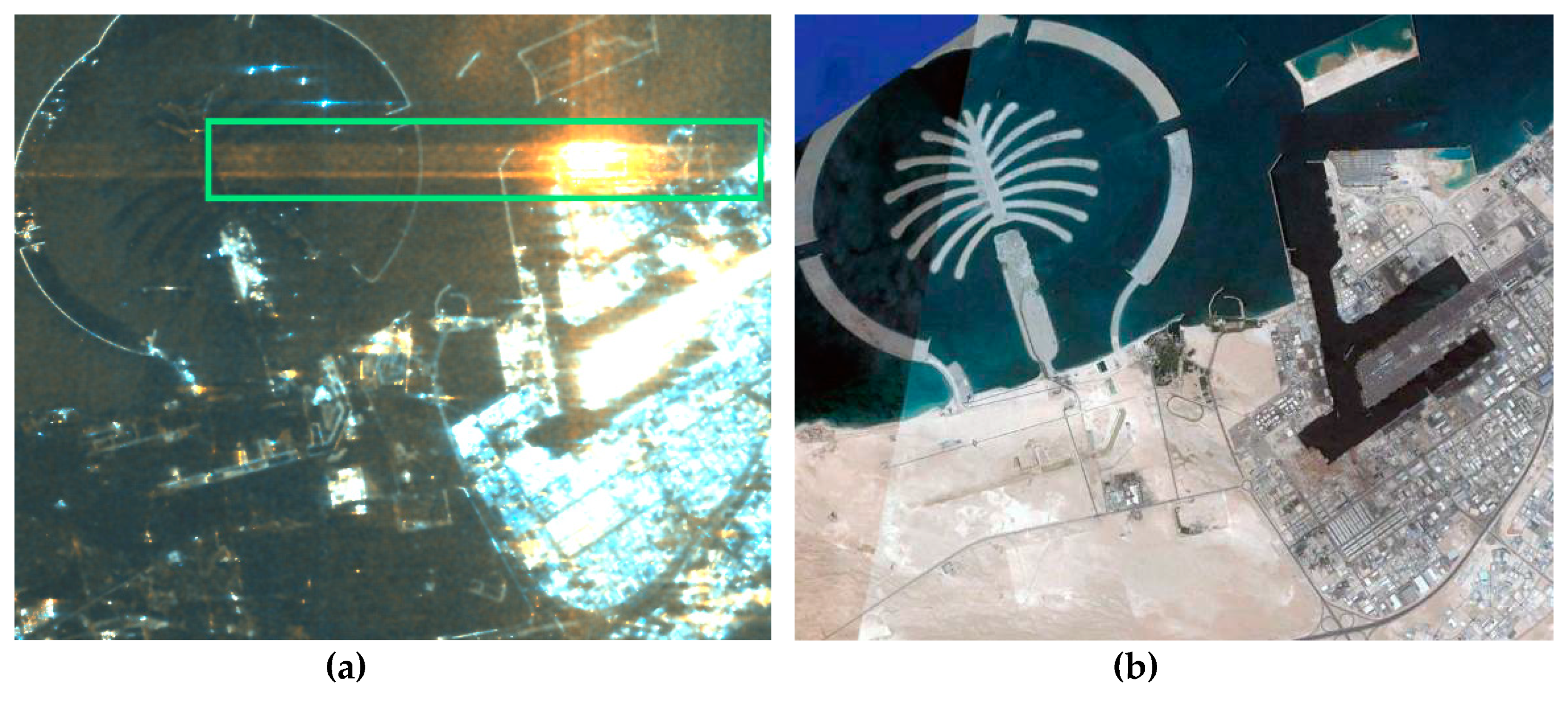
Figure 19.
Polarimetric decomposition mistake caused by ADC saturation. The containers on the top lead to a larger area with orange than the truth. (a) Dual-polarized image from ALOS-1 at Dubai. (Red), (Green), (Blue). (b) Optical image. stands for horizontal-horizontal polarization. stands for horizontal-vertical polarization.
Table 1.
One-dimensional simulation parameters.
Table 1.
One-dimensional simulation parameters.
| Parameter Name | Value | Units |
|---|
| Radar frequency | 9.65 | GHz |
| Bandwidth | 100 | MHz |
| Sampling frequency | 112.6 | MHz |
| Pulse length | 40 | us |
| Saturation factor (clipping factor) | 50% | |
Table 2.
Echo simulation parameters of TerraSAR-X.
Table 2.
Echo simulation parameters of TerraSAR-X.
| Parameter Name | Value | Units |
|---|
| Radar frequency | 9.65 | GHz |
| Bandwidth of pulse | 150 | MHz |
| Sampling frequency | 164.8 | MHz |
| Pulse length | 40 | us |
| Slant range in center | 584 | km |
| Satellite velocity | 7400 | m/s |
| Azimuth bandwidth | 2765 | Hz |
| Pulse repetition frequency | 3451 | Hz |
| Saturation factor (clipping factor) | 9.7% | |
Table 3.
RAIs of the real targets in red boxes.
Table 3.
RAIs of the real targets in red boxes.
| SN 1 | 1 | 2 | 3 | 4 | 5 | 6 | 7 | 8 | Mean |
|---|
| Proposed (dB) | 10.70 | 8.95 | 8.63 | 9.25 | 10.79 | 10.23 | 10.57 | 9.40 | 9.47 dB |
| PLC 2 (dB) | 3.41 | 7.36 | 2.72 | 14.63 | 15.84 | 9.23 | 6.69 | 5.76 | 10.69 dB |
Table 4.
RRSs of the false targets in green boxes.
Table 4.
RRSs of the false targets in green boxes.
| SN | 1 | 2 | 3 | 4 | Mean |
|---|
| Proposed (dB) | 10.39 | 8.62 | 5.49 | 6.46 | 8.16 dB |
| PLC (dB) | −0.43 | −0.43 | −0.43 | −0.43 | −0.43 dB |
Table 5.
Echo simulation parameters of ALOS-2.
Table 5.
Echo simulation parameters of ALOS-2.
| Parameter Name | Value | Units |
|---|
| Radar frequency | 1.24 | GHz |
| Bandwidth of pulse | 38 | MHz |
| Sampling frequency | 52.4 | MHz |
| Pulse length | 25 | us |
| Slant range in center | 703 | km |
| Satellite velocity | 7257 | m/s |
| Azimuth bandwidth | 1671 | Hz |
| Pulse repetition frequency | 2610 | Hz |
| Saturation factor (clipping factor) | 22% | |
Table 6.
RAIs of the real targets in red boxes.
Table 6.
RAIs of the real targets in red boxes.
| SN | 1 | 2 | 3 | 4 | 5 | 6 | Mean |
|---|
| Proposed (dB) | 13.08 | 12.78 | 12.76 | 13.42 | 12.82 | 12.85 | 12.96 dB |
| PLC (dB) | 13.03 | 14.08 | 7.33 | 7.56 | 5.94 | 7.47 | 10.43 dB |
Table 7.
RRSs of the false targets in green boxes.
Table 7.
RRSs of the false targets in green boxes.
| SN | 1 | 2 | 3 | 4 | 5 | Mean |
|---|
| Proposed (dB) | 0.45 | 1.06 | 0.02 | 1.14 | 0.28 | 0.61 dB |
| PLC (dB) | −2.22 | −2.22 | −2.22 | −2.22 | −2.22 | −2.22 dB |
Table 8.
RAIs of the real targets in red boxes.
Table 8.
RAIs of the real targets in red boxes.
| SN | 1 | 2 | 3 | 4 | 5 | 6 | Mean |
|---|
| Proposed (dB) | 8.69 | 9.86 | 11.52 | 8.14 | 8.01 | 7.43 | 9.18 dB |
| PLC (dB) | 8.38 | 2.79 | 5.59 | 8.53 | 8.22 | 5.72 | 6.98 dB |
Table 9.
RRSs of the false targets in green boxes.
Table 9.
RRSs of the false targets in green boxes.
| SN | 1 | 2 | 3 | Mean |
|---|
| Proposed (dB) | 1.32 | 0.20 | 0.05 | 0.56 dB |
| PLC (dB) | −3.08 | −3.08 | −3.08 | −3.08 dB |


