Abstract
Recent studies reported that precipitation and mountain waves induced low tropospheric level circulations may be decoupled or masked by greater spatial scale variability despite generally there is a connection between microphysical processes of precipitation and mountain driven air flows. In this paper we analyse two periods of a winter storm in the Eastern Pyrenees mountain range (NE Spain) with different mountain wave induced circulations and low-level turbulence as revealed by Micro Rain Radar (MRR), microwave radiometer and Parsivel disdrometer data during the Cerdanya-2017 field campaign. We find that during the event studied mountain wave wind circulations and low-level turbulence do not affect neither the snow crystal riming or aggregation along the vertical column nor the surface particle size distribution of the snow. This study illustrates that precipitation profiles and mountain induced circulations may be decoupled which can be very relevant for either ground-based or spaceborne remote sensing of precipitation.
Keywords:
MRR; Parsivel disdrometer; orographic precipitation; mountain waves; rotor; winter storm; Pyrenees 1. Introduction
Mountains are a major factor in precipitation modification at local and global scales [1]. As clouds interact with mountains, subsequent precipitation patterns may be deeply influenced by the terrain variability. Local-scale mountain circulations have evidenced to influence the microphysical processes that determine the precipitation particle size distribution (PSD) reaching the ground. For example, examining field observations from the MAP [2] and IMPROVE [3] campaigns it has been found that stable baroclinic systems passing over mountains frequently produce a vertical wind shear layer over the windward slope of the mountain [4]. Using radar observations, it has been observed that the turbulence and small updraughts produced inside the shear layer enhance ice riming and raindrop coalescence that contributes to the growth of precipitation particles [5,6]. Combining radar observations and model simulations it has been found that mountain waves can modulate the precipitation patterns of the winter storms [7,8]. However, during a winter observational campaign, Kingsmill et al. [9] observed a vertically propagating mountain wave forced by the Park Range (northern Colorado) using an airborne vertically pointing W-band (95GHz) Doppler radar. They studied 10-minutely spaced cross-sections across the barrier and did not found evidence of impact of the mountain-wave induced circulations in the precipitation patterns. Their results suggested that, due to the complex nature of the dynamical and microphysical processes involved in which many scales might be interacting, it would be necessary to employ different types of observations to further analyse this apparent disconnection between mountain-wave induced circulations and precipitation processes.
To address this issue, in this paper we study the relation between orographic precipitation and leeward vertically propagating motions forced by the Pyrenees mountain range at different temporal scales from minutes to hours using a vertically pointing Micro Rain Radar, a Parsivel laser disdrometer and other instrumentation set in the Cerdanya-2017 (C2017) field campaign [10,11]. Our initial hypothesis is that mountain wave induced circulations modify precipitation features when large scale variability of the precipitation does not hamper the identification of small-scale interactions. Instrumentation used in the study is briefly described in Section 2. Results are described in Section 3: In Section 3.1 and Section 3.2 we describe the snowfall event analysed showing how the large-scale variability is the main source of PSD fluctuations. To isolate the mountain induced atmospheric circulations and associated kinematic structures, two periods with minor variability among them are selected and analysed in Section 3.3. The conclusions obtained are drawn in Section 4.
2. Data and Methods
2.1. Rain Gauges
Solid precipitation for the region of study was measured by the C2017 field campaign automatic weather station network (AWS), consisting in a selection of the AWS of the four different rain gauge networks managed by the Spanish Meteorological Service (AEMET), the Meteorological Service of Catalonia (SMC), the Snow and Mountain Research Centre of Andorra (CENMA) and an ad-hoc network provided by the French Meteorological Service (Météo-France). As it is well known, AWS tend to underestimate solid precipitation, especially when the wind is strong [12,13]. Precipitation amounts presented in Figure 1 have been corrected using the transference functions considering wind and precipitation records developed by Buisan et al. [14] for tipping-bucket gauges and by Kochendorfer et al. [15] for single-Alter-shielded weighting gauges.
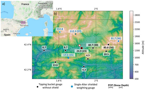
Figure 1.
(a) Location of the study area and (b) accumulated precipitation (PCP) [mm] and snow depth increment [cm] (in parentheses, if available) from 15 to 16 January 2017, showing the locations of single-Alter shielded weighting gauges (blue solid circles), tipping bucket heated gauges (black solid circles), Das station where the Micro Rain Radar (MRR) and the Parsivel disdrometer were located (back circle with red contour), the location of Malniu station (blue circle with orange contour) and the location of the UHF wind profiler (white circle with red contour). Precipitation amounts are corrected for undercatch wind effects (see text for details).
2.2. Micro Rain Radar
A Micro Rain Radar (model MRR-2), a compact FM-CW (Frequency-Modulated Continuous-Wave) Doppler radar that operates at 24 GHz (K-band), was employed in this study [16]. The radar uses an offset antenna with a vertical beam orientation to scan a vertical profile every 10 seconds. Although MRR was first developed to observe liquid precipitation and has been widely used for this purpose (see for example [17,18,19]), its application to snow observation has also been demonstrated [20] despite solid precipitation particle preferential orientations and aspect ratios influence radar reflectivity estimates posing additional challenges compared to liquid precipitation [21]. MRR has been recently applied to solid precipitation studies to analyse snow band microphysics for US east coast winter storms [22], lake-effect convection at Lake Ontario [23], radar reflectivity vs snowfall rate relationships over Antarctica [24], Antarctic ice mass balance [25], precipitation decrease due the katabatic winds [26] and verification of spaceborne snowfall estimates from the CLOUDSAT satellite [27].
In this study MRR data was recorded with 100 m vertical resolution up to 3 km above ground level, integrating measurements every 60 seconds and applying the post-processing methodology proposed by Maahn and Kollias [28] which is especially suited for snowfall observations and provides reliable values of equivalent reflectivity, Doppler velocity and spectral width.
2.3. Parsivel Disdrometer
Particle Size Velocity (Parsivel) is an optical disdrometer whose measurements are based on the attenuation of a laser beam obscured by falling precipitation particles. From the reduction of the output voltage and the signal duration, Parsivel determines the particle size and velocity respectively. In this study an OTT Parsivel disdrometer [29] with 1-minute data average was used.
Parsivel assumes that precipitation particles are spheroids, which is a good approximation for small and medium sized raindrops. However, this assumption largely departs from the reality for solid hydrometeors such as snowflakes. Nonetheless Battaglia et al. [30] showed that Parsivel data can be adapted to measure snow precipitation events by calculating the widest horizontal dimension (WHD) to characterize snowflake size (see Appendix A for further details). This is the only size parameter that can be retrieved from Parsivel solid precipitation data, although according to Battaglia et al. [30] it has no direct microphysical meaning. WHD estimates have large uncertainties for small particles: Ref. [30] reported a mean underestimation of around 20% for small particles.
The equivalent radar reflectivity factor (Ze) can also be retrieved from Parsivel snow observations using the algorithm developed by Löffler-Mang and Blahak [31] considering that, due to the different dielectric properties of solid precipitation particles, some correction factors should be applied [32]. The method requires to assume a single crystal mass-size relation to perform the calculations. We considered the study of Locatelli and Hobbs [33] which determined empirical mass-size relations for 14 solid precipitation types and applied them to compare the Ze between the disdrometer data and the third lowest bin (300 m above ground level, agl) MRR processed data. Details of this analysis are described in Appendix B—see the scatter plots of Figure A1 and Table A1. According to this analysis two solid precipitation unrimed particles (types so-called aud and ausp, described in Table A1) matched much better our data set than the others for the event studied.
3. Results
3.1. General Description of the 15–16 January Event
On 15 and 16 January 2017 a major blizzard event occurred in the Pyrenees (NE Spain) bringing extreme low temperatures, heavy snowfall and gale-force winds. The episode occurred as a consequence of a strong northern flow under a north-to-south oriented jet and the presence of symmetric instability and an atmospheric river that impinged directly to the Pyrenees, as illustrated by ERA-Interim 0.75° × 0.75° resolution reanalysis data [34]—see geopotential height fields at 850 and 500 hPa and 850 hPa equivalent temperature, and streamlines and specific humidity at 700 hPa (Figure 2a,b). These synoptic conditions remained almost stationary for 36 h until the afternoon of 16 January when moist air was replaced by dry air coming from central Europe. As reported in previous studies, intense meridional flow impinging perpendicularly to the Pyrenees mountain range is a classic characteristic of both warm season [35,36] and cold season [37] heavy precipitation events due to orographic effects. Figure 1b displays the precipitation amounts and snowfall depth accumulations recorded by the field campaign network and the location of the Cerdanya valley.
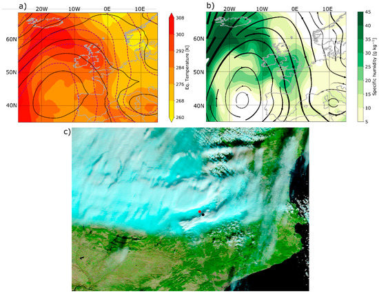
Figure 2.
Upper panels display ERA-Interim reanalysis data for 15 Jan 2017 12 UTC showing: (a) Geopotential height [gpm] at 850 hPa and 500 hPa (black solid lines and purple dashed lines respectively) and equivalent temperature at 850 hPa (shaded colours); and (b) streamlines (line width proportional to the wind speed) and specific humidity at 700 hPa (yellow-green shaded colours). (c) MODIS corrected reflectance in false colour (Bands 7-2-1) measured by the Terra satellite on 15 Jan 2017 10:35 UTC. Black and Red dots indicate respectively the position of the MRR and the UHF wind-profiler.
The sounding launched at Das at 10:35 UTC indicates that this event occurred under moist-neutral stratification as can be seen in the well mixed layer extending from 800 to 680 hPa capped by a strong inversion (Figure 3). The 12:00 UTC sounding at Bordeaux (located about 300 km north-west from the area of study) confirms that similar conditions held upstream (not shown). This sounding indicates a stable flow impinging to the mountain range with a moist Brunt-Väisälä frequency of about 10−2 s−1 and a moist Froude number about 0.6. These conditions and the inversion over the mountain top were favourable for the development of both trapped lee waves and vertically propagating mountain waves that can be inferred from the satellite imagery shown in Figure 2c. A preliminary analysis of the event by Udina et al. [38] showed that the wavelength of the wave present in the morning shortened in the afternoon favouring the appearance of a rotor.
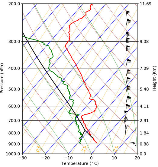
Figure 3.
Atmospheric sounding at Das launched on 15 Jan 2017 at 12:37 UTC.
3.2. Evolution of the 15–16 January Event
This winter storm was intensively observed during the C2017 field campaign [38] and generated mountain waves at the leeside of the Pyrenees, a common feature observed at this area [39]. The main observatory was located at Das and besides an AWS, an MRR, and a Parsivel disdrometer described in the previous section, it also included additional instrumentation such as a multichannel microwave radiometer, a ceilometer and a UHF wind profiler. Das is located at 1100 m above sea level (asl), leeward of the main mountain range (maximum heights about 2900 m asl) but surrounded by a secondary mountain range (maximum heights about 2500 m asl) in the opposite direction (see Figure 1).
The evolution of the snowfall event over Das observatory is displayed in Figure 4, showing MRR reflectivity and Parsivel derived reflectivity (Figure 4a), MRR spectral width and Doppler velocity (Figure 4b,c respectively), UHF vertical and horizontal velocity (Figure 4d) and Parsivel PSD (Figure 4e). During the event three main stages regarding the precipitation (reflectivity and PSD) can be distinguished:
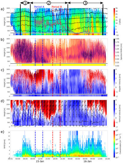
Figure 4.
(a) Radar reflectivity [dBZ] from MRR (above black line) and Parsivel (below black line), the latter calculated assuming snow aggregates of unrimed dendrites or dendrites (see text). (b) Spectral Width [ms−1] from MRR (above black line) and Parsivel derived type of precipitation—where snow and sleet are indicated by yellow and black colours, respectively. (c) Particle Doppler fall velocity [ms−1] from MRR (above black line) and Parsivel measured particle fall velocity (below black line). (d) Inverted vertical velocity [ms−1] and horizontal wind speed and direction [wind barbs in ms−1] from UHF wind-profiler. (e) Parsivel particle concentration as a function of the widest hydrometeor diameter [m−3m−1]. Vertical black lines in (a) indicate the three stages discussed in the text. Vertical blue and red dashed lines indicate the mountain wave period (Period A) and the rotor period (Period B), respectively. Dotted black lines and the grey points in (a) indicate microwave radiometer derived isotherm levels and cloud base height, respectively.
- Stage 1: From 5:00 to 8:00 UTC on 15 January, some snow showers with reflectivity in pockets were observed over Das. During this stage precipitation particles measured by the Parsivel disdrometer were very large as expected from aggregation inside the reflectivity pockets, similarly as in the study reported by [40].
- Stage 2: From 8:00 UTC to 23:00 UTC on 15 January, MRR and Parsivel reflectivity scaled back and precipitation resembled to be more constant and lighter. Particles arriving to the ground were mostly small (WHD < 3 mm).
- Stage 3: From 15 January 23:00 UTC to 16 January 13:00 UTC, reflectivity was again enhanced increasing the temporal variability due to new snow showers. During this stage, the largest precipitation particles of the event were observed while small particles also increased in number.
Local scale mountain induced circulations can be inferred from MRR thanks to the ability of snowflakes to trace the vertical movements and the turbulence of the air [41], despite MRR estimates are based on the backscattering of precipitation particles and not in air movement as it is the case, for example, of a UHF wind-profiler. Hence, MRR spectral width and Doppler fall speed profiles, for the specific case of snow observations, can be used as a proxy of the vertical movements and turbulence over the MRR location, respectively. We separate below the analysis of the evolution of vertical velocity and spectral width.
- Doppler velocity is dominated by updrafts beyond 1500 m agl over the MRR until 15:00 UTC, revealing the location of the upstream part of a mountain wave that it is consistent with the measures of the UHF wind profiler located 3 km northwest of Das. After that, updrafts steadily reduce and fall velocities dominate over the MRR location. This regime change has been identified as a mountain wave, diminishing its wavelength around 15:00 UTC and generating a rotor later [38]. The returning current of the rotor was observed by the MRR as 5 ms−1 northward flow at low levels (see Period B in Figure 4d). Falling velocities in upper MRR levels dominate until approximately 5:00 UTC on 16 January with the appearance of new updrafts that may be associated to a new mountain wave and may extend to the low levels during the largest convective cells.
- During Stage 1, large values of spectral width dominate at all height levels. When the towering reflectivity enhancement ceases, spectral width over 2000 m above ground level dramatically decreases, but high values still dominate at low levels. At 16:00 UTC, coinciding with a sudden surface temperature diminution and wind direction change (Figure 5), spectral width drops-off at low-levels, presumably due to a nocturnal cold pool formation. From this moment to 4:00 UTC, three decoupled layers are observed even when reflectivity pockets start again. After 4:00 UTC spectral width gets enhanced again at middle and upper levels, but the low-level layer remains decoupled. This behaviour is qualitatively consistent with the evolution of Turbulence Kinetic Energy derived from UHF wind-profiler data for the same period (not shown).
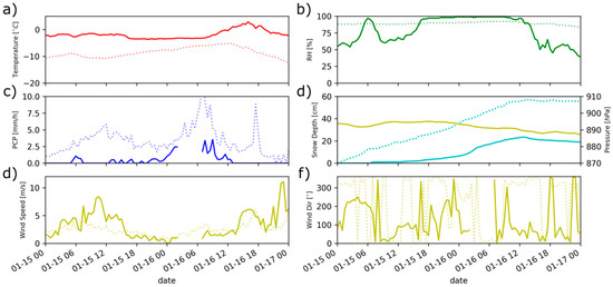 Figure 5. Automatic weather station network (AWS) observations from Das (solid line) and Malniu (dotted line) of (a) temperature, (b) relative humidity, (c) precipitation rate, (d) snow depth (blue lines) and surface pressure (in Das only; yellow line), (e) wind speed and (f) wind direction. Dates are indicated considering the format MM-DD HH (month-day hour) in UTC.
The evolution of this event illustrates that precipitation processes present transient features dominated by deeper tropospheric processes unrelated with the mountain kinematic structures associated with induced circulations. Comparing MRR reflectivity, Doppler velocity and spectral width, we do not observe a simple relationship between the precipitation variability and changes in the vertical velocity or turbulence, highlighting the great complexity of the underlying processes. Nonetheless, as stated in the study carried out by Kingsmill et al. [9], we cannot draw a definite conclusion from these observations, since small scale circulation variability might be masked by greater spatial scale variability.
3.3. Impact of Local Kinematic Structures into Precipitation Patterns
We have seen that the main sources of precipitation variability are transient processes driven by synoptic or mesoscale variations. But what is the role of the small-scale circulations such as waves and rotors induced by mountains? To answer this question, we closely analysed two 3-hour periods with the same precipitation structure in the Stage 2 but with different mountain induced circulations. The first period selected (Period A) is comprised between 10:00 UTC and 13:00 UTC when the mountain wave was wide enough to produce updrafts over the MRR. The second period selected (Period B) ranges from 17:00 to 20:00 UTC and is characterized by the presence of a rotor, with the MRR located at its descending branch. As it can be seen in Figure 4, wind vertical movements and turbulence illustrated by MRR and UHF wind-profiler vertical velocity and MRR spectral width prove to be very different. Comparing the precipitation patterns of both periods, illustrated by MRR reflectivity and Parsivel PSD, more similarities can be noted. During Period B reflectivity slightly decreases with respect to Period A but PSD at ground level looks fairly constant. It is worth to mention that during Period A the cloud base remains relatively constant (ca. 1300 m agl), but it raises and shows sharp variations during Period B.
3.3.1. MRR Observations
To assess how the change in the mountain-wave induced circulations affects the distribution of the precipitation in the vertical, Figure 6 shows the MRR reflectivity, velocity and spectral width spectrogram of both periods; mean cloud base and temperature levels from microwave radiometer estimates are also indicated in the plots. Spectral width and vertical velocity show large variations between both periods.
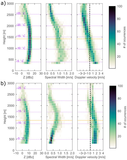
Figure 6.
MRR reflectivity [dBZ], spectral width [m/s] and Doppler velocity [m/s] spectrogram for (a) Period A and (b) Period B. Dotted lines indicate average isotherm heights (purple lines) and average cloud base heights (orange lines) derived from microwave radiometer and ceilometer data respectively.
- During Period A, spectral width shows large values between 1.0 and 1.5 m s−1 at low levels, values around 1.0 m s−1 between 1000 and 2000 m agl, and values lower than 1.0 m s−1 above 2000 m agl. Vertical velocity shows a gradient from downward velocities around 2 m s−1 to upward velocities around -2 m s−1 that are the result of overlaying the vertical movements of the wind with the falling velocity of the particles with respect to the air—typical snowflakes terminal velocities are about 1 m s−1 [42] but they may fluctuate from the mean [43].
- During Period B, three decoupled layers can be distinguished: the bottom and the top layer with very low turbulence, under 0.5 m s−1, and a middle shear layer [4] with large turbulence between 0.5 and 1.0 m s−1. Fall velocities between 0 and 2 m s−1 dominate in this period at all levels. It is observed a slight increase of the fall velocity closer to the ground inside the shear layer.
Both periods show similar features regarding the reflectivity: an increase from 3000 m to 2000 m agl where the snow crystals may be growing downward, a band with reflectivity values stabilized and finally a reflectivity decrease at low levels that may be related to the snow sublimation downwind of the mountain [42]. The main difference in the MRR reflectivity between both periods is the magnitude, that is 5 dBZ greater in all the profile during Period A compared with Period B, but as stated the structure is similar. Snow growing for both periods is located aloft the −15 °C isotherm level suggesting that crystal formation is outside the dendrite growing zone [44]. It has been observed that dendrites are more sensible to aggregation due to mechanical entanglement [45], so the lack of increasing reflectivity with decreasing height below the −15 °C isotherm suggests the absence of dendrite aggregation. The comparison of MRR reflectivity and spectral width does not indicate a clear association between downward snow growth and turbulence during this part of the event.
3.3.2. Parsivel Observations
Figure 7a shows the averaged PSD of the two 3-hour periods (bold dashed lines) recorded by the Parsivel disdrometer. It is evident that both periods show a similar particle size distribution that confirms the similar reflectivity at low levels observed by the MRR. To visualize the variability and verify that the similarity is not a coincidence due to temporal averaging, we also plotted the three averaged 1-hour segments for both mountain wave and rotor periods. Although the variability is larger for small particles (less than 1 mm), specially for Period B, it is shown that the distribution of most particle sizes between 1 and 3 mm follow the same potential scaling. Additional confirmation is provided by Figure 8 which shows that PSD in this stage is totally different from other stages of the case study.
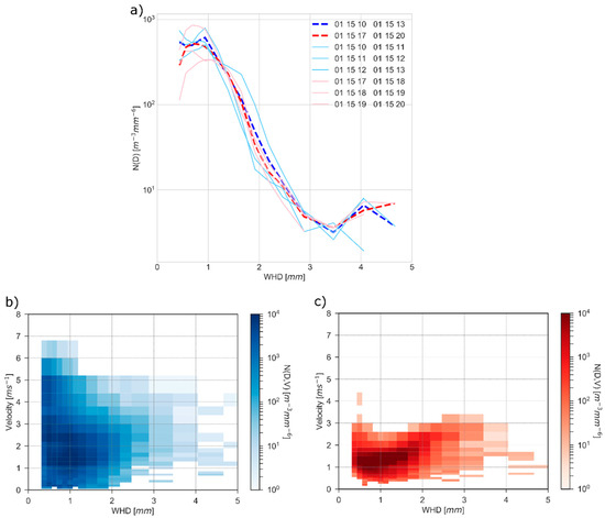
Figure 7.
(a) Particle Size Distribution averaged for the time interval measured by Parsivel for mountain wave period (Period A, in blues) and rotor period (Period B, in reds). (b,c) Particle size and velocity distribution for (b) Period A and (c) Period B. Dates are indicated considering the format MM-DD HH (month-day hour) in UTC.
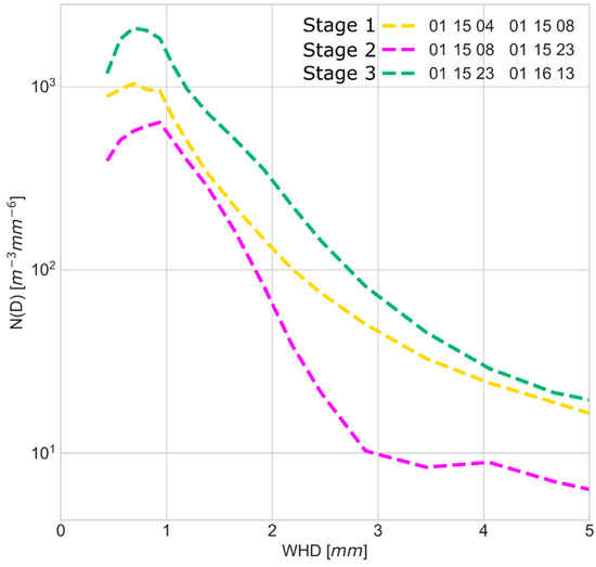
Figure 8.
Hydrometeor Particle Size Distribution N(D) measured by Parsivel disdrometer for the three different storm stages studied. Dates are indicated considering the format MM-DD HH (month-day hour) in UTC.
We also compared the full spectra of velocities and diameters of the two periods in Figure 7b,c. Interestingly, despite both periods have an identical PSD, the spectra of velocities measured by Parsivel are substantially different. Period A shows a broader spectrum of velocities, from 0.0 to 6.5 m s−1 for small particles, than in Period B, when values range approximately from 0.5 to 2.5 m s−1 for all particles. This difference may be explained by the enhanced near-ground turbulence during Period A that removes any sensitivity of the snow particles to the terminal velocity [46] and the decrease of turbulence during Period B, which is probably more associated to the diurnal regime than to the mountain kinematic structures. It is worth to note that, as observed in Figure 7, the broader spectrum of particle velocities does not lead to downward snow growing neither by particle aggregation nor riming as it would be expected due to the small-scale updraughts and downdraughts inside the turbulent boundary layer [5,6,40,42].
4. Discussion and Conclusions
During the 15 and 16 January 2017, a major snowfall event was observed using remote sensing instruments in the Cerdanya valley at the Pyrenees mountain massif (NE Spain). In this study, we analysed two periods with the same synoptic and mesoscale features but with different local scale circulations induced by mountain wave changes. As evidenced by ground-based Parsivel observations, changes in mountain-wave kinematic structures had a minimum effect over the PSD observed leeside of the Pyrenees during the Stage 2 of this winter storm, when the precipitation conditions remained stationary. Nonetheless, they affected the fall velocity distribution of the particles near the ground. Unexpectedly, the broader range of particle velocities due the overturning cells did not imply a greater aggregation or crystal modification as suggested by Parsivel-MRR comparisons. The relatively cold continental environment of the Cerdanya valley, isolated from maritime influences, may explain the absence of riming which is more prone to occur over coastal mountains due to the increased liquid water inside the winter clouds [6,40,47]. In this case, liquid water carried by the atmospheric river could have been depleted on the windward side of the mountain range. The apparent lack of aggregation may be explained by the lack of dendritic growth, so the particles grown aloft probably fall pristine through the turbulent layer without experiencing mechanical aggregation during their path, as described in [45]. The low-level sublimation may also contribute to obtain identical PSD in both periods.
Our results agree and complete those of Kingsmill et al. [9] who did not find evidence of mountain modification of precipitation profiles in Park Range, Colorado during field measurements. Kingsmill et al. [9] argued that large scale variability may hide small mountain interactions. As the two periods analysed had minor variability among them, our results suggest that in this case study kinematic structures generated as a result of mountain wave induced circulations as gravity waves, rotors and changes in turbulence did not modify the precipitation particle distribution at low levels and did not contribute to a larger aggregation. We speculate that the conditions that cause the decoupling and the lack of sensitivity of the snow crystals to the turbulence are (1) a cold continental environment with low liquid water content which would suppress the growth by riming and (2) lack of dendritic form which would reduce the growth by aggregation, leaving only the possibility of depositional growth. Our habit type analysis suggests the lack of riming, but to test this hypothesis it would be necessary further observations of liquid water content and ice concentration that unfortunately were not available for this experimental campaign. However, these conditions would be consistent with the results of Aikins et al. [40] who observed snow growth by aggregation (instead of riming observed at coastal mountains) favoured by the turbulence near the dendritic growth zone which is absent in our event.
Recent results from the SNOWIE field campaign about winter orographic clouds and precipitation [48] found a frequent decoupling between the orographic cloud layer where precipitation was formed and the near-surface air layer, which was trapped at the bottom of the valley. In our study, we also find a decoupling between ground-level conditions and higher levels but affecting precipitation profiles as well. These results illustrate the high variability of winter precipitation profiles in complex terrain and contribute to improve our understanding of discrepancies between surface precipitation and ground-based or spaceborne remote sensing estimates based on measurements performed above ground level over the so-called blind zone [49]. This is particularly relevant for recent studies using CloudSat or GPM core satellite data [50,51,52].
Author Contributions
Conceptualization and investigation, S.G.; data curation, S.G., J.B., M.U., B.C., A.P., and L.T.; Writing—Original Draft preparation, S.G.; Writing—Review and Editing, J.B., M.U., B.C., A.P., and L.T.; supervision, J.B.
Funding
The Cerdanya-2017 field campaign is a research effort organized by the University of the Balearic Islands, the University of Barcelona, METEO-FRANCE and the Meteorological Service of Catalonia and was funded by the Spanish projects CGL2015-65627-C3-1-R (MINECO/FEDER), CGL2015-65627-C3-2-R (MINECO/FEDER), CGL2016-81828-REDT (MINECO) and the Water Research Institute (IdRA) of the University of Barcelona. Research activities of S.G. and of J.B., M.U., B.C., are supported respectively by the ANTALP (Antarctic, Arctic and Alpine Environments, 2017-SGR-1102) and the Meteorology (2017-SGR- 0651) Research Groups of the Catalan Government.
Acknowledgments
This work was performed under the framework of the Hydrological Mediterranean Experiment (HyMeX) programme. We thank the METEO-FRANCE/CNRM/GMEI/LISA, 4M and TRAMM teams for their contribution to the data acquisition and treatment. ERA interim data was downloaded from the European Centre for Medium-Range Weather Forecasts (ECMWF) Data Server. We thank the three anonymous reviewers for their insights that helped to improve this manuscript.
Conflicts of Interest
The authors declare no conflict of interest.
Appendix A
The precipitation particle Widest Horizontal Dimension (WHD) was calculated using the algorithm developed by Battaglia et al. [30]. WHD is defined as
where Deq is the equivalent sphere diameter of the particle measured by Parsivel and ar is the axial ratio of the spheroid that is assumed to vary from 0.7 to 1.0 according the following expression:
Appendix B
To analyse which type of solid precipitation particle matched best our data we compared the equivalent radar reflectivity factor (Ze) retrieved from Parsivel with the third lowest MRR bin, the first usable bin according to Maahn and Kollias [28].
To retrieve the Parsivel Ze we used the algorithm developed by Löffler-Mang and Blahak [31], so Ze was calculated following Smith [32]:
where CK is the complex refraction index for ice (0.195), ni are the number of measured precipitation particles in a class i with a mean diameter Di and mean velocity vi during measuring time t (set to 60s), F is the measuring area, and CM,i is a correction factor that takes into account of the mass-size relation m = a D b of the ice crystal calculated by Locatelly and Hobbs [33] and it is calculated using the following formula:
where = 0.92 kg m−3 is the density of ice, and mk and Dk are the mass and the diameter of a particle k.
Figure A1 provides a comparison between MRR Ze observed and the Parsivel Ze calculated to analyse which type of crystal matched better our data using a linear regression:
We expect that a perfect match would be MRR_Ze = Parsivel_Ze, i.e., b = 1 and a = 0. Therefore, as b approaches to 1, more likely this crystal type matches the observations. However, a is more difficult to evaluate because we are not comparing the reflectivity at the same heights and it is difficult to correct MRR Ze to the ground because instead of growing downwards it is decreasing, as shown in Figure 6.

Figure A1.
Linear regressions between reflectivity observed by MRR and calculated by Parsivel using 14 different mass-size empirical relations of crystals. Dashed black line indicates the 1:1 relation.

Table A1.
Linear regression (parameters a, b of MRR_Ze= a + b · Parsivel_Ze and correlation coefficient r) of reflectivity Ze calculated using the third lowest MRR bin (300 m) and Parsivel data using different mass-size empirical relations of crystals according to Locatelli and Hobbs [33]. Columns correspond to the whole event (All), and Stages 1, 2 and 3 (see Figure 4).
| All | 1 | 2 | 3 | |||||
|---|---|---|---|---|---|---|---|---|
| Solid Precipitation Particle Type | b | a | b | A | b | a | b | a |
| Aggregates of unrimed side planes (ausp) | 0.657 | 9.29 | 0.430 | 12.17 | 0.777 | 7.05 | 0.630 | 10.62 |
| Aggregates of unrimed assemblages of plates, side planes, bullets and columns (aup) | 0.555 | 8.14 | 0.375 | 11.08 | 0.672 | 6.33 | 0.438 | 10.49 |
| Aggregates of densely rimed assemblages of dendrites or dendrites (arp) | 0.555 | 8.14 | 0.375 | 11.08 | 0.672 | 6.33 | 0.438 | 10.49 |
| Aggregates of unrimed assemblages of dendrites or dendrites (aud) | 0.657 | 5.86 | 0.430 | 9.93 | 0.777 | 2.99 | 0.630 | 7.33 |
| Densely rimed assemblages of dendrites (dra) | 0.513 | 7.34 | 0.353 | 10.40 | 0.618 | 5.56 | 0.374 | 10.31 |
| Densely rimed dendrites (drd) | 0.473 | 10.78 | 0.331 | 12.69 | 0.562 | 9.82 | 0.321 | 13.04 |
| Densely rimed columns (drc) | 0.473 | 7.55 | 0.331 | 10.42 | 0.562 | 5.97 | 0.321 | 10.84 |
| Lump graupel 3 (lg3) | 0.403 | 1.58 | 0.291 | 5.89 | 0.457 | −0.56 | 0.245 | 7.80 |
| Lump graupel 2 (lg2) | 0.389 | 3.55 | 0.283 | 7.25 | 0.434 | 1.78 | 0.230 | 9.16 |
| Lump graupel 1 (lg1) | 0.361 | 5.34 | 0.266 | 8.45 | 0.391 | 3.93 | 0.206 | 10.46 |
| Graupel-like snow lump type (gl) | 0.513 | 5.50 | 0.353 | 9.14 | 0.618 | 3.34 | 0.374 | 8.97 |
| Graupel-like snow hexagonal type (gh) | 0.454 | 9.08 | 0.320 | 11.44 | 0.534 | 7.85 | 0.299 | 12.02 |
| Conical graupel (cg) | 0.420 | 3.96 | 0.301 | 7.68 | 0.482 | 2.03 | 0.261 | 9.06 |
| Hexagonal graupel (hg) | 0.374 | 5.33 | 0.274 | 8.50 | 0.411 | 3.85 | 0.217 | 10.34 |
References
- Houze, R.A. Orographic effects on precipitating clouds. Rev. Geophys. 2012, 50, RG1001. [Google Scholar] [CrossRef]
- Bougeault, P.; Binder, P.; Buzzi, A.; Dirks, R.; Houze, R.; Kuettner, J.; Smith, R.B.; Steinacker, R.; Volkert, H. The MAP Special Observing Period. Bull. Am. Meteorol. Soc. 2001, 82, 433–462. [Google Scholar]
- Stoelinga, M.T.; Hobbs, P.V.; Mass, C.F.; Locatelli, J.D.; Colle, B.A.; Houze, R.A.; Rangno, A.L.; Bond, N.A.; Smull, B.F.; Rasmussen, R.M.; et al. Improvement of microphysical parameterization through observational verification experiment. Bull. Am. Meteorol. Soc. 2003, 84, 1807–1826. [Google Scholar] [CrossRef]
- Medina, S.; Smull, B.F.; Houze, R.A.; Steiner, M. Cross-Barrier Flow during Orographic Precipitation Events: Results from MAP and IMPROVE. J. Atmos. Sci. 2005, 62, 3580–3598. [Google Scholar] [CrossRef][Green Version]
- Yuter, S.E.; Houze, R.A. Microphysical modes of precipitation growth determined by S-band vertically pointing radar in orographic precipitation during MAP. Q. J. R. Meteorol. Soc. 2003, 129, 455–476. [Google Scholar] [CrossRef]
- Houze, R.A.; Medina, S. Turbulence as a Mechanism for Orographic Precipitation Enhancement. J. Atmos. Sci. 2005, 62, 3599–3623. [Google Scholar]
- Garvert, M.F.; Smull, B.; Mass, C. Multiscale Mountain Waves Influencing a Major Orographic Precipitation Event. J. Atmos. Sci. 2007, 64, 711–737. [Google Scholar] [CrossRef]
- Tsai, C.-L.; Kim, K.; Liou, Y.-C.; Lee, G.; Yu, C.-K. Impacts of Topography on Airflow and Precipitation in the Pyeongchang Area Seen from Multiple-Doppler Radar Observations. Mon. Weather Rev. 2018, 146, 3401–3424. [Google Scholar]
- Kingsmill, D.E.; Persson, P.O.G.; Haimov, S.; Shupe, M.D. Mountain waves and orographic precipitation in a northern Colorado winter storm. Q. J. R. Meteorol. Soc. 2016, 142, 836–853. [Google Scholar] [CrossRef]
- Cuixart, J.; Conangla, L.; Martínez-Villagrasa, D.; Wrenger, B.; Miró, J.R.; Simó, G.; Jiménez, M.A. Evolution of the temperature profile during the life-cycle of a valley-confined cold pool in the Pyrenees. In Proceedings of the 34th International Conference on Alpine Meteorology, Reykjavík, Iceland, 18–23 June 2017; pp. 191–192. [Google Scholar]
- Paci, A.; Cuixart, J.; Bech, J.; Soler, M.R.; Miró, J.R.; Aressy, P.; Arús, J.; Barrié, J.; Bouhours, G.; Bravo, M.; et al. The Cerdanya-2017 field experiment: An overview of the campaign and a few preliminary results. In Proceedings of the 34th International Conference on Alpine Meteorology, Reykjavík, Iceland, 18–23 June 2017; pp. 169–170. [Google Scholar]
- Rasmussen, R.; Baker, B.; Kochendorfer, J.; Meyers, T.; Landolt, S.; Fischer, A.P.; Black, J.; Thériault, J.M.; Kucera, P.; Gochis, D.; et al. How well are we measuring snow: The NOAA/FAA/NCAR winter precipitation test bed. Bull. Am. Meteorol. Soc. 2012, 93, 811–829. [Google Scholar] [CrossRef]
- Kochendorfer, J.; Rasmussen, R.; Wolff, M.; Baker, B.; Hall, M.E.; Meyers, T.; Landolt, S.; Jachcik, A.; Isaksen, K.; Brækkan, R.; et al. The quantification and correction of wind-induced precipitation measurement errors. Hydrol. Earth Syst. Sci. 2017, 21, 1973–1989. [Google Scholar] [CrossRef]
- Buisán, S.T.; Earle, M.E.; Collado, J.L.; Kochendorfer, J.; Alastrué, J.; Wolff, M.; Smith, C.D.; López-Moreno, J.I. Assessment of snowfall accumulation underestimation by tipping bucket gauges in the Spanish operational network. Atmos. Meas. Tech. 2017, 10, 1079–1091. [Google Scholar] [CrossRef]
- Kochendorfer, J.; Nitu, R.; Wolff, M.; Mekis, E.; Rasmussen, R.; Baker, B.; Earle, M.E.; Reverdin, A.; Wong, K.; Smith, C.D.; et al. Analysis of single-Alter-shielded and unshielded measurements of mixed and solid precipitation from WMO-SPICE. Hydrol. Earth Syst. Sci. 2017, 21, 3525–3542. [Google Scholar] [CrossRef]
- Löffler-Mang, M.; Kunz, M.; Schmid, W. On the performance of a low-cost K-band Doppler radar for quantitative rain measurements. J. Atmos. Ocean. Technol. 1999, 16, 379–387. [Google Scholar] [CrossRef]
- Peters, G.; Fischer, B.; Andersson, T. Rain observations with a vertically looking Micro Rain Radar (MRR). Boreal Environ. Res. 2002, 7, 353–362. [Google Scholar]
- Bendix, J.; Rollenbeck, R.; Reudenbach, C. Diurnal patterns of rainfall in a tropical Andean valley of southern Ecuador as seen by a vertically pointing K-band Doppler radar. Int. J. Climatol. 2006, 26, 829–846. [Google Scholar] [CrossRef]
- Adirosi, E.; Baldini, L.; Roberto, N.; Gatlin, P.; Tokay, A. Improvement of vertical profiles of raindrop size distribution from micro rain radar using 2D video disdrometer measurements. Atmos. Res. 2016, 169, 404–415. [Google Scholar] [CrossRef]
- Kneifel, S.; Maahn, M.; Peters, G.; Simmer, C. Observation of snowfall with a low-power FM-CW K-band radar (Micro Rain Radar). Meteorol. Atmos. Phys. 2011, 113, 75–87. [Google Scholar] [CrossRef][Green Version]
- Garrett, T.J.; Yuter, S.E.; Fallgatter, C.; Shkurko, K.; Rhodes, S.R.; Endries, J.L. Orientations and aspect ratios of falling snow. Geophys. Res. Lett. 2015, 42, 4617–4622. [Google Scholar] [CrossRef]
- Stark, D.; Colle, B.A.; Yuter, S.E. Observed Microphysical Evolution for Two East Coast Winter Storms and the Associated Snow Bands. Mon. Weather Rev. 2013, 141, 2037–2057. [Google Scholar] [CrossRef]
- Minder, J.R.; Letcher, T.W.; Campbell, L.S.; Veals, P.G.; Steenburgh, W.J. The Evolution of Lake-Effect Convection during Landfall and Orographic Uplift as Observed by Profiling Radars. Mon. Weather Rev. 2015, 143, 4422–4442. [Google Scholar] [CrossRef]
- Souverijns, N.; Gossart, A.; Lhermitte, S.; Gorodetskaya, I.V.; Kneifel, S.; Maahn, M.; Bliven, F.L.; van Lipzig, N.P.M. Estimating radar reflectivity—Snowfall rate relationships and their uncertainties over Antarctica by combining disdrometer and radar observations. Atmos. Res. 2017, 196, 211–223. [Google Scholar] [CrossRef]
- Gorodetskaya, I.V.; Kneifel, S.; Maahn, M.; Thiery, W.; Schween, J.H.; Mangold, A.; Crewell, S.; Van Lipzig, N.P.M. Cloud and precipitation properties from ground-based remote-sensing instruments in East Antarctica. Cryosphere 2015, 9, 285–304. [Google Scholar] [CrossRef]
- Grazioli, J.; Madeleine, J.-B.; Gallée, H.; Forbes, R.M.; Genthon, C.; Krinner, G.; Berne, A. Katabatic winds diminish precipitation contribution to the Antarctic ice mass balance. Proc. Natl. Acad. Sci. USA 2017, 114, 201707633. [Google Scholar] [CrossRef]
- Souverijns, N.; Gossart, A.; Lhermitte, S.; Gorodetskaya, I.V.; Grazioli, J.; Berne, A.; Duran-Alarcon, C.; Boudevillain, B.; Genthon, C.; Scarchilli, C.; et al. Evaluation of the CloudSat surface snowfall product over Antarctica using ground-based precipitation radars. Cryosph. 2018, 12, 3775–3789. [Google Scholar] [CrossRef]
- Maahn, M.; Kollias, P. Improved Micro Rain Radar snow measurements using Doppler spectra post-processing. Atmos. Meas. Tech. 2012, 5, 2661–2673. [Google Scholar] [CrossRef]
- Löffler-Mang, M.; Joss, J. An optical disdrometer for measuring size and velocity of hydrometeors. J. Atmos. Ocean. Technol. 2000, 17, 130–139. [Google Scholar] [CrossRef]
- Battaglia, A.; Rustemeier, E.; Tokay, A.; Blahak, U.; Simmer, C. PARSIVEL snow observations: A critical assessment. J. Atmos. Ocean. Technol. 2010, 27, 333–344. [Google Scholar] [CrossRef]
- Löffler-Mang, M.; Blahak, U. Estimation of the Equivalent Radar Reflectivity Factor from Measured Snow Size Spectra. J. Appl. Meteorol. 2001, 40, 843–849. [Google Scholar] [CrossRef]
- Smith, P.L. Equivalent Radar Reflectivity Factors for Snow and Ice Particles. J. Clim. Appl. Meteorol. 1984, 23, 1258–1260. [Google Scholar] [CrossRef]
- Locatelli, J.D.; Hobbs, P. V Fall speeds and masses of solid precipitation particles. J. Geophys. Res. 1974, 79, 2185–2197. [Google Scholar] [CrossRef]
- Dee, D.P.; Uppala, S.M.; Simmons, A.J.; Berrisford, P.; Poli, P.; Kobayashi, S.; Andrae, U.; Balmaseda, M.A.; Balsamo, G.; Bauer, P.; et al. The ERA-Interim reanalysis: Configuration and performance of the data assimilation system. Q. J. R. Meteorol. Soc. 2011, 137, 553–597. [Google Scholar] [CrossRef]
- Trapero, L.; Bech, J.; Duffourg, F.; Esteban, P.; Lorente, J. Mesoscale numerical analysis of the historical November 1982 heavy precipitation event over Andorra (Eastern Pyrenees). Nat. Hazards Earth Syst. Sci. 2013, 13, 2969–2990. [Google Scholar] [CrossRef]
- Trapero, L.; Bech, J.; Lorente, J. Numerical modelling of heavy precipitation events over Eastern Pyrenees: Analysis of orographic effects. Atmos. Res. 2013, 123, 368–383. [Google Scholar] [CrossRef]
- Esteban, P.; Martin-Vide, J.; Mases, M. Daily atmospheric circulation catalogue for western Europe using multivariate techniques. Int. J. Climatol. 2006, 26, 1501–1515. [Google Scholar] [CrossRef]
- Udina, M.; Trapero, L.; Soler, M.R.; Bech, J.; Miró, J.; Mercader, J.; Bravo, M.; Paci, A.; Ferreres, E.; González, S.; et al. Downslope windstorms, mountain waves, orographic precipitation and associated processes analysis during 10-17 January 2017 in The Cerdanya-2017 field experiment. In Proceedings of the 34th International Conference on Alpine Meteorology, Reykjavík, Iceland, 18–23 June 2017; pp. 38–39. [Google Scholar]
- Udina, M.; Soler, M.R.; Sol, O. A Modeling Study of a Trapped Lee-Wave Event over the Pyrénées. Mon. Weather Rev. 2017, 145, 75–96. [Google Scholar] [CrossRef]
- Aikins, J.; Friedrich, K.; Geerts, B.; Pokharel, B. Role of a Cross-Barrier Jet and Turbulence on Winter Orographic Snowfall. Mon. Weather Rev. 2016, 144, 3277–3300. [Google Scholar] [CrossRef]
- Toloui, M.; Riley, S.; Hong, J.; Howard, K.; Chamorro, L.P.; Guala, M.; Tucker, J. Measurement of atmospheric boundary layer based on super-large-scale particle image velocimetry using natural snowfall. Exp. Fluids 2014, 55, 1737. [Google Scholar] [CrossRef]
- Geerts, B.; Miao, Q.; Yang, Y. Boundary Layer Turbulence and Orographic Precipitation Growth in Cold Clouds: Evidence from Profiling Airborne Radar Data. J. Atmos. Sci. 2011, 68, 2344–2365. [Google Scholar] [CrossRef]
- Mitchell, D.L.; Heymsfield, A.J. Refinements in the Treatment of Ice Particle Terminal Velocities, Highlighting Aggregates. J. Atmos. Sci. 2005, 62, 1637–1644. [Google Scholar] [CrossRef]
- Kobayashi, T. On the Variation of Ice Crystal Habit with Temperature. Phys. Snow Ice 1967, 1, 95–104. [Google Scholar]
- Rauber, R.M. Characteristics of cloud ice and precipitation during wintertime storms over the mountains of northern Colorado. J. Clim. Appl. Meteor 1987, 26, 488–524. [Google Scholar] [CrossRef]
- Garrett, T.J.; Yuter, S.E. Observed influence of riming, temperature, and turbulence on the fallspeed of solid precipitation. Geophys. Res. Lett. 2014, 41, 6515–6522. [Google Scholar] [CrossRef]
- Medina, S.; Houze, R.A. Small-Scale Precipitation Elements in Midlatitude Cyclones Crossing the California Sierra Nevada. Mon. Weather Rev. 2015, 143, 2842–2870. [Google Scholar] [CrossRef]
- Tessendorf, S.A.; French, J.R.; Friedrich, K.; Geerts, B.; Rauber, R.M.; Rasmussen, R.M.; Xue, L.; Ikeda, K.; Blestrud, D.R.; Kunkel, M.L.; et al. A transformational approach to winter orographic weather modification research: The SNOWIE Project. Bull. Am. Meteorol. Soc. 2019, 100, 71–92. [Google Scholar] [CrossRef]
- Maahn, M.; Burgard, C.; Crewell, S.; Gorodetskaya, I.V.; Kneifel, S.; Lhermitte, S.; Van Tricht, K.; Van Lipzig, N.P.M. How does the spaceborne radar blind zone affect derived surface snowfall statistics in polar regions? J. Geophys. Res. 2014, 119, 13,604–13,620. [Google Scholar] [CrossRef]
- Norin, L.; Devasthale, A.; L’Ecuyer, T.S.; Wood, N.B.; Smalley, M. Intercomparison of snowfall estimates derived from the CloudSat Cloud Profiling Radar and the ground-based weather radar network over Sweden. Atmos. Meas. Tech. 2015, 8, 5009–5021. [Google Scholar] [CrossRef]
- Kulie, M.S.; Milani, L.; Wood, N.B.; Tushaus, S.A.; Bennartz, R.; L’Ecuyer, T.S. A Shallow Cumuliform Snowfall Census Using Spaceborne Radar. J. Hydrometeorol. 2016, 17, 1261–1279. [Google Scholar] [CrossRef]
- Von Lerber, A.; Moisseev, D.; Marks, D.A.; Petersen, W.; Harri, A.M.; Chandrasekar, V. Validation of GMI snowfall observations by using a combination of weather radar and surface measurements. J. Appl. Meteorol. Climatol. 2018, 57, 797–820. [Google Scholar] [CrossRef]
© 2019 by the authors. Licensee MDPI, Basel, Switzerland. This article is an open access article distributed under the terms and conditions of the Creative Commons Attribution (CC BY) license (http://creativecommons.org/licenses/by/4.0/).