On the Reliability of Surface Current Measurements by X-Band Marine Radar


Abstract
:1. Introduction
2. Methods: Accuracy and Precision
3. Data
3.1. Sigma S6 WaMoS® II
3.2. ADCP
4. WaMoS® II Quality Control
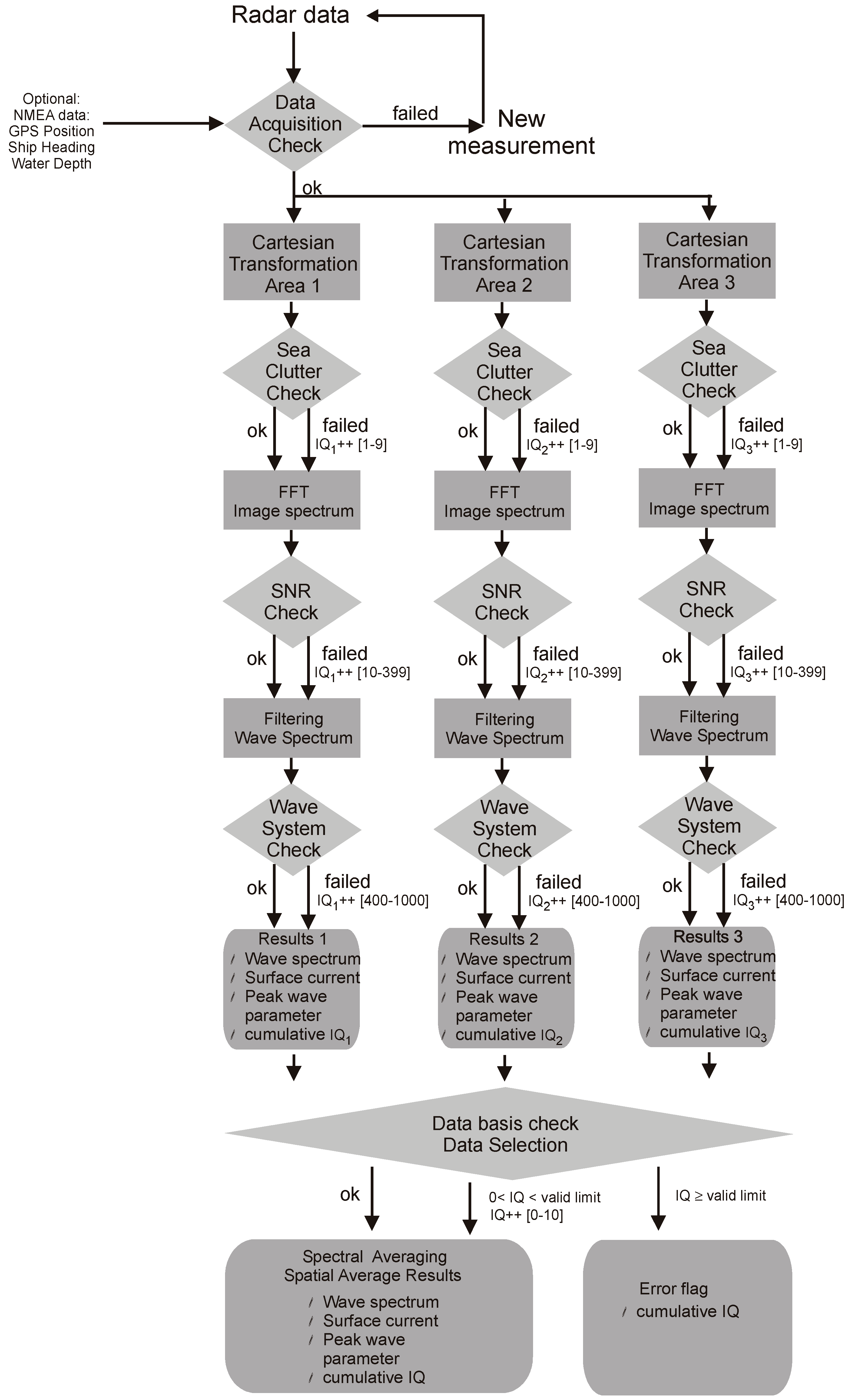
- Data acquisition check: This check verifies if all mandatory information is available.
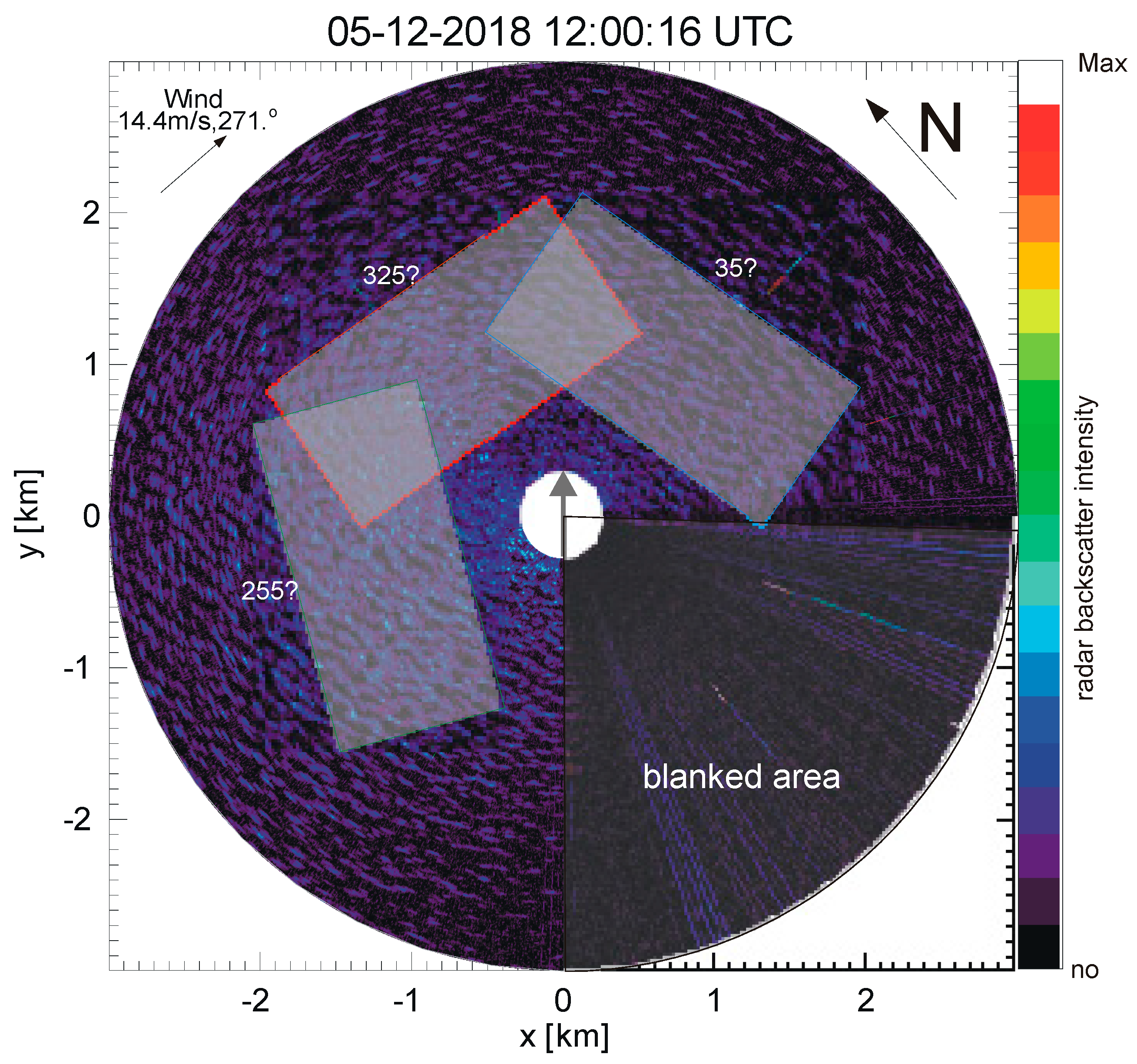
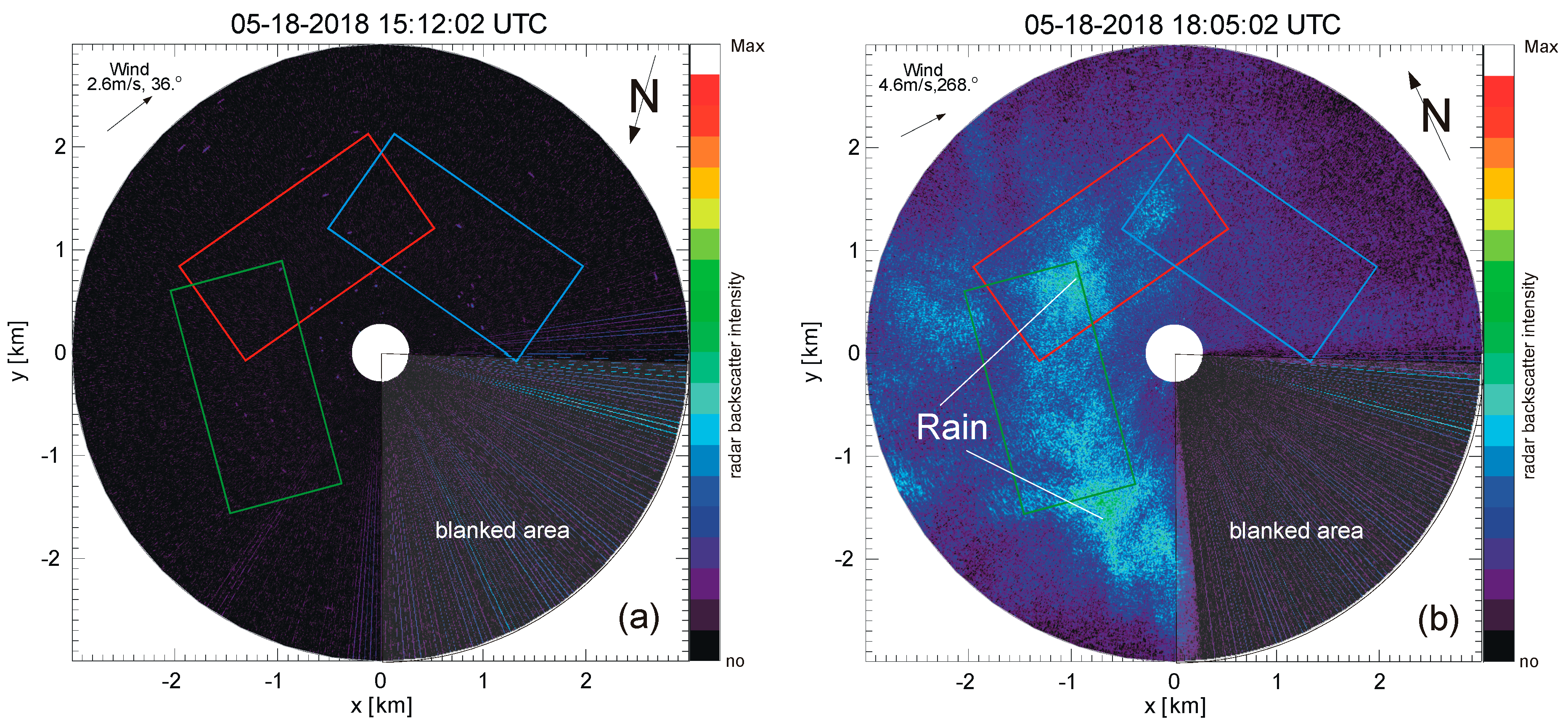
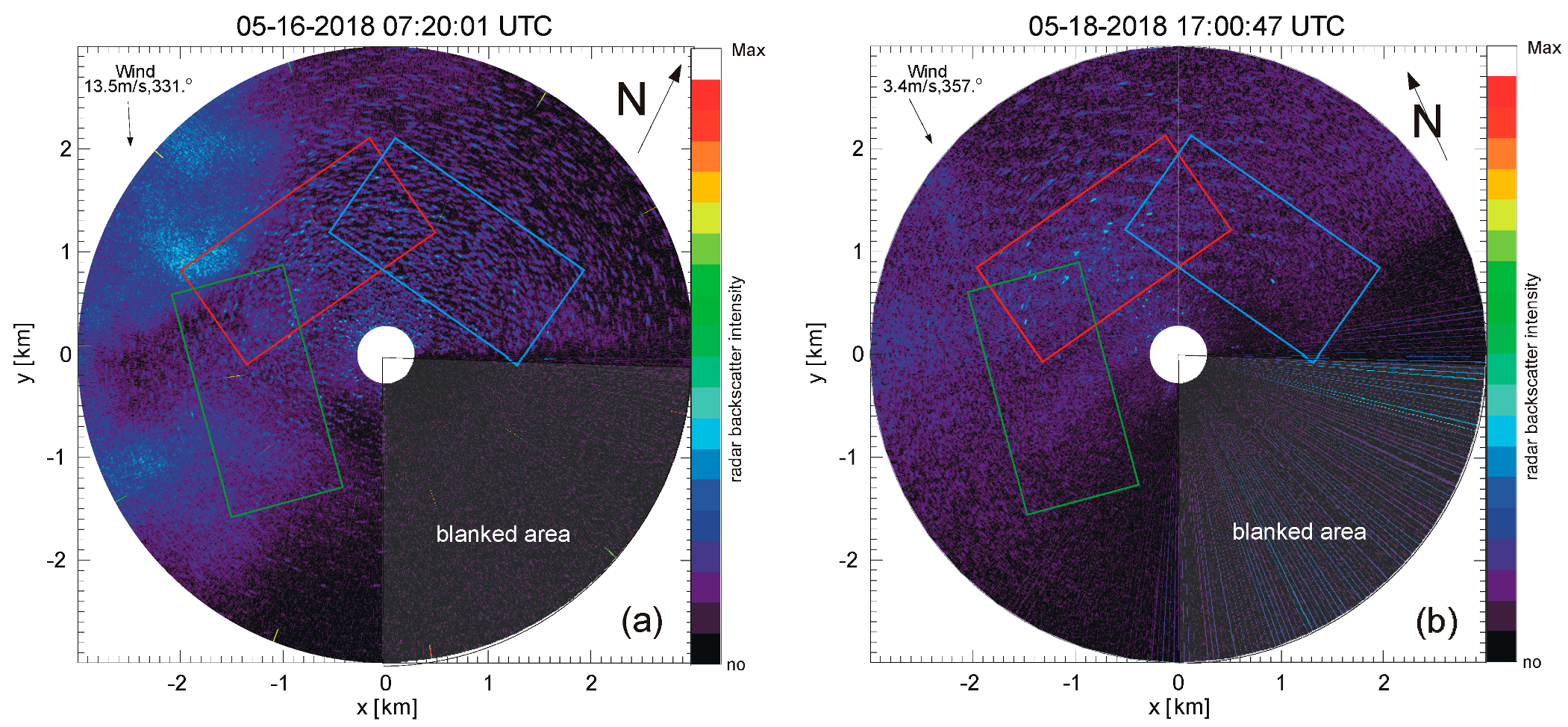
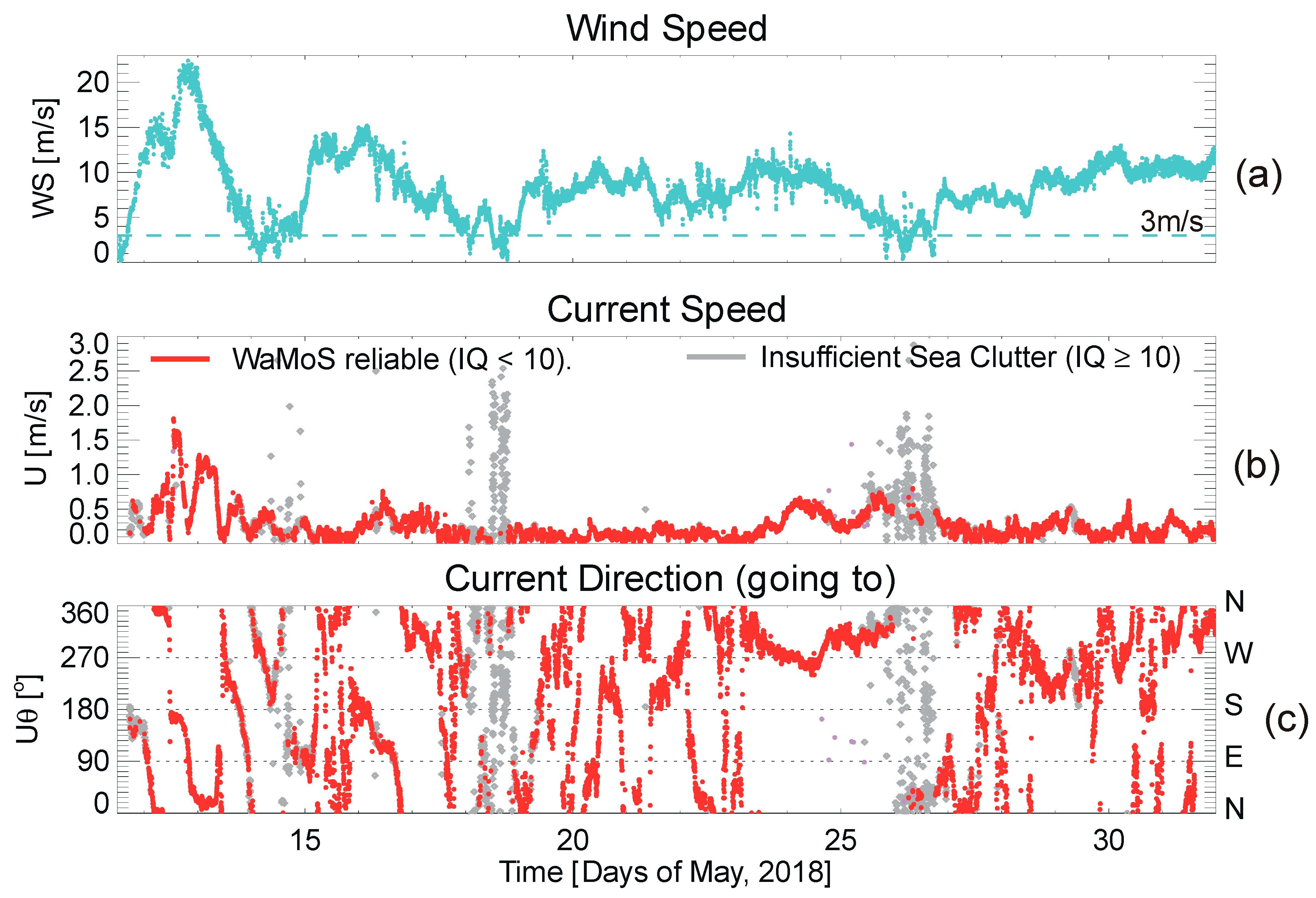
- Sea clutter checks: In this step, the radar raw input is controlled. In cases of insufficient sea clutter information due to no sea state, rain, very low wind conditions (<3 m/s) or missing data sections, the data set is marked with a quality identifier IQ of 0 < IQ < 9.
- SNR-checks: Here, the quality of the separation of signal and noise within the image spectrum is used to evaluate the quality of the current estimate and wave filtering. Data sets which do not pass these checks have potentially unreliable current estimates and are marked with 10 < IQ < 400.
- Wave system checks: When deriving the standard sea state parameters from the frequency direction spectrum , the number of individual wave systems is determined. In cases of more than 5 wave systems, can be regarded as too noisy to give reliable results. In these cases, the resulting data sets are marked with 400 < IQ < 1000.
- Data basis check: For spatial and temporal averages, a minimum of individual measurements is required to obtain a statistically stable result and hence trustful data. All mean data sets with less measurements are marked with 0 < IQ < 10.
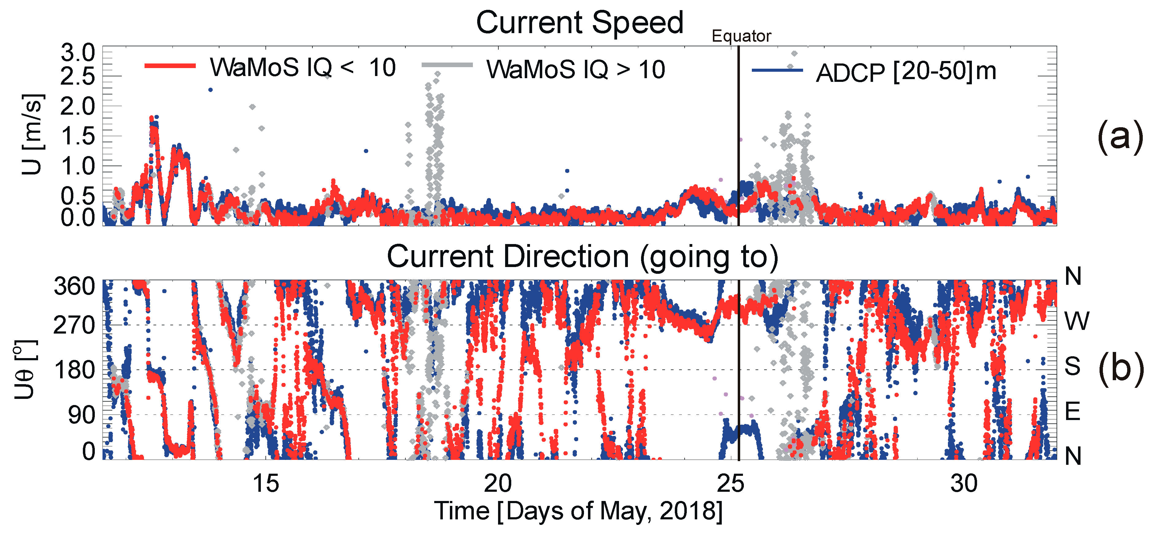
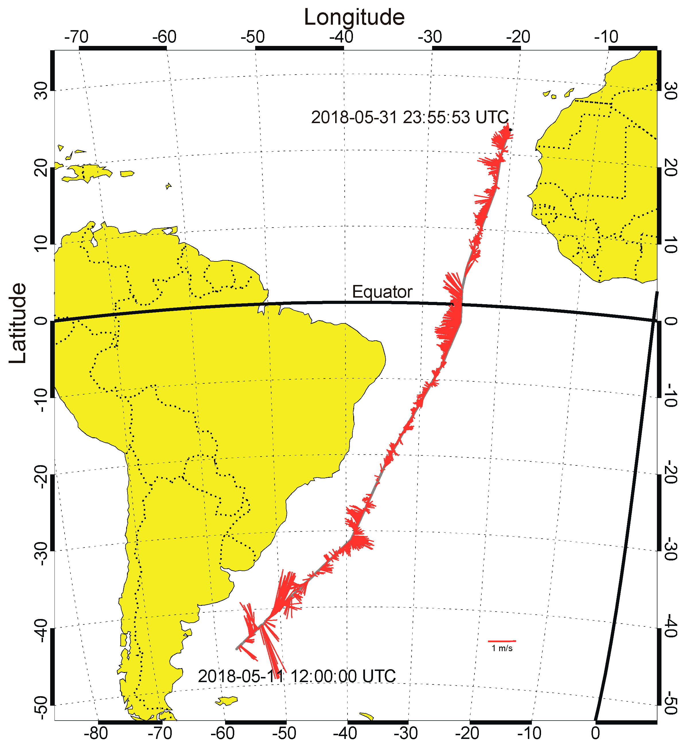
5. Observations During the Cruise
6. Results
7. Summary and Conclusions
Author Contributions
Funding
Acknowledgments
Conflicts of Interest
References
- Oudshoorn, H.M. The use of radar in hydrodynamic surveying. Coast. Eng. Proc. 1960, 59–76. [Google Scholar] [CrossRef]
- Young, I.; Rosenthal, W.; Ziemer, F. A Three-Dimensional Analysis of Marine Radar Images for the Determination of Ocean Wave Directionality and Surface Currents. J. Geophys. Res. 1985, 90, 1049–1059. [Google Scholar] [CrossRef]
- Senet, C.; Seeman, J.; Ziemer, F. The near-surface current velocity determined from image sequences of the sea surface. IEEE Trans. Geosci. Remote Sens. 2001, 39, 492–505. [Google Scholar] [CrossRef]
- Ziemer, F.; Dittmer, J. A system to monitor ocean wave fields. In Proceedings of the Oceans ’94, Brest, France, 13–16 September 1994. [Google Scholar]
- Borge, J.C.N.; Reichert, K.; Dittmer, J. Use of nautical radar as a wave monitoring instrument. Coast. Eng. 1999, 37, 331–342. [Google Scholar] [CrossRef]
- Borge, J.C.N.; Rodrígzues, G.R.; Hessner, K.G.; González, P.I. Inverstion of marine radar images for surface wave analysis. J. Atmos. Ocean. Technol. 2004, 21, 1291–1300. [Google Scholar] [CrossRef]
- Bell, P.S.; Lawrence, J.; Norris, J.V. Determining currents from marine radar data in an extreme current environment at a tidal energy test site. In Proceedings of the IEEE International Geoscience and Remote Sensing Symposium (IGARSS 2012), Munich, Germany, 22–27 July 2012. [Google Scholar]
- Hessner, K.G.; Reichert, K.; Borge, J.C.N.; Stevens, C.; Smith, M. High-resolution X-Band radar measurements of currents, bathymetry and sea state in highly inhomogeneous coastal areas. Ocean. Dyn. 2014, 64, 989–998. [Google Scholar] [CrossRef]
- Hessner, K.G.; Wallbridge, S.; Dolphin, T. Validation of Areal Wave and Current Measurements Based on X-Band Radar. In Proceedings of the 2015 IEEE/OES Eleveth Current, Waves and Turbulence Measurement (CWTM 2015), St. Petersburg, FL, USA, 2–6 March 2015. [Google Scholar]
- Lund, B.; Graber, H.C.; Hessner, K.G.; Williams, N.J. On Shipbord Marin X-Band Radar Near-Surface Current “Calibration”. J. Athmos. Ocean. Technol. 2015, 32, 1928–1944. [Google Scholar] [CrossRef]
- Lund, B.; Collins, C.O., III; Tamura, T.; Graber, H.C. Multi-directional wave spectra from marine X-Band radar. Ocean. Dyn. 2016, 66, 973–988. [Google Scholar] [CrossRef]
- Lund, B.; Zappa, C.J.; Graber, H.C.; Cifuentes-Lorenzen, A. Shipboard Wave Measurments in the Southern Ocean. J. Athmos. Ocean. Technol. 2017, 34, 2113–2126. [Google Scholar] [CrossRef]
- Skolnik, M.I. Introduction to Radar Systems; McGraw-Hill: New York, NY, USA, 1981. [Google Scholar]
- Strass, V. The Expedition PS113 of the Research Vessel POLARSTERN to the Atlantic Ocean in 2018. Berichte zur Polar- und Meeresforschung 2018, 724, 72. [Google Scholar]
- Lund, B.; Graber, H.C.; Tamura, H.C.; Varlamow, S.M.; Collins, C.O., III. A new technique for the retrieval of near-surface vertical current shear from marine X-band radar images. J. Geophys. Res. 2015, 120, 8466–8486. [Google Scholar] [CrossRef]
- Chapman, R.D.; Shay, L.K.; Graber, H.C.; Edson, J.B.; Karachintsev, A.; Trump, C.L.; Ross, D.B. On the accuracy of HR radar surface current measurments: Intercaomparison with ship-based sensors. J. Geophys. Res. 1997, 102, 18.737–18.748. [Google Scholar] [CrossRef]
- Liu, Y.; Weisberg, R.H.; Merz, C.R. Assessment of codar seasonde and wera hf radars in mapping surface currents on the West Floria shelf. J. Atmos. Ocean. Techol. 2014, 31, 1363–1382. [Google Scholar] [CrossRef]
- Williams, A.J. Standards for in Situ current measurement. In Proceedings of the 2015 IEEE/OES Eleveth Current, Waves and Turbulence Measurement (CWTM 2015), St. Petersburg, FL, USA, 2–6 March 2015. [Google Scholar]
- Noris, A.; Wall, A.D.; Bole, A.G.; Dineley, W.O. Radar and ARPA Manual: Radar and Target Tracking for Professional Mariners, Yachtsmen and Users of Marine Radar, 2nd ed.; Elsevier Science: Amsterdam, The Netherlands, 2005; p. 544. [Google Scholar]
- Bell, P.S.; Osler, J.C. Mapping bathymetry using X-band marine radar data recorded from a moving vessel. Ocean. Dyn. 2011, 61, 2141–2156. [Google Scholar] [CrossRef]
- Dean, R.G.; Dalrymple, R.A. Water Wave Meachanics for Engineers and Scientists; World Scientific: Singapore, 1991. [Google Scholar]
- Fischer, J.; Brandt, P.; Dengler, M.; Müller, M.; Symonds, D. Surveying the upper ocean with the ocean surveyor: A new phased array doppler current profiler. J. Atmos. Ocean. Technol. 2003, 20, 742–751. [Google Scholar] [CrossRef]
- Gordon, A.L. Brazil—Malvinas Confluence. Deep Sea Res. 1989, 36, 359–384. [Google Scholar] [CrossRef]
- Ardhuin, F.; Marié, L.; Rascle, N.; Forget, P.; Roland, A. Observation and estimation of Lagrangian, Stokes, and Eulerian currents induced by wind and waves at the sea surface. J. Phys. Oceanogr. 2009, 19, 2820–2838. [Google Scholar] [CrossRef]
- Hessner, K.G.; El-Naggar, S.; Strass, V.; Krägefsky, S.; Witte, H. Evaluation of X-Band MR surfac and ADCP subsurface currents obtaine onboard the German Research Vessel Polarstern during ANT-XXXI expedition 2015/16. In Proceedings of the OCEANS 2017, Anchorage, AK, USA, 18–21 September 2017. [Google Scholar]


| Parameter | Symbol | UE | UN | US | Uθ |
|---|---|---|---|---|---|
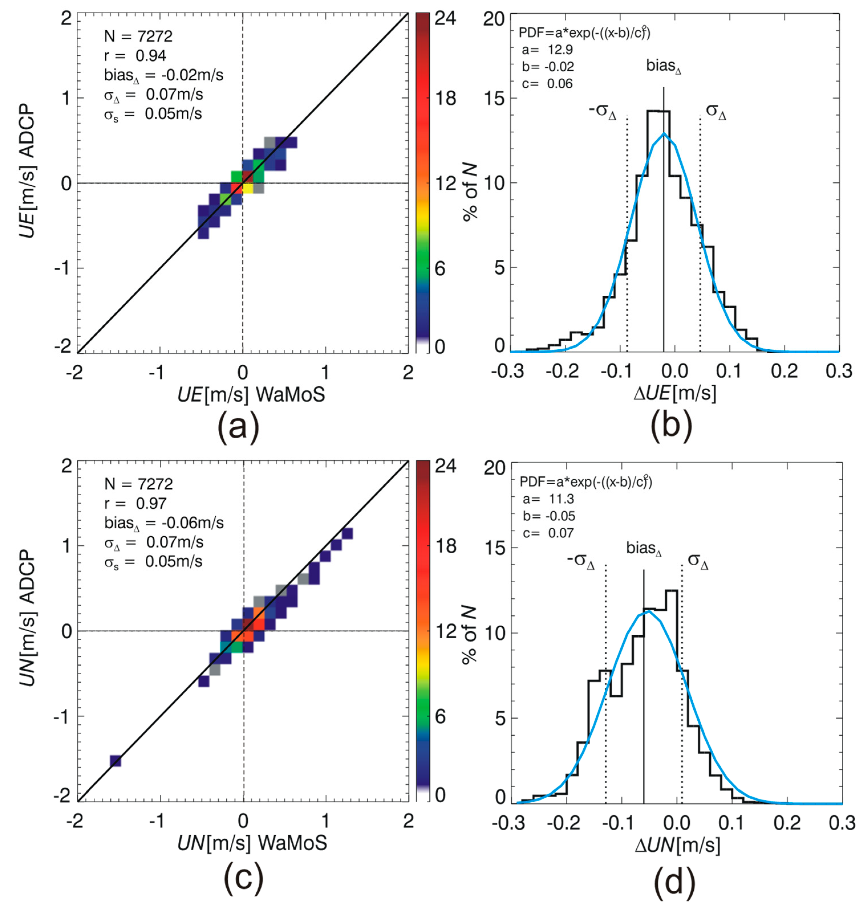
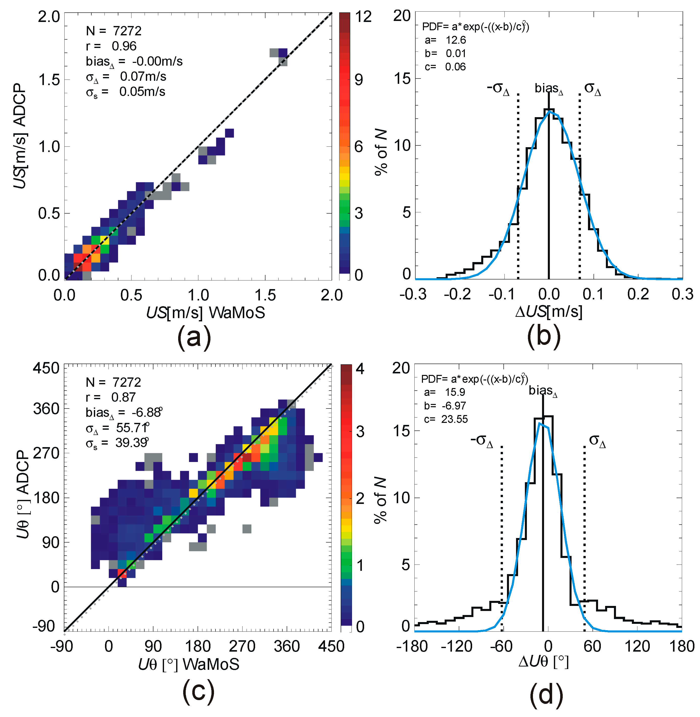
| Number of data sets | N | 7272 | |||
| Correlation coefficient (Equation (1)) | r | 0.94 | 0.97 | 0.96 | 0.87 |
| Bias (Equation (2)) | −0.02 m/s | −0.06 m/s | −0.0004 m/s | −6.88° | |
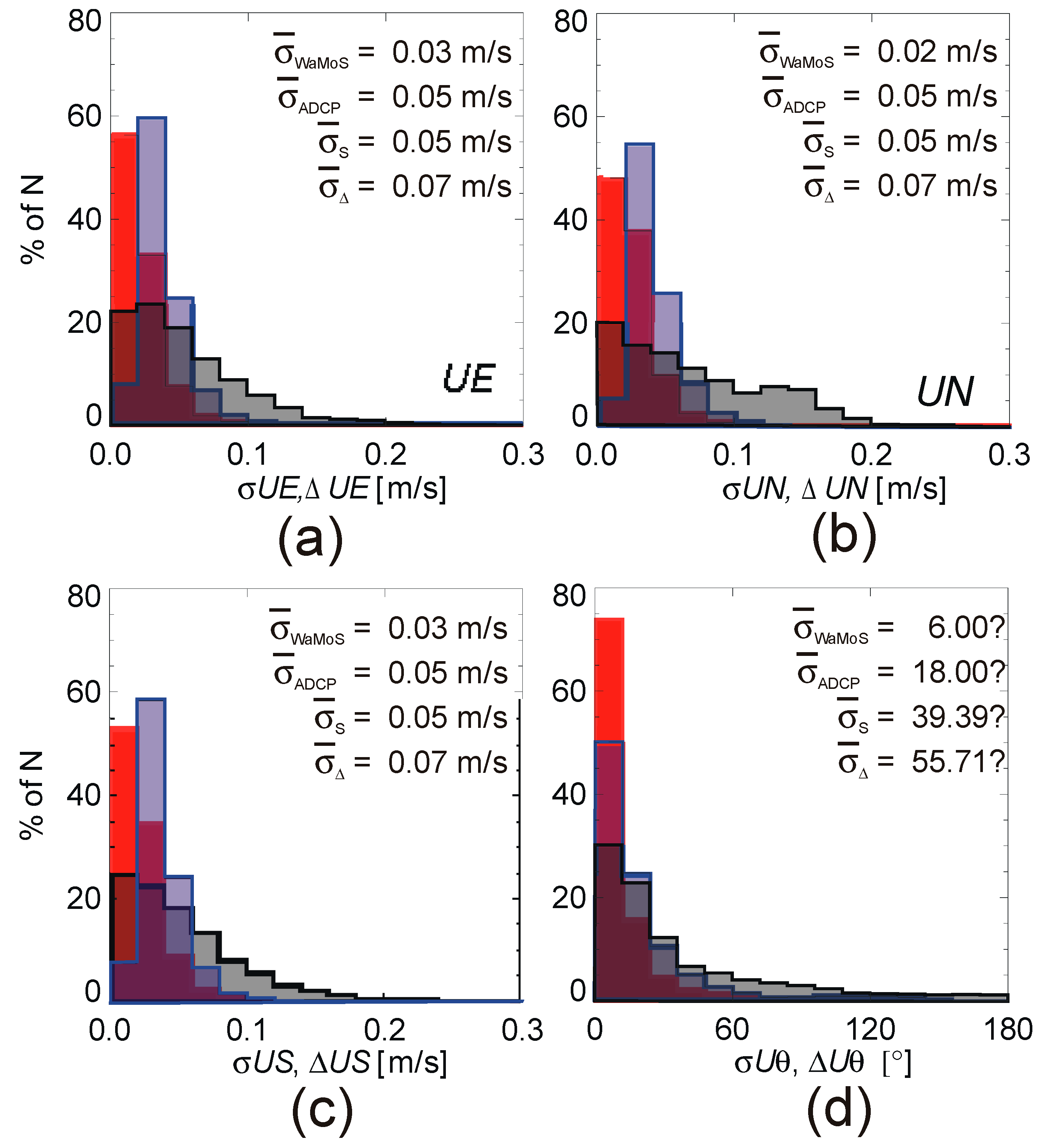
| Total standard deviation of the difference (Equation (3)) | 0.07 m/s | 0.07 m/s | 0.07 m/s | 55.71° | |
| Individual standard deviation (Equation (4)) | 0.05 m/s | 0.05 m/s | 0.05 m/s | 39.39° | |
| Standard deviation of the temporal mean ADCP measurements (Equation (5)) | 0.05 m/s | 0.05 m/s | 0.05 m/s | 18.00° | |
| Standard deviation of the temporal WaMoS®II measurements (Equation (5)) | 0.03 m/s | 0.02 m/s | 0.03 m/s | 6.00° | |
© 2019 by the authors. Licensee MDPI, Basel, Switzerland. This article is an open access article distributed under the terms and conditions of the Creative Commons Attribution (CC BY) license (http://creativecommons.org/licenses/by/4.0/).
Share and Cite
Hessner, K.G.; El Naggar, S.; von Appen, W.-J.; Strass, V.H. On the Reliability of Surface Current Measurements by X-Band Marine Radar. Remote Sens. 2019, 11, 1030. https://doi.org/10.3390/rs11091030
Hessner KG, El Naggar S, von Appen W-J, Strass VH. On the Reliability of Surface Current Measurements by X-Band Marine Radar. Remote Sensing. 2019; 11(9):1030. https://doi.org/10.3390/rs11091030
Chicago/Turabian StyleHessner, Katrin G., Saad El Naggar, Wilken-Jon von Appen, and Volker H. Strass. 2019. "On the Reliability of Surface Current Measurements by X-Band Marine Radar" Remote Sensing 11, no. 9: 1030. https://doi.org/10.3390/rs11091030
APA StyleHessner, K. G., El Naggar, S., von Appen, W.-J., & Strass, V. H. (2019). On the Reliability of Surface Current Measurements by X-Band Marine Radar. Remote Sensing, 11(9), 1030. https://doi.org/10.3390/rs11091030