Estimating Wave Direction Using Terrestrial GNSS Reflectometry

Abstract

The signal-to-noise ratio (SNR) data are part of the global navigation satellite systems (GNSS) observables. In a marine environment, the oscillation of the SNR data can be used to derive reflector heights. Since the attenuation of the SNR oscillation is related to the roughness of the sea surface, the significant wave height (SWH) of the water surface can be calculated from the analysis of the attenuation. The attenuation depends additionally on the relation between the coherent and the incoherent part of the scattered power. The latter is a function of the correlation length of the surface waves. Since the correlation length changes with respect to the direction of the line of sight relative to the wave direction, the attenuation must show an anisotropic characteristic. In this work, we present a method to derive the wave direction from the anisotropy of the attenuation of the SNR data. The method is investigated based on simulated data, as well by the analysis of experimental data from a GNSS station in the North Sea.

1. Introduction

For more than 20 years, reflected global navigation satellite system (GNSS) signals have been used as a tool to observe diverse environmental conditions by estimating the properties of the reflecting surface. In 1993, Martin-Neira [1] first proposed the use of GNSS reflectometry (GNSS-R) in ocean altimetry. Since then, many applications of GNSS-R have been developed, from satellite-based sea surface height (SSH) measurements [2], to land-based observation of soil moisture [3], snow depth [4], and SSH from fixed stations [5] or moving ships [6]. In particular, the interference pattern technique (IPT) has become popular since it uses off-the-shelf equipment, zenith-looking antennas, and standard GNSS observables. Therefore, this technique can be applied to data from many GNSS stations of already existing networks.

Although all GNSS observables are influenced by multipath and can be used for the estimation of the reflector height [7], IPT relates mostly on the analysis of the oscillating structure of the signal-to-noise ratio (SNR) data because it is less influenced by cycle slips or atmospheric refraction as code or carrier phase data. According to [8,9], the frequency of the oscillation is related to the height of the GNSS antenna above a horizontal reflector. The full model [10] also takes into account the attenuation of the SNR signal that depends on the roughness of the reflecting surface. If the reflector is a water surface, the roughness is a measure of the significant wave height (SWH). The authors of [11] have reported that the SWH can be derived from the elevation angle, at which the coherent part of the reflected signal becomes smaller than the incoherent part. It was shown by [12] that the attenuation factor of the oscillating SNR data can be used together with its amplitude and standard deviation to find the elevation angle ε_coh at which the coherence is lost, while [13] have shown that the damping factor of the oscillating SNR data can be used to find the significant wave height.

The authors of [11] compared their experimental results with data derived from the well-established Beckmann–Spizzichino model [14] for scattered reflection from a rough surface. This model describes the mean scattered field as a combination of a coherent and an incoherent part. While both parts depend on the roughness of the water surface, the incoherent part depends additionally on the correlation length of the surface. If the correlation length increases, the incoherent part increases too. This can lead to a domination of the incoherent part and yield a loss of coherence, as well as an increased roughness.

Until now, in the SNR data analysis it was assumed that the correlation length of a sea surface was isotropic. However, a simple gedankenexperiment shows that the correlation length must depend on the wave direction and the direction from which the reflection comes: Consider a simple plane infinite wind-driven wave and define the direction from where the wave comes as the upwind direction and its opposite as the downwind direction. The direction perpendicular to the wave front is than referred to as the cross-wind direction. If we intersect the surface in the upwind or downwind direction and calculate the autocorrelation of the wave heights along the intersection, we will find a correlation length that is related to the wavelength. If we intersect the surface in any off-upwind or off-downwind direction, the wavelength along the intersection will become longer due to the geometrical stretching of the wave height distribution. If the direction of the intersection tends to the cross-wind direction, the correlation length tends to become infinitely long. Although this model is far too simple, it shows that it should be possible to derive the direction of waves from the anisotropy of ε_coh.

The aim of this work is to demonstrate the possibility to derive the direction of waves from the analysis of GNSS SNR data. In Section 2, the basic theory of SNR data analysis and the scattered reflection model from Beckmann and Spizzichino is explained and discussed. Section 3 presents an investigation of the suggested method based on simulations of wave fields. In Section 4, real data from a GNSS-equipped tide gauge in the North Sea are analyzed and compared to data from a wave buoy and observations of wind directions. Section 5 concludes our findings.

2. Theoretical Background

2.1. Analysis of SNR Data

The analysis in this work is based on the interference of a direct and a reflected signal that creates a characteristic oscillation in the signal-to-noise ratio (SNR). According to the full model from [10], the SNR is a combination of the direct and the reflected power related to the noise power. Under the assumption of a plane reflecting surface, the SNR can be decomposed into a trend and interference fringes that are attenuated with respect to the elevation angle:

$$\begin{array}{cc}\hfill \mathrm{S}\mathrm{N}\mathrm{R}=& \mathrm{t}\mathrm{r}\mathrm{e}\mathrm{n}\mathrm{d}+\mathrm{a}\mathrm{t}\mathrm{t}\mathrm{e}\mathrm{n}\mathrm{u}\mathrm{a}\mathrm{t}\mathrm{i}\mathrm{o}\mathrm{n}\cdot \mathrm{o}\mathrm{s}\mathrm{c}\mathrm{i}\mathrm{l}\mathrm{l}\mathrm{a}\mathrm{t}\mathrm{i}\mathrm{o}\mathrm{n}\hfill \\ \hfill \mathrm{t}\mathrm{r}\mathrm{e}\mathrm{n}\mathrm{d}=& {\mathrm{c}}_0+{\mathrm{c}}_1\mathrm{t}+{\mathrm{c}}_2{\mathrm{t}}^2+\dots \hfill \\ \hfill \mathrm{a}\mathrm{t}\mathrm{t}\mathrm{e}\mathrm{n}\mathrm{u}\mathrm{a}\mathrm{t}\mathrm{i}\mathrm{o}\mathrm{n}=& {\mathrm{e}}^{-{\mathrm{k}}^2{\mathrm{d}}^2{\sin }^2\mathsf{\epsilon }},\mathrm{k}=2\mathsf{\pi }/\mathsf{\lambda }\hfill \\ \hfill \mathrm{o}\mathrm{s}\mathrm{c}\mathrm{i}\mathrm{l}\mathrm{l}\mathrm{a}\mathrm{t}\mathrm{i}\mathrm{o}\mathrm{n}=& \mathrm{A}\mathrm{m}\mathrm{p}\cdot \cos (4\mathsf{\pi }/\mathsf{\lambda }{\mathrm{h}}_{\mathrm{r}\mathrm{e}\mathrm{f},\mathrm{t}}\sin \mathsf{\epsilon }+{\mathsf{\varphi }}_0)\hfill \end{array}$$

(1)

Here, c₀, c₁ and c₂ are the unknown parameters of a polynomial trend function of the time t, k is the wave number, λ is the wave length of the GNSS signal, d is the unknown damping coefficient, ε is the complementary angle of the incidence angle, Amp is the unknown amplitude of the SNR, and ${\mathsf{\varphi }}_0$ is the unknown phase offset of the oscillation. The oscillation is governed by the reflector height h_ref,t, which is the height of the antenna above the reflecting surface at the position of the specular point, which might be variable in time. With h_APC as the height of the antenna phase centre (APC) in a certain height datum and h_tide,t as time-variable water surface height in the same height datum, h_ref,t can be described as

$${\mathrm{h}}_{\mathrm{r}\mathrm{e}\mathrm{f},\mathrm{t}}={\mathrm{h}}_{\mathrm{A}\mathrm{P}\mathrm{C}}-{\mathrm{h}}_{\mathrm{t}\mathrm{i}\mathrm{d}\mathrm{e},\mathrm{t}}+\mathrm{d}{\mathrm{h}}_{\mathrm{s}\mathrm{p}\mathrm{h}\mathrm{e}\mathrm{r}\mathrm{e},\mathrm{t}}$$

(2)

Since specular points can lie in a distance of several hundreds of meters away from the position of the antenna, the term dh_sphere,t corrects for the surface curvature in a spherical approximation. The complementary angle of the incidence angle ε defers from the elevation angle of the satellite due to the curvature of the reflecting surface and can be calculated according to [6,15]. The tropospheric refraction can be considered by a correction of ε derived from an astronomic refraction model [16,17,18,19].

The unknowns in Equation (1) can be derived from different methods. If h_APC and h_tide in Equation (2) are known, a non-linear least-squares adjustment for every satellite can be applied to estimate the individual unknown parameters. If h_ref is likewise unknown, it can be assumed that it is constant for all satellites observed at the same time. Due to the multimodality of h_ref, this parameter can be included in the non-linear adjustment only if good initial values are available. Otherwise, optimization techniques might be applied [20].

The amplitude at a specific angle ε can be calculated from the attenuation and the amplitude Amp in Equation (1) as

$$\mathrm{A}\mathrm{m}{\mathrm{p}}_{\mathsf{\epsilon }}=\mathrm{A}\mathrm{m}\mathrm{p}\cdot {\mathrm{e}}^{-4{\mathrm{k}}^2{\mathrm{d}}^2{\sin }^2\mathsf{\epsilon }}$$

(3)

While the angle ε increases, Amp_ε becomes small in comparison to the noise of the SNR data and above a certain angle, it disappears in the noise. It is assumed that this is the cutoff angle ε_coh, at which the coherence is lost. The threshold at which the loss of coherence is assumed is a matter of definition. We suppose to use a threshold that is related to the standard deviation of the SNR data σ_SNR derived from the non-linear least-squares adjustment multiplied by a factor f. Under these assumptions the coherence is lost if

$$\mathrm{A}\mathrm{m}{\mathrm{p}}_{\mathsf{\epsilon }}\le \mathrm{f}\cdot {\mathsf{\sigma }}_{\mathrm{S}\mathrm{N}\mathrm{R}}$$

(4)

The cutoff angle ε_coh is therefore deduced from Equations (3) and (4) as

$${\mathsf{\epsilon }}_{\mathrm{c}\mathrm{o}\mathrm{h}}=\arcsin \sqrt{\ln (\mathrm{f}\cdot {\mathsf{\sigma }}_{\mathrm{S}\mathrm{N}\mathrm{R}}/\mathrm{A}\mathrm{m}\mathrm{p})/(-4{\mathrm{k}}^2{\mathrm{d}}^2)},\mathrm{f}\mathrm{o}\mathrm{r}\mathrm{f}\cdot {\mathsf{\sigma }}_{\mathrm{S}\mathrm{N}\mathrm{R}}<\mathrm{A}\mathrm{m}\mathrm{p}$$

(5)

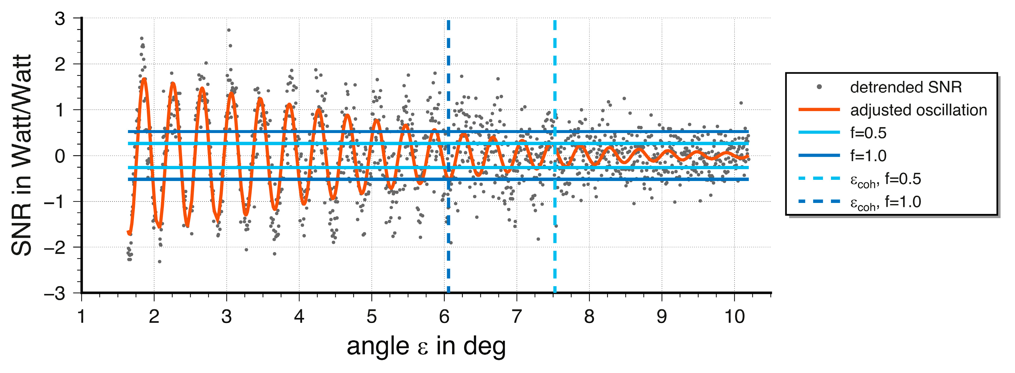
Figure 1 depicts typical trend-reduced SNR data, based on the data used in Section 4. We plotted the threshold for a factor of 0.5 and 1.0 together with the resulting cutoff angle ε_coh. The actual value of the factor f is of minor importance for the investigation of the anisotropic behavior of the cutoff angle ε_coh as long as it is constant for all satellites involved in the investigation of a particular sea state.

2.2. Scattered Reflection

According to [11], the scattered reflection from a rough surface can be described by the Beckmann–Spizzichino model. It should be mentioned here that the description used in this work neglects shadowing or multiple scattering, and can therefore only yield approximate results. Nevertheless, the model can be used to investigate the fundamental relations between surface roughness, correlation length, and loss of coherence.

We use here the notation from [21]. There, the mean scattered power $<{\mathrm{E}}_2{\mathrm{E}}_2^{*}>$ of the reflection from a rough surface is described based on the scattered power $<{\left|{\mathrm{E}}_{2\mathrm{s}\mathrm{s}}\right|}^2>$ of the reflection from a smooth perfectly conducting surface as

$$<{\mathrm{E}}_2{\mathrm{E}}_2^{*}>=<{\left|{\mathrm{E}}_{2\mathrm{s}\mathrm{s}}\right|}^2>\cdot {\mathrm{e}}^{-\mathrm{g}}({\mathsf{\rho }}_0^2+\frac{\mathsf{\pi }{\mathrm{T}}^2{\mathrm{D}}^2}{\mathrm{A}}{\displaystyle \sum _{\mathrm{m}=1}^{\infty }\frac{{\mathrm{g}}^{\mathrm{m}}}{\mathrm{m}!\mathrm{m}}}{\mathrm{e}}^{-{\mathrm{v}}_{\mathrm{x}\mathrm{y}}^2\frac{{\mathrm{T}}^2}{4\mathrm{m}}})$$

(6)

where

$$\begin{array}{l}\mathrm{g}={\left(2\mathsf{\pi }\frac{{\mathsf{\sigma }}_{\mathrm{h}}}{\mathsf{\lambda }}(\cos {\mathsf{\theta }}_{\mathrm{i}}+\cos {\mathsf{\theta }}_{\mathrm{r}})\right)}^2\\ {\mathsf{\rho }}_0=\sin \mathrm{c}({\mathrm{v}}_{\mathrm{x}}\mathrm{X})\sin \mathrm{c}({\mathrm{v}}_{\mathrm{y}}\mathrm{Y})\\ \mathrm{D}=\left(\frac{1+\cos {\mathsf{\theta }}_{\mathrm{i}}\cos {\mathsf{\theta }}_{\mathrm{r}}-\sin {\mathsf{\theta }}_{\mathrm{i}}\sin {\mathsf{\theta }}_{\mathrm{r}}\cos {\mathsf{\varphi }}_{\mathrm{r}}}{\cos {\mathsf{\theta }}_{\mathrm{i}}(\cos {\mathsf{\theta }}_{\mathrm{i}}+\cos {\mathsf{\theta }}_{\mathrm{r}})}\right)\\ {\mathrm{v}}_{\mathrm{x}}=\mathrm{k}(\sin {\mathsf{\theta }}_{\mathrm{i}}-\sin {\mathsf{\theta }}_{\mathrm{r}}\cos {\mathsf{\varphi }}_{\mathrm{r}})\mathrm{x}\\ {\mathrm{v}}_{\mathrm{y}}=\mathrm{k}(\sin {\mathsf{\theta }}_{\mathrm{r}}\sin {\mathsf{\varphi }}_{\mathrm{r}})\mathrm{y}\\ {\mathrm{v}}_{\mathrm{x}\mathrm{y}}=\sqrt{{\mathrm{v}}_{\mathrm{x}}^2+{\mathrm{v}}_{\mathrm{y}}^2}\end{array}$$

Here, σ_h is the standard deviation of the surface heights. For water surfaces, it is assumed to be approximately a quarter of the SWH [22]. Furthermore, λ is the wavelength of the GNSS signal, T is the correlation length of the reflecting surface, θ_i is the incidence angle with θ_i = 90°-ε, θ_r is the reflecting angle, ϕ_r is the azimuth of the reflection, X and Y are the dimensions of the reflecting area, A in the coordinate direction x and y, and k is again the wave number of the GNSS signal. We are interested in the scattered reflection in the direction of a specular reflection. Therefore, the incidence angle is equal to the reflecting angle and the azimuth of the reflection becomes zero. Since v_x and v_y become zero and D is 1 for this case, Equation (6) simplifies to

$$<{\mathrm{E}}_2{\mathrm{E}}_2^{*}>=<{\left|{\mathrm{E}}_{2\mathrm{s}\mathrm{s}}\right|}^2>{\mathrm{e}}^{-\mathrm{g}}(1+\frac{\mathsf{\pi }{\mathrm{T}}^2}{\mathrm{A}}{\displaystyle \sum _{\mathrm{m}=1}^{\infty }\frac{{\mathrm{g}}^{\mathrm{m}}}{\mathrm{m}!\mathrm{m}}})$$

(7)

Similar to [11], the first term in the bracket in Equation (7) governs the coherent part while the second term governs the incoherent part. Hence, if the term

$$\mathrm{i}\mathrm{n}\mathrm{c}\mathrm{o}\mathrm{h}=\frac{\mathsf{\pi }{\mathrm{T}}^2}{\mathrm{A}}{\displaystyle \sum _{\mathrm{m}=1}^{\infty }\frac{{\mathrm{g}}^{\mathrm{m}}}{\mathrm{m}!\mathrm{m}}}$$

(8)

becomes larger than the term coh = 1, the incoherent part dominates the mean scattered power. If the relation between incoh and coh reaches a particular value, the corresponding angle ε can be stated as the cutoff angle ε_coh. In accordance with [11] we use a value of 1 for the relation in this work.

The term incoh depends partly on the geometry of the scattered reflection since A is set as the area of the Fresnel zone. This depends on the reflector height and the angle ε, which also governs parameter g. Additionally, incoh depends on the sea state because Equation (8) contains the standard deviation of the water surface heights and the correlation length T of the surface. There is no firm definition for a value of the correlation length, but it can be stated as the distance at which the correlation coefficient of the autocorrelation function of the surface height falls below a certain threshold. For real sea surfaces, the surface heights are mainly a result of the wind influence. Hence, the correlation length will be correlated with SWH. It is clear that the correlation length cannot become zero for such surfaces.

Equation (8) cannot be reformulated to express the elevation angle explicitly as a function of T and incoh. Therefore, we applied Newton’s method to find the cutoff elevation angles at which incoh equals 1. The necessary derivate of Equation (8) was derived from numerical differentiation.

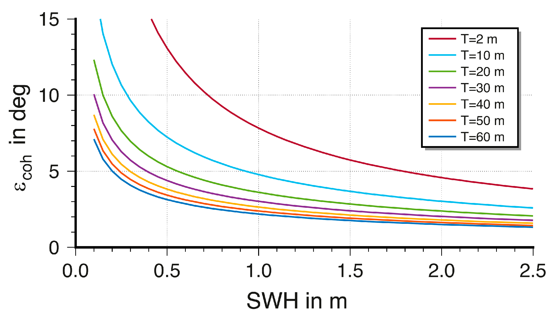
Figure 2 presents the resulting cutoff angle ε_coh for correlation lengths between 2 to 60 m, and for different SWH at a reflector height of 12.3 m. It can be seen that for a particular SWH the cutoff angle ε_coh reaches values of remarkable differences in dependence of the correlation length T. Hence, it should be possible to derive the wave direction if the cutoff angle can be derived from Equation (5) in several azimuthal directions and if the differences in the correlation length are large enough in these azimuthal directions. To clarify the range of the correlation length for sea surfaces, simulated wave fields will be used in Section 3.

3. Simulations

3.1. Waves

Wave fields of the sea surface from the real world are rarely available and do not allow for control of the influencing parameters. Therefore, simulations of a wave field can be used for investigations, but the example of a plane wave field from the introduction is much too simple to allow for the exploration of the range of the correlation length. Hence, more realistic wave fields of the sea surface must be constructed.

Simulations of the three-dimensional height distribution of a sea surface are needed for scientific purposes, such as research on underwater inertial navigation system [23] or computer graphics programming which provide visual effects in print media or films [24]. Here, we used a model that takes into account the stochastic, but directional nature, of the wind-driven waves by representing them as Gaussian stationary and ergodic processes. Consequently, they can be calculated as an infinite sum of simple cosine waves that propagate into azimuthal directions with variable amplitudes, frequencies, and initial phases:

$$\mathrm{H}(\mathrm{x},\mathrm{y})={\displaystyle \sum _{\mathrm{i}=1}^{\infty }{\displaystyle \sum _{\mathrm{j}=1}^{\infty }{\mathrm{A}}_{\mathrm{i},\mathrm{j}}\cos ({\mathrm{k}}_{\mathrm{i}}\mathrm{x}\cos {\mathsf{\theta }}_{\mathrm{j}}}}+{\mathrm{k}}_{\mathrm{i}}\mathrm{y}\sin {\mathsf{\theta }}_{\mathrm{j}}+{\mathsf{\phi }}_{\mathrm{i}\mathrm{j}})$$

(9)

Here, k_i = ω_i²/g is the deep water wave number at angular frequency ω_i, while g is the gravitational acceleration. ${\mathsf{\theta }}_{\mathrm{j}}$ is the direction of the elementary wave and ${\mathsf{\phi }}_{\mathrm{i}\mathrm{j}}$ is a random initial phase. The amplitude ${\mathrm{A}}_{\mathrm{i},\mathrm{j}}$ can be derived approximately from a directional wave spectrum as [25]

$${\mathrm{A}}_{\mathrm{i},\mathrm{j}}\approx \sqrt{2\mathrm{S}({\mathsf{\omega }}_{\mathrm{i}},{\mathsf{\theta }}_{\mathrm{j}})\Delta {\mathsf{\omega }}_{\mathrm{i}}\Delta {\mathsf{\theta }}_{\mathrm{j}}}$$

(10)

where $\Delta {\mathsf{\omega }}_{\mathrm{i}}$ is an increment of ${\mathsf{\omega }}_{\mathrm{i}}$ and $\Delta {\mathsf{\theta }}_{\mathrm{i}}$ is one of ${\mathsf{\theta }}_{\mathrm{i}}$. $\mathrm{S}({\mathsf{\omega }}_{\mathrm{i}},{\mathsf{\theta }}_{\mathrm{j}})$ is the directional power spectrum that is composed by a power spectrum $\mathrm{S}({\mathsf{\omega }}_{\mathrm{i}})$ and a directionality function $\mathrm{D}({\mathsf{\theta }}_{\mathrm{j}})$ as

$$\mathrm{S}({\mathsf{\omega }}_{\mathrm{i}},{\mathsf{\theta }}_{\mathrm{j}})=\mathrm{S}({\mathsf{\omega }}_{\mathrm{i}})\mathrm{D}({\mathsf{\theta }}_{\mathrm{j}})$$

(11)

From the manifold of available power spectra, we used the JONSWAP spectrum [26] that is a modification of the Pierson–Moskowitz spectrum [27] for fetch-limited scenarios. This spectrum is based on observations at the North Sea, the area of the experimental data that will be used in Section 4. Here, we applied the formulation based on SWH and the wave peak period T_p [22].

$$\mathrm{S}(\mathsf{\omega })={\mathrm{A}}_{\mathsf{\gamma }}\frac{5}{16}\mathrm{S}\mathrm{W}{\mathrm{H}}^2{\mathsf{\omega }}_{\mathrm{p}}^4{\mathsf{\omega }}^{-5}\exp \left(-\frac{5}{4}{\left(\frac{\mathsf{\omega }}{{\mathsf{\omega }}_{\mathrm{p}}}\right)}^{-4}\right){\mathsf{\gamma }}^{\exp \left(-0.5{\left(\frac{\mathsf{\omega }-{\mathsf{\omega }}_{\mathrm{p}}}{\mathsf{\sigma }{\mathsf{\omega }}_{\mathrm{p}}}\right)}^2\right)}$$

(12)

where ${\mathsf{\omega }}_{\mathrm{p}}=2\mathsf{\pi }/{\mathrm{T}}_{\mathrm{p}}$, ${\mathrm{A}}_{\mathsf{\gamma }}=1-0.287\ln \mathsf{\gamma }$ and $\mathsf{\gamma }=3.3$. The spectral width parameter $\mathsf{\sigma }$ must be taken as 0.07 if $\mathsf{\omega }\le {\mathsf{\omega }}_{\mathrm{p}}$ or 0.09 if $\mathsf{\omega }>{\mathsf{\omega }}_{\mathrm{p}}$. We used the directional function proposed by ITTC (International Towing Tank Conference) [23]

$$\mathrm{D}({\mathsf{\theta }}_{\mathrm{j}})=\frac{2}{\mathsf{\pi }}{\cos }^2{\mathsf{\theta }}_{\mathrm{j}},\left|{\mathsf{\theta }}_{\mathrm{j}}\right|\le \frac{\mathsf{\pi }}{2}$$

(13)

The simulations were carried out for $0.1\le {\mathsf{\omega }}_{\mathrm{i}}\le 6.1$ Hz with an increment of $\Delta {\mathsf{\omega }}_{\mathrm{i}}=0.2$ Hz, where the main wave direction was set to zero, resulting in a west-to-east downwind direction. Hence, ${\mathsf{\theta }}_{\mathrm{j}}$ in Equations (9) and (13) are the directions of the spread of the wave. The increment $\Delta {\mathsf{\theta }}_{\mathrm{i}}$ was set as one-tenth of the range from a minimum and a maximum wave direction ${\mathsf{\theta }}_{\min }$ and ${\mathsf{\theta }}_{\max }$.

To provide realistic simulations, the parameters for wave peak period T_p, as well as for ${\mathsf{\theta }}_{\min }$ and ${\mathsf{\theta }}_{\max }$, were derived from real data observed over a period of two months at the wave buoy ElbeWR in the North Sea at the Outer Elbe that was deployed by the German Federal Maritime and Hydrographic Agency (Bundesamt für Seeschifffahrt und Hydrographie, BSH). Besides other data, the buoy provides SWH, peak periods, wave principal directions, and the wave directional spreading with a temporal resolution of 30 min. 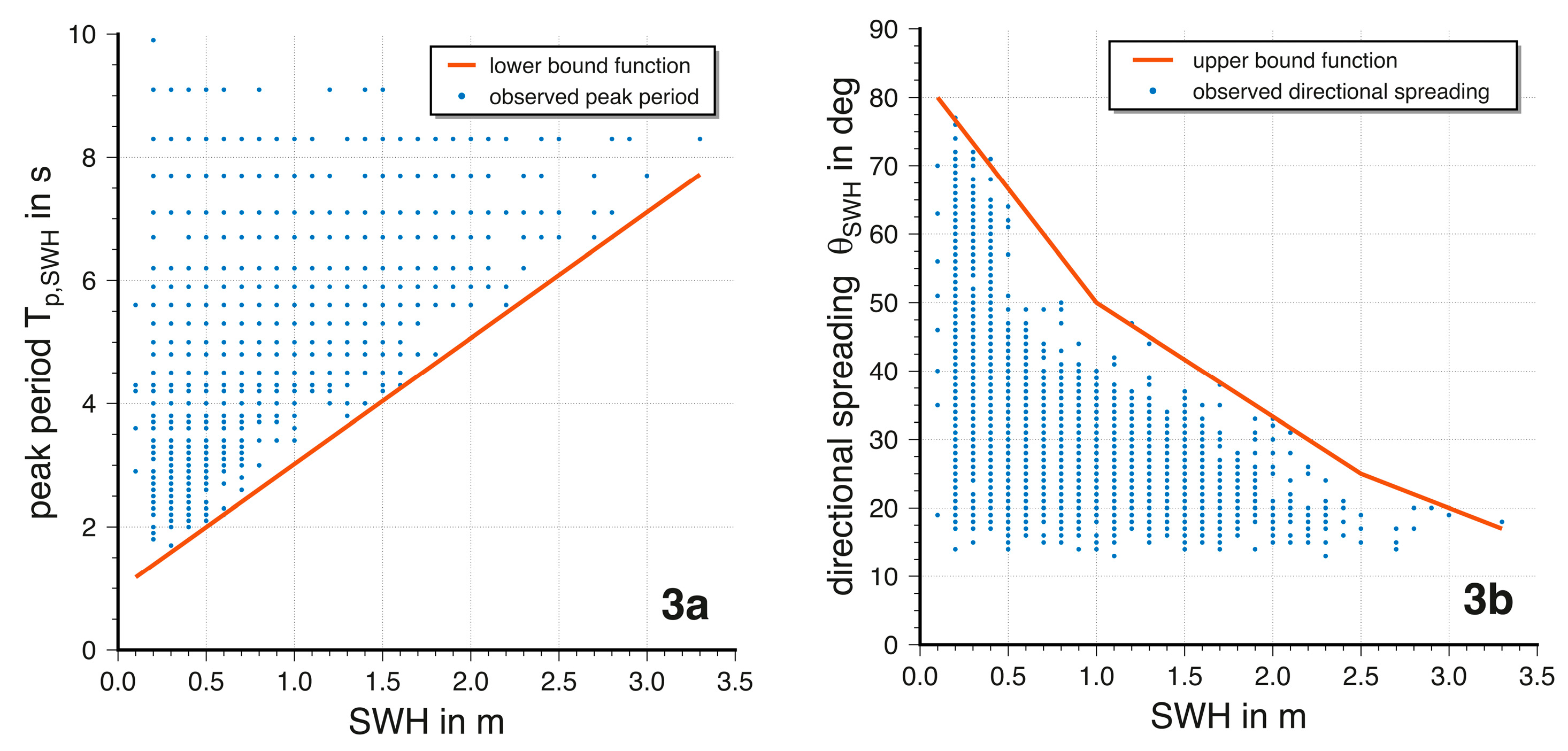Figure 3 depicts observed data for peak periods (a) and directional spreading (b). The peak period does not fall below a certain value for a specific SWH. Hence, a linear function was fitted to derive the wave peak period T_p,SWH as a function of SWH, which will be used for the simulations. Likewise, the directional spreading does rarely exceed the plotted upper bound from which a piecewise linear function is derived. The directional spreading ${\mathsf{\theta }}_{\mathrm{S}\mathrm{W}\mathrm{H}}$ resulting from this function is used to define the minimal and a maximal wave direction as ${\mathsf{\theta }}_{\min }=-{\mathsf{\theta }}_{\mathrm{S}\mathrm{W}\mathrm{H}}/2$ and ${\mathsf{\theta }}_{\max }={\mathsf{\theta }}_{\mathrm{S}\mathrm{W}\mathrm{H}}/2$. It should be stated here, that the derived functions do not represent any physical relation between SWH and the peak period or the directional spreading, respectively. These functions can only be used to derive values for these parameters for the simulation of different wave fields.

The wave field was simulated for a 1 × 1 m grid with an extent of 1000 m for both x and y direction. The range of SWH was set to be between 0.1 m and 2.5 m with an increment of 0.2 m. To avoid too smooth surfaces for small SWH values, we added a normally distributed value with a mean of zero and a standard deviation of s = 5 cm. Due to this, and since the initial phase ${\mathsf{\phi }}_{\mathrm{i}\mathrm{j}}$ from Equation (9) was introduced as an evenly distributed random value within the range of 0 to 2π, the simulated wave field was a random result. For every SWH, we carried out 100 simulations. 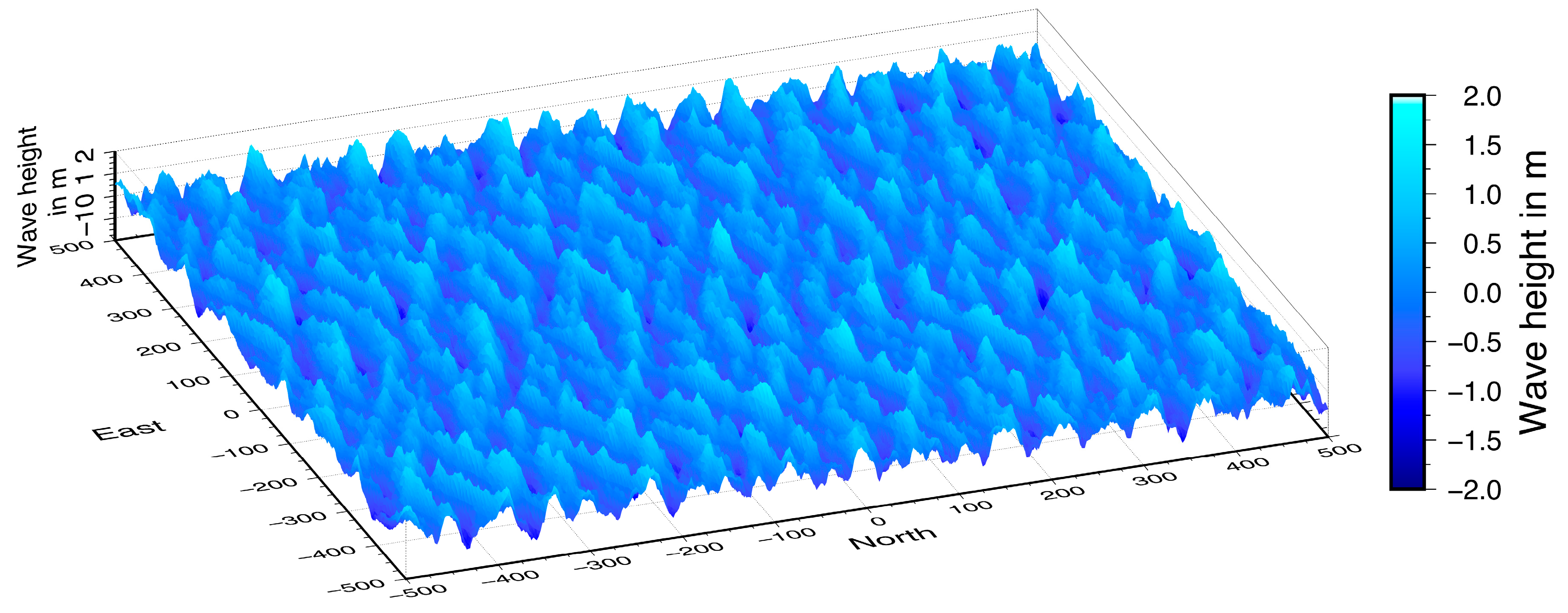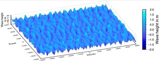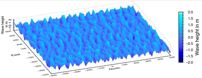Figure 4 presents an arbitrarily selected wave field derived for a SHW of 2.5 m.

3.2. Calculation of Wave Direction

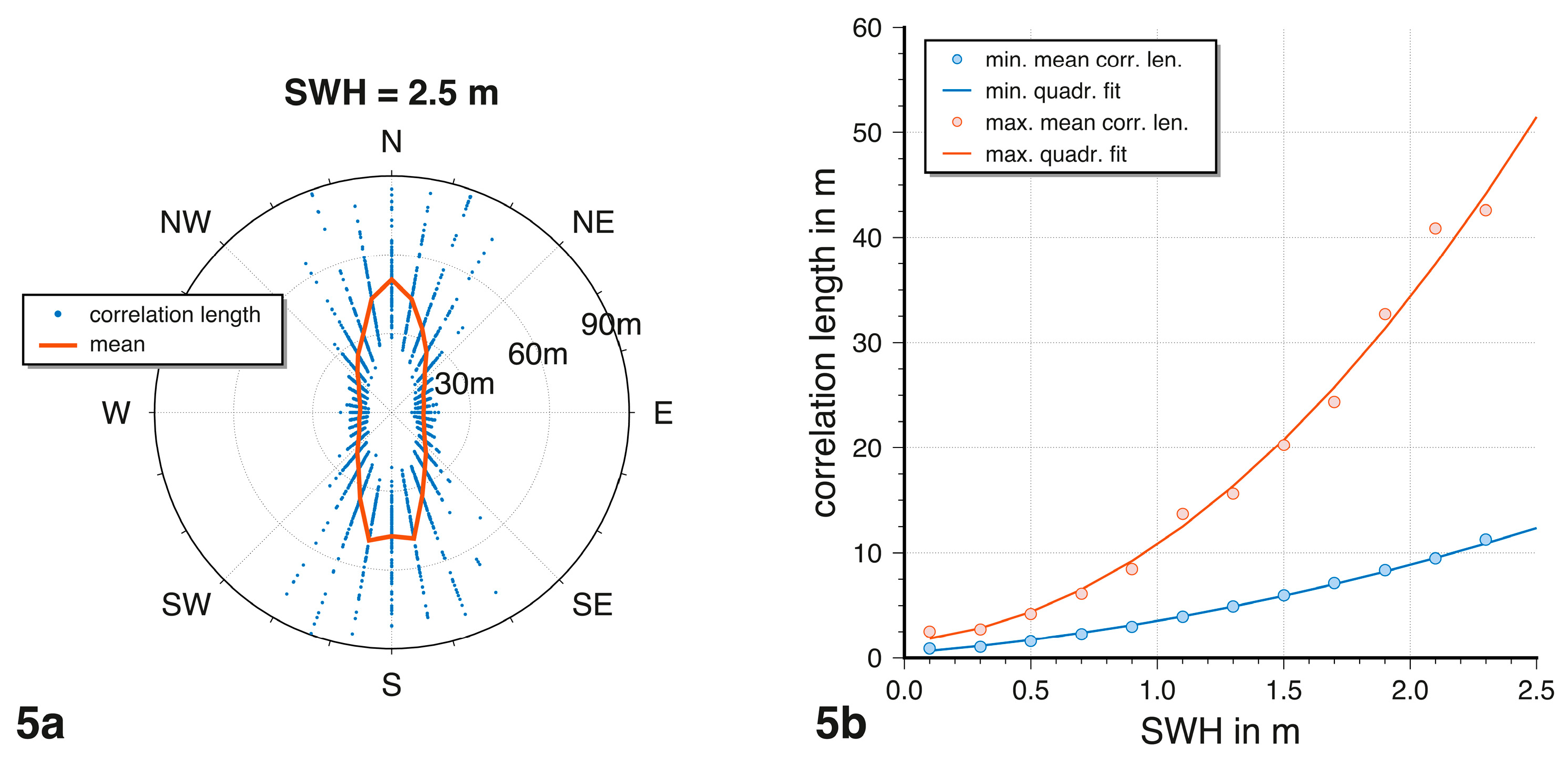
For every simulated wave field, we calculated the autocorrelation function for different azimuthal directions. To do so, we interpolated the wave heights along intersections in azimuth ranging from 0° to 350° with an increment of 10°. Since the autocorrelation function shows the behavior of a damped cosine function [28], we defined the correlation length as the distance at which the autocorrelation becomes zero for the first time. The resulting 100 correlation lengths for a SWH of 2.5 m are plotted in Figure 5a together with the average value for the specific azimuth. The maximum and minimum average correlation length for all SWH are presented in Figure 5b. For both minimum and maximum values, a quadratic function was fitted, that allows calculation of the correlation length with respect to SWH.

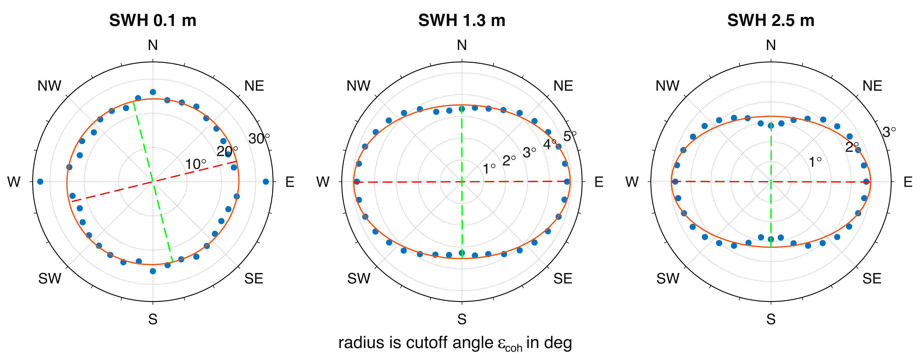
The resulting average correlation lengths were used to calculate the cutoff angle ε_coh from Equation (8) again by application of Newton’s method. Figure 6 depicts the cutoff angles for the different azimuthal directions for SWH values of 0.1 m, 1.3 m, and 2.5 m. The cutoff angles show a clear anisotropic behavior. We estimated the semi-minor and semi-major axes and the azimuth of the semi-major axis of a fitting ellipse from a least-squares adjustment. The difference of the axes’ length for the first ellipse at a SWH of 0.1 m is not significant. Hence, the direction of the semi-major axis defers from the downwind direction. For all $\mathrm{S}\mathrm{W}\mathrm{H}\ge 0.3\mathrm{m}$, the difference of the axes’ length is significant and the semi-major axes coincides with the downwind direction.

The cutoff angle ε_coh can be calculated also for the minimum and maximum correlation length function presented in Figure 5b. As mentioned above, a random value with a standard deviation s of 5 cm was added to the heights of the simulated wave field. This will have a larger influence on the wave fields with smaller SWH values. We took this into account by calculating σ_h in Equation (6) as of

$${\mathsf{\sigma }}_{\mathrm{h}}\approx \sqrt{{(\mathrm{S}\mathrm{W}\mathrm{H}/4)}^2+{\mathrm{s}}^2}$$

(14)

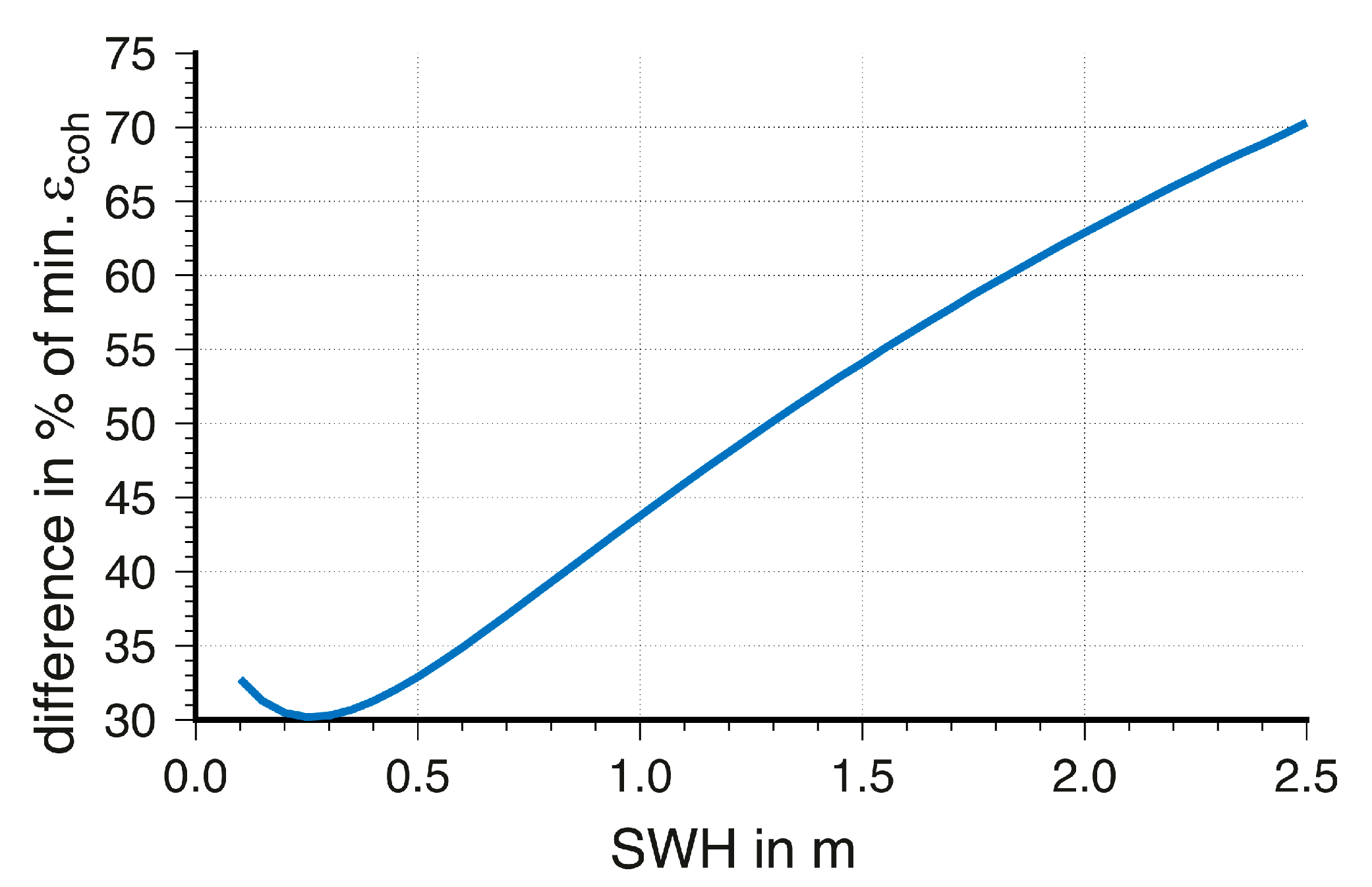
The difference between the maximum and minimum cutoff angle can be related to the minimum cutoff angle. Figure 7 depicts the differences in percent. The differences are more pronounced for increased SWH. This can imply a more significant estimation of the wave direction for higher SWH and explains the discrepancy of the downwind direction and the semi-major axis for a SHW of 0.1 m in Figure 6.

Hence, it appears possible to derive wave directions from the analysis of the anisotropy of the cutoff angles ε_coh. At least for the simulated data, the semi-major axis coincides with downwind direction.

4. Validation with Experimental Data

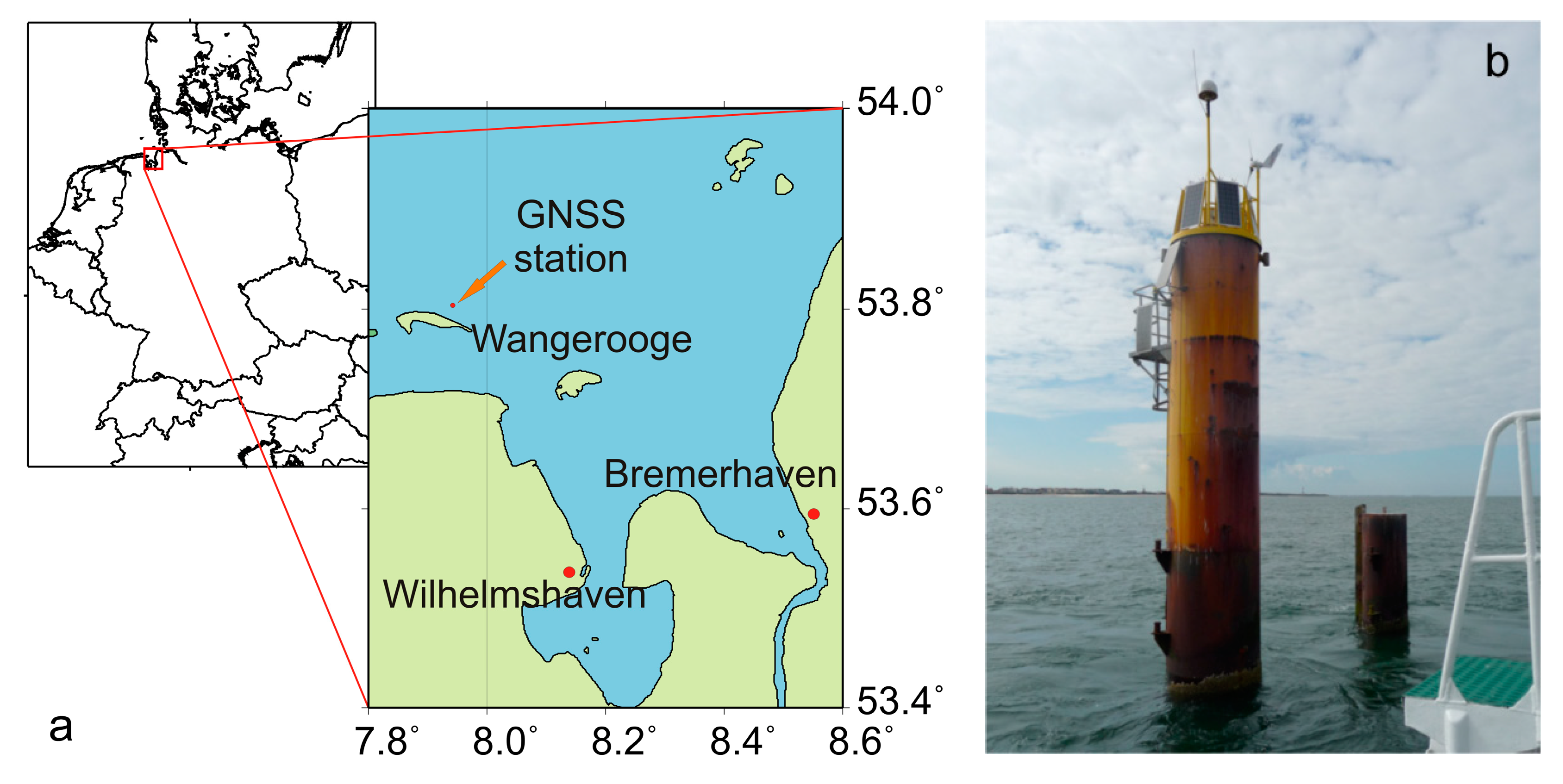
A one-month GNSS data set for validation was collected from a Leica GR10 receiver and a Leica AR25.R3 antenna during July 2018 (day-of-year 185 to 216). This equipment is operated by the German Federal Institute of Hydrology (Bundesanstalt für Gewässerkunde, BfG) and is installed atop of a pile at the tide gauge station TGW2 (Figure 8) approximately 1.7 km north of the coast of the island of Wangerooge in the North Sea. The tide gauge station is approximately 24 km from the wave buoy ElbeWR in the North Sea that was mentioned in Section 3. For purpose of comparison, the SWH observed at the buoy was corrected for the differences between the modeled SWH at the buoy and the tide gauge. The differences were derived from the numerical wave model CWAM (Coupled Wave Current Model) of the German Weather Service (Deutscher Wetterdienst, DWD) [29]. The resulting SWH for the period covered by the GNSS data set is presented in Figure 9 (grey line).

The distance from the APC to tide gauge zero was taken from information provided by BfG. The tide gauge readings with respect to the same tide gauge zero were obtained from freely available data of the German Federal Waterways and Shipping Administration (Wasserstraßen- und Schifffahrtsverwaltung des Bundes, WSV). Hence, the reflector height in Equation (1), ranging between about 10.1 m and 14.4 m, is known at all observation epochs and needs not to be deduced from GNSS SNR data. The GNSS data from GPS and GLONASS were collected at a sample rate of 1 s. Additional weather data were provided by the DWD from the nearby weather station Alte Weser Lighthouse.

The formulation of the trend by a simple low-order polynomial in Equation (1) cannot describe anisotropic effects (i.e., from antenna gain patterns). Hence, the GNSS data for every satellite was split into ascending and descending tracks to prevent systematic errors. Additionally, this splitting allows us to estimate the attenuation for different azimuths covered by the ascending and descending tracks independently, and increase the number of useable cutoff angles. To avoid influences from the shore of the island, only data with elevation angles over 1° were used. The attenuation of the SNR signal of this antenna type shows a strong degradation for elevation angles above about 10° (see Figure 1). Therefore, we restricted the data set for elevation angles below 10°. All elevation angles were corrected for atmospheric refraction and curvature of the reflecting surface as mentioned in Section 2. To allow for a good coverage of the horizon, we binned the data into 3h time slots. Since the evolution of the sea state is a slow process at least for the data set used here (see Figure 9), we assume that this bin size seems to be reasonable. Data sets were assigned to the time slots according to the time of their mid epochs to avoid cutting of data sets overlapping the bound of the time slots. Satellites tracks with elevation ranges of less than 3° were excluded from the analysis.

In total, 252 time slots were analyzed with an average number of about 25 assigned satellite tracks per time slot. The unknown parameters of a polynomial trend function together with the amplitude Amp, the phase offset ${\mathsf{\varphi }}_0$, and the damping coefficient d from Equation (1) were estimated from a least-squares adjustment individually for every satellite involved. We applied the Levenberg–Marquardt algorithm for the non-linear optimization problem to avoid divergence due to possible insufficient initial values for the damping coefficient.

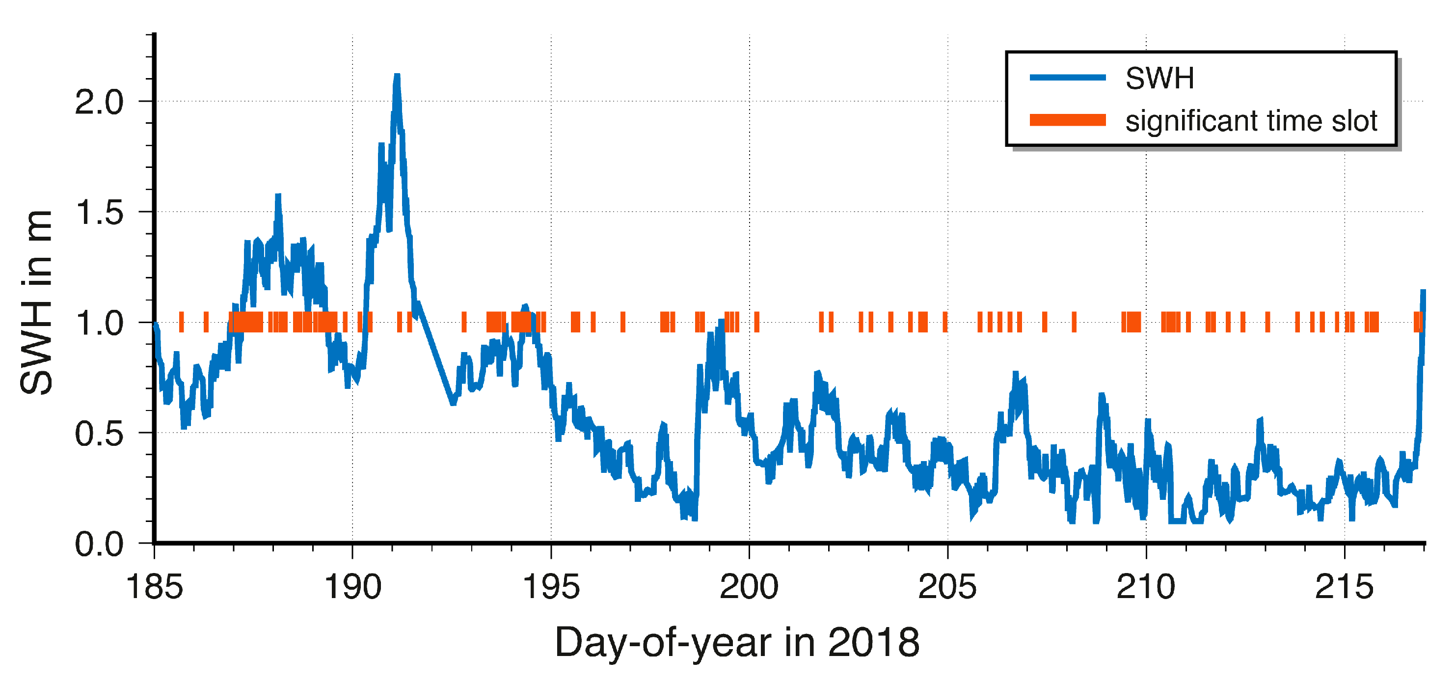
The cutoff angles ε_coh were than calculated according to Equation (5), whereby a factor f of 1.0 was used. Likewise, the standard deviation of the cutoff angles was derived from a covariance propagation of the results from the least-squares adjustment. All resulting cutoff angles together with their corresponding azimuth assigned to the same time slot were then used to fit an ellipse by means of a weighted least-squares adjustment, while the weights were derived from the standard deviation of the cutoff angles. For about 36% of all time slots the adjustment yielded significant differences of the semi-major and semi-minor axes of the ellipses. Figure 9 depicts the SWH at tide gauge together with significant time slots in red (at SHW = 1 m). About 73% of the time slots with significant differences show an average SWH of more than 0.3 m, while about 61% of the time slots with insignificant differences show an average SWH of less than 0.5 m. On day-of-year 191 and 192, the SWH reached values of more than 2 m but only some slots of these days show significant results. This seems to contradict the finding from the simulation in Section 3, that for higher SWH the results will be significant. However, in reality the oscillation of GNSS SNR observations at low elevation angles might become noisier due to shadowing effects or stronger tropospheric refraction. For the case of the tide gauge in the vicinity to the coast of the island, also breaking waves or converted shallow water waves might be included in the data set. An identification of such influence based on the existing data was not possible.

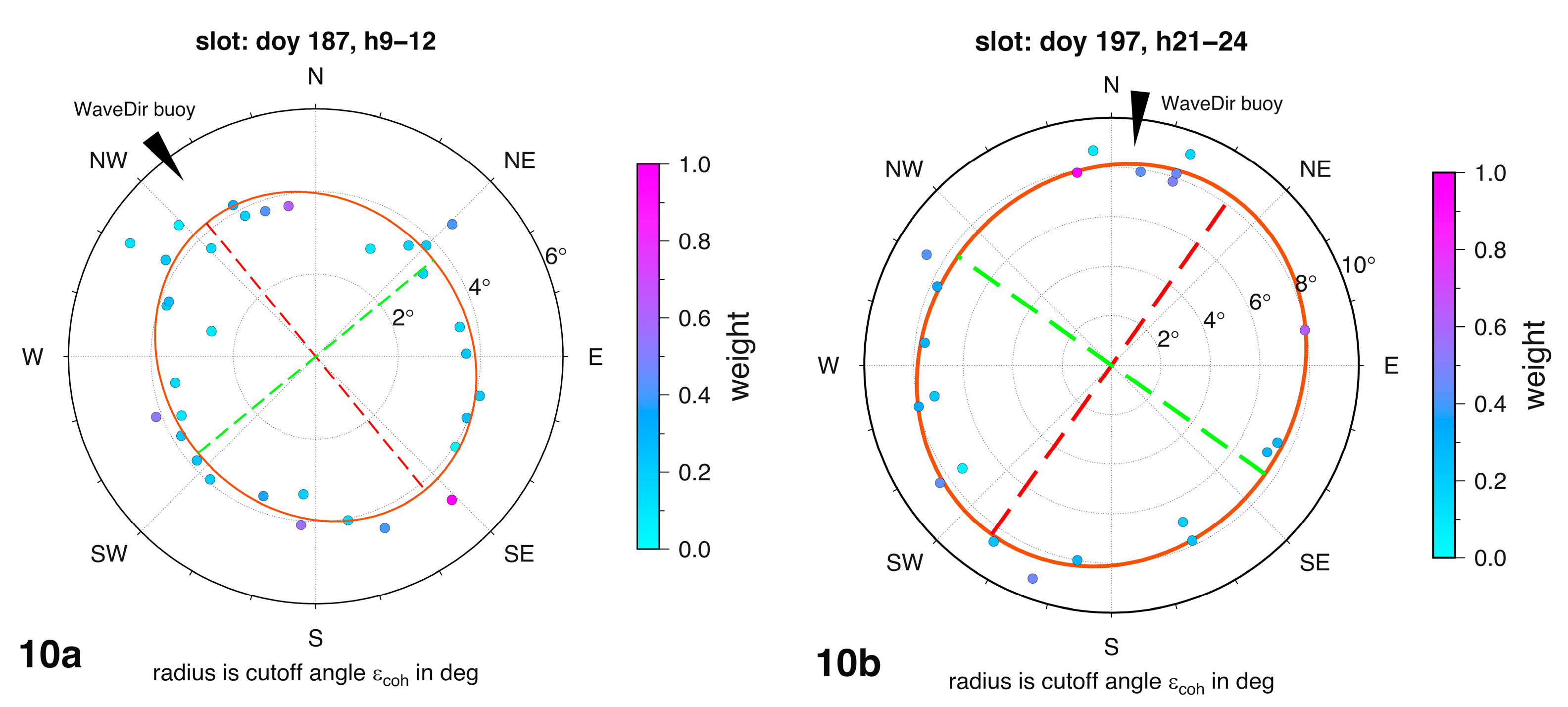
The resulting azimuthal directions of the semi-major axes can be compared to the average wave direction calculated for the time slots from the observations at the wave buoy. It must be mentioned that the directions of the semi-major axes do not allow distinguishing between downwind or upwind direction. Hence, the resulting azimuths are ambiguous by 180°. Figure 10 depicts two typical results for larger and smaller SWH. The black arrow represents the average wave direction at the buoy.

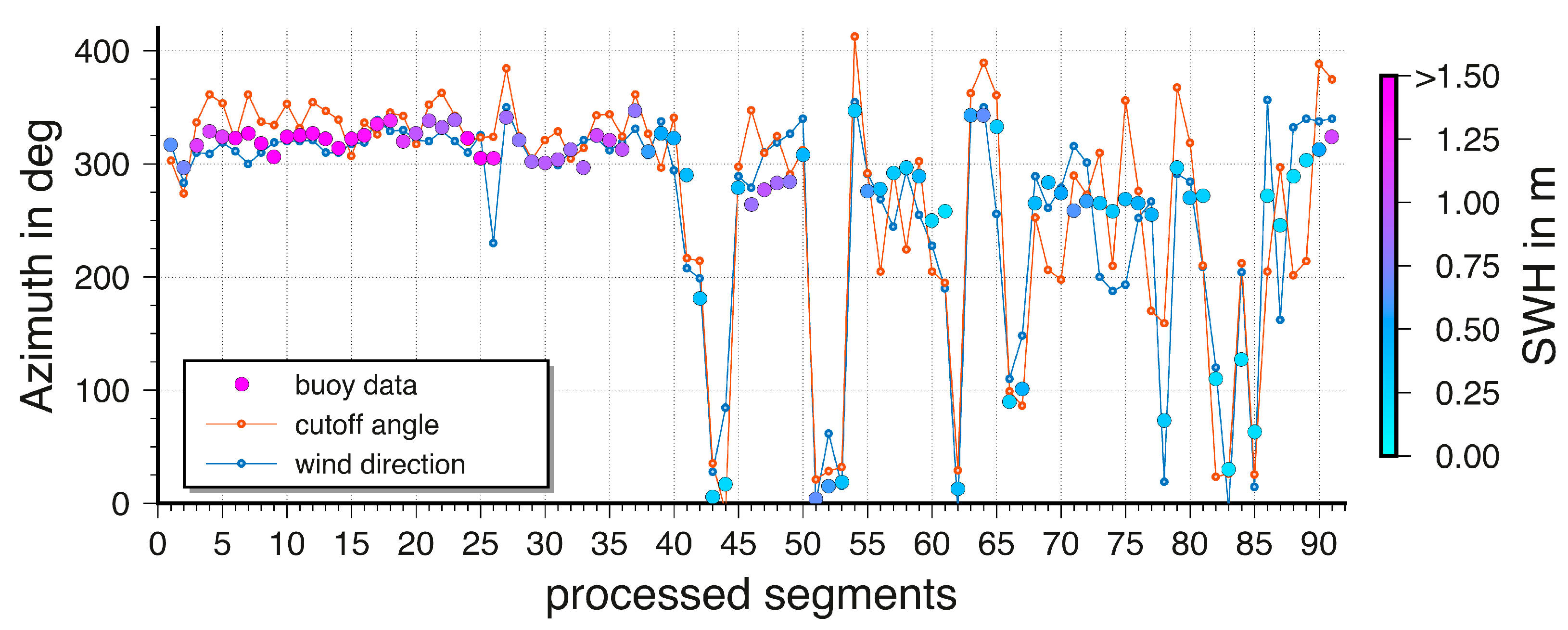
All resulting azimuths were compared to the wave direction from the buoy. The downwind or upwind direction was calculated from the azimuths by adding or subtracting 180° so that the differences to the wave direction from the buoy become minimal. We carried out the same calculation for the wind direction that was taken from the mentioned weather data at the Alte Weser Lighthouse. Figure 11 depicts a comparison of the data sets for all significant segments. In particular, for larger SWH the similarity of the results from the analysis of the cutoff angle and the wave direction from the buoy is obvious. It should be pointed out here, that the wave directions from the buoy show a spreading between 20° and 80°, depending on the SWH as mentioned in Section 3. Unfortunately, the uncertainties for the wind direction and the wave direction from the buoy data were not provided. We calculated the formal standard deviation for the wave directions derived from cutoff angles as 0.22° on average with a minimum of 0.09° and a maximum of 3.54°.

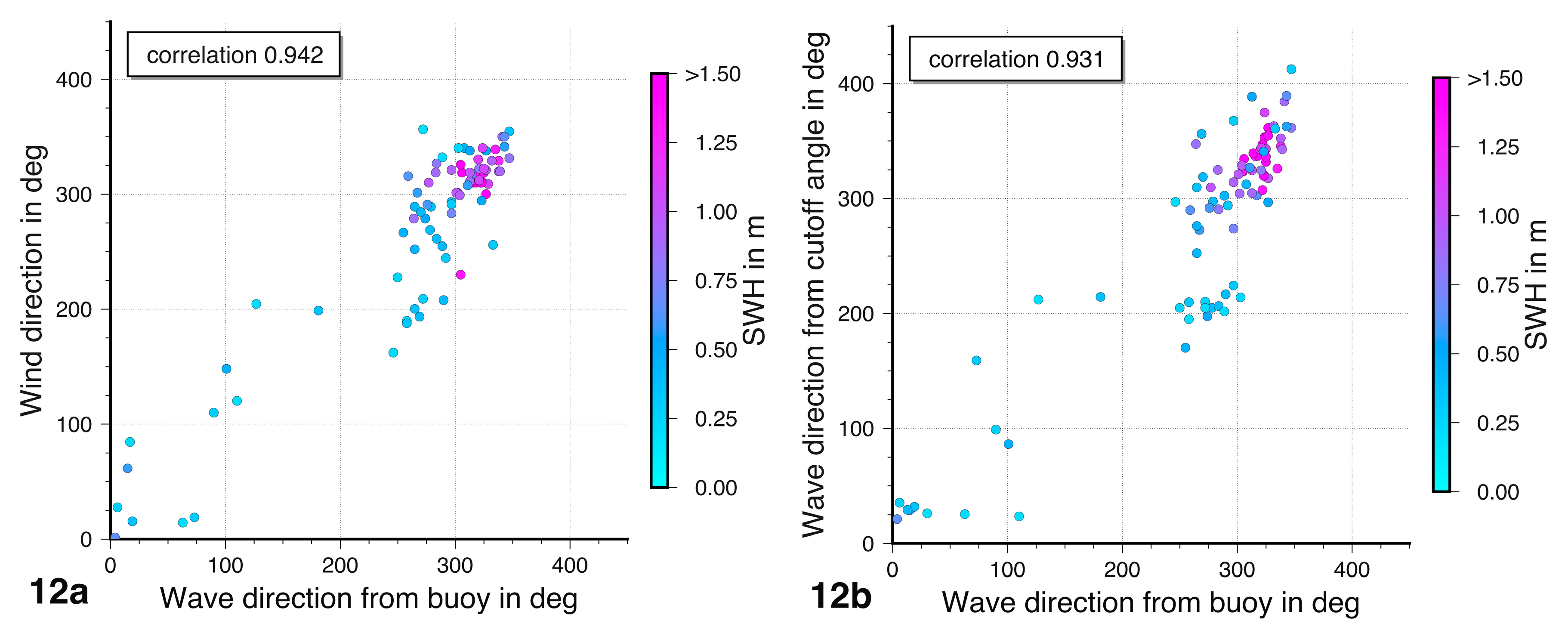
The good agreement of the directions is emphasized by the high correlation between the data sets presented in Figure 12. The correlation coefficient between the wave direction from the buoy and the wind direction is about 0.94, while for the wave direction from the cutoff angles it reaches 0.93. It is remarkable that in both data plots a cluster of off-correlation values at a wave direction of about 290° occur. That indicates a possible discrepancy between the wave directions observed at the buoy and at the tide gauge position. This discrepancy is not related to a specific SWH or wave direction. Unfortunately, the reason for the misfit cannot be verified based on this data set.

5. Conclusions and Discussion

Besides its roughness, the correlation length of a sea surface is of major importance in the analysis of the interference pattern of GNSS SNR data. In general, higher SWH values yield a larger correlation length which results in an increase of the incoherent part of the mean scattered power from a reflecting water surface. Hence, the cutoff angles, the elevation angles at which the coherence is lost, become smaller with increased correlation length.

It is reasonable to assume that the correlation length of the waves of water surfaces depend on the direction of the line of sight. For directions that tend to the cross-wind direction the correlation length will be longer than for directions close to a downwind or upwind direction. Therefore, it should be possible to notice the variation in the correlation length likewise in the variation of cutoff angles. In reverse, it should be possible to derive the wave directions from the variation of the cutoff angles if the variation of the correlation length is sufficiently large

It was shown in this work that for simulated but realistic directional wave fields the correlation length varies strongly with the azimuth relative to the wave direction. Calculating the cutoff angles under consideration of the anisotropy of the correlation length and estimating a fitted ellipse allows the wave direction to be derived from the azimuth of the semi-major axis. For smaller SWH the differences of the semi-major and semi-minor axes might become insignificant, yielding incorrect wave directions. For larger SWH these differences will at least theoretically be significant.

The findings from the simulations were verified and largely confirmed by the analysis of data from a GNSS station in the North Sea. For significant results, the correlation to the wave direction observed by a buoy is high and on the same level as the correlation between the wind direction and the wave direction. The significance of the results might be improved if a reliable and automated detection of corrupted data would be applicable.

It should be mentioned that the estimation of the cutoff elevation angle cannot be done for a single epoch because SNR data from a larger part of a satellite track is necessary for a reliable adjustment. The average duration of a satellite track used here is about 20–30 min with a maximum of about one hour. The average variation of the azimuth during this time is about 5–7°, with a maximum of about 20°. This might result in a smearing effect that cannot be avoided when using SNR data. However, the cutoff elevation angle is related to the average azimuth of a satellite track.

For the estimation of the angle of the semi-major axis of the ellipse from the anisotropy of the cuttoff elevation angles, the water surface must be covered by some specular points in different azimuths. Therefore, the method demonstrated here can be applied best at sites with a 360-degree view to the water surface. Restricted stations with a smaller view angle can also yield reasonable wave directions but the results might become less precise due to geometric reasons. For stations where only specular points from a small portion of the horizon can be used, the application of the method presented here is not recommended unless a reasonable number of specular points could be used. The data used in this investigation contain GPS and GLONASS observations only. Data from additional satellite systems would increase the number of specular points. If many satellites are visible and usable in different azimuths at the same time, a near-real-time estimation of wave directions might be possible.

Even if only some sites might be used in a post-processing mode, the number of available wave direction observations would be increased. Hence, besides the estimation of water surface heights and SWH, GNSS reflectometry might yield another important benefit for coastal zone management.

References

- Martin-Neira, M.A. A Passive Reflectometry and Interferometry System (PARIS): Application to ocean altimetry. ESA J. 1973, 17, 331–355. [Google Scholar]
- Clarizia, M.P.; Ruf, C.; Cipollini, P.; Zuffada, C. First spaceborne observation of sea surface height using GPS-Reflectometry. Geophys. Res. Lett. 2016, 43, 767–774. [Google Scholar] [CrossRef]
- Larson, K.M.; Small, E.E.; Gutmann, E.; Bilich, A.; Axelrad, P.; Braun, J. Using GPS multipath to measure soil moisture fluctuations: Initial results. GPS Solut. 2008, 12, 173–177. [Google Scholar] [CrossRef]
- Larson, K.M.; Gutmann, E.D.; Zavorotny, V.U.; Braun, J.J.; Williams, M.W.; Nievinski, F.G. Can we measure snow depth with GPS receivers? Geophys. Res. Lett. 2009, 36, 3171. [Google Scholar] [CrossRef]
- Larson, K.M.; Löfgren, J.S.; Haas, R. Coastal sea level measurements using a single geodetic GPS receiver. Adv. Space Res. 2013, 51, 1301–1310. [Google Scholar] [CrossRef]
- Roggenbuck, O.; Reinking, J. Sea Surface Heights Retrieval from Ship-Based Measurements Assisted by GNSS Signal Reflections. Mar. Geod. 2019, 42, 1–24. [Google Scholar] [CrossRef]
- Wang, N.; Xu, T.; Gao, F.; Xu, G. Sea Level Estimation Based on GNSS Dual-Frequency Carrier Phase Linear Combinations and SNR. Remote Sens. 2018, 10, 470. [Google Scholar] [CrossRef]
- Bishop, G.J.; Klobuchar, J.A.; Doherty, P.H. Multipath effects on the determination of absolute ionospheric time delay from GPS signals. Radio Sci. 1985, 20, 388–396. [Google Scholar] [CrossRef]
- Georgiadou, P.Y.; Kleusberg, A. On carrier signal multipath effects in relative GPS positioning. Manuscr. Geod. 1988, 13, 172–179. [Google Scholar]
- Nievinski, F.G.; Larson, K.M. Forward modeling of GPS multipath for near-surface reflectometry and positioning applications. GPS Solut. 2014, 18, 309–322. [Google Scholar] [CrossRef]
- Alonso-Arroyo, A.; Camps, A.; Park, H.; Pascual, D.; Onrubia, R.; Martin, F. Retrieval of Significant Wave Height and Mean Sea Surface Level Using the GNSS-R Interference Pattern Technique: Results From a Three-Month Field Campaign. IEEE Trans. Geosci. Remote Sens. 2015, 53, 3198–3209. [Google Scholar] [CrossRef]
- Brummel, F.; Roggenbuck, O.; Reinking, J. Estimation of significant wave heights using GNSS-SNR data from moving ships. In EGU General Assembly Conference Abstracts; EGU 2018: Vienna, Austria, 2018; p. 14260. [Google Scholar]
- Roggenbuck, O.; Reinking, J.; Lambertus, T. Determination of Significant Wave Heights Using Damping Coefficients of Attenuated GNSS SNR Data from Static and Kinematic Observations. Remote Sens. 2019, 11, 409. [Google Scholar] [CrossRef]
- Beckmann, P.; Spizzichino, A. The Scattering of Electromagnetic Waves from Rough Surfaces; Artech House: Norwood, MA, USA, 1987; ISBN 0890062382. [Google Scholar]
- Semmling, A.M.; Leister, V.; Saynisch, J.; Zus, F.; Heise, S.; Wickert, J. A Phase-Altimetric Simulator: Studying the Sensitivity of Earth-Reflected GNSS Signals to Ocean Topography. IEEE Trans. Geosci. Remote Sens. 2016, 54, 6791–6802. [Google Scholar] [CrossRef]
- Bennett, G.G. The Calculation of Astronomical Refraction in Marine Navigation. J. Navig. 1982, 35, 255. [Google Scholar] [CrossRef]
- Santamaría-Gómez, A.; Watson, C.; Gravelle, M.; King, M.; Wöppelmann, G. Levelling co-located GNSS and tide gauge stations using GNSS reflectometry. J. Geod. 2015, 89, 241–258. [Google Scholar] [CrossRef]
- Santamaria-Gomez, A.; Watson, C. Remote leveling of tide gauges using GNSS reflectometry: Case study at Spring Bay, Australia. GPS Solut. 2017, 21, 451–459. [Google Scholar] [CrossRef]
- Williams, S.D.P.; Nievinski, F.G. Tropospheric delays in ground-based GNSS multipath reflectometry-Experimental evidence from coastal sites. J. Geophys. Res. Solid Earth 2017, 122, 2310–2327. [Google Scholar] [CrossRef]
- Reinking, J. GNSS-SNR water level estimation using global optimization based on interval analysis. J. Geod. Sci. 2016, 6, 497. [Google Scholar] [CrossRef]
- Nayar, S.K.; Ikeuchi, K.; Kanade, T. Surface reflection: Physical and geometrical perspectives. IEEE Trans. Pattern Anal. Mach. Intell. 1991, 13, 611–634. [Google Scholar] [CrossRef]
- DNV. Environmental Conditions and Environmental Loads. Det Norske Veritas, Recommend Practice. DNV-RP-C205. Available online: https://rules.dnvgl.com/docs/pdf/DNV/codes/docs/2014-04/RP-C205.pdf (accessed on 18 March 2019).
- Guo, Q.Y.; Xu, Z.Y.; Sun, Y.J. Three-Dimensional Ocean Wave Simulation Based on Directional Spectrum. AMM 2011, 94–96, 2074–2079. [Google Scholar] [CrossRef]
- Tessendorf, J. Simulating Ocean Water. In Proceedings of the 26th International Conference and Exhibition on Computer Graphics and Interactive Techniques (SIGGRAPH 1999), Los Angeles, CA, USA, 8–13 August 1999; Course Notes 26. Available online: http://citeseerx.ist.psu.edu/viewdoc/download?doi=10.1.1.161.9102&rep=rep1&type=pdf (accessed on 18 March 2019).
- Fréchot, J. Realistic Simulation of Ocean Surface Using Wave Spectra. In Proceedings of the GRAPP 2006-Proceedings of the 1st International Conference on Computer Graphics Theory and Applications, Setúbal, Portugal, 25–28 February 2006. [Google Scholar]
- Hasselmann, K.; Barnett, T.P.; Bouws, E.; Carlson, H.; Cartwright, D.E.; Enke, K.; Ewing, J.A.; Gienapp, H.; Hasselmann, D.E.; Kruseman, P.; et al. Measurements of Wind-Wave Growth and Swell Decay during the Joint North Sea Wave Project (JONSWAP); Deutches Hydrographisches Institut: Hamburg, Gemany, 1973; Reihe A (8), Nr. 12. [Google Scholar]
- Pierson, W.J.; Moskowitz, L. A proposed spectral form for fully developed wind seas based on the similarity theory of S. A. Kitaigorodskii. J. Geophys. Res. 1964, 69, 5181–5190. [Google Scholar] [CrossRef]
- Boer, J.G.D. On the Correlation Functions in Time and Space of Wind-Generated Ocean Waves; SACLANT ASW Research Centre: La Spezia, Italy, 1969. [Google Scholar]
- Kieser, J.; Bruns, T.; Lindenthal, A.; Brüning, T.; Janssen, F.; Behrens, A.; Li, X.; Lehner, S.; Pleskachevsky, A. First Studies with the High-Resolution Coupled Wave Current Model CWAM and other Aspects of the Project Sea State Monitor. In Proceedings of the 13th International Workshop on Wave Hindcasting and 4th Coastal Hazard Symposium, Banff, AB, Canada, 27 October–1 November 2013; Available online: http://www.waveworkshop.org/13thWaves/Papers/cwam_article_kieser_et_al.pdf (accessed on 18 March 2019).
Figure 1.
Detrended signal-to-ratio (SNR) data from a global navigation satellite systems (GNSS) receiver at a tide gauge station (grey dots) forday-of-year 190 in 2018, GPS PRN 8. The red line shows the adjusted oscillation, the horizontal continuous blue lines show the threshold according to Equation (4) for the factor f, and the vertical dashed blue lines present the corresponding cutoff angle εcoh with 7.52° for f = 0.5 and 6.06° for f = 1.0.
Figure 2.
Cutoff angle εcoh as a function of different correlation lengths T and significant wave heights (SWH). The cutoff angle was derived for incoh = 1.
Figure 3.
Observed peak period (a) and directional spreading (b) plotted over SWH for the wave buoy ElbeWR. Red lines show the functions used to derive Tp and and for simulations.
Figure 4.
Simulated wave field for SWH = 2.5 m.
Figure 5.
Correlation lengths for 100 simulated wave fields for a SWH of 2.5 (a). The red line shows the average correlation length for the corresponding azimuth. Minimum and maximum of the mean correlation length for the specific SWH and their quadratic fit (b).
Figure 6.
Cutoff angles for three SWH values and different azimuth (blue dots). Ellipses in red present the least-squares fit with their semi-major (red line) and semi-minor (green line) axes. The axes at SHW of 0.1 m do not show a significant difference. All other semi-major axes coincide with the west-to-east downwind direction.
Figure 7.
Differences of the maximum and minimum cutoff angles in relation to the minimum cutoff angle plotted over SWH. The difference is becoming larger and more pronounced with increasing SWH values.
Figure 8.
Position of GNSS station north of the island of Wangerooge (a) and GNSS antenna installed atop of the tide gauge station TGW2 in the North (b) (photo BfG).
Figure 9.
SWH at tide gauge (grey) and significant time slots (red).
Figure 10.
Cutoff angles (grey dots, shading with respect to their weights), adjusted ellipses, and average wave directions derived from buoy data, (a) SWH = 1.2 m, (b) SWH = 0.35 m.
Figure 11.
Wave direction from the buoy (grey dots, shading with respect to SWH), azimuth of semi-major axis derived from the analysis of the cutoff angles (red) and wind direction (blue).
Figure 12.
Correlation between the wave direction from the buoy and the wind direction (a) and the wave direction from the buoy and the wave direction from the cutoff angles (b). The shading of the dots is with respect to SWH.
© 2019 by the authors. Licensee MDPI, Basel, Switzerland. This article is an open access article distributed under the terms and conditions of the Creative Commons Attribution (CC BY) license (http://creativecommons.org/licenses/by/4.0/).