Automated Extraction of Consistent Time-Variable Water Surfaces of Lakes and Reservoirs Based on Landsat and Sentinel-2


Abstract
1. Introduction
2. Data
2.1. Satellite Imagery
2.1.1. Landsat
2.1.2. Sentinel-2
2.2. In Situ Data
2.3. Satellite Altimetry
3. Methodology
3.1. Initialization
3.2. Computation of Monthly Land-Water Masks with Data Gaps
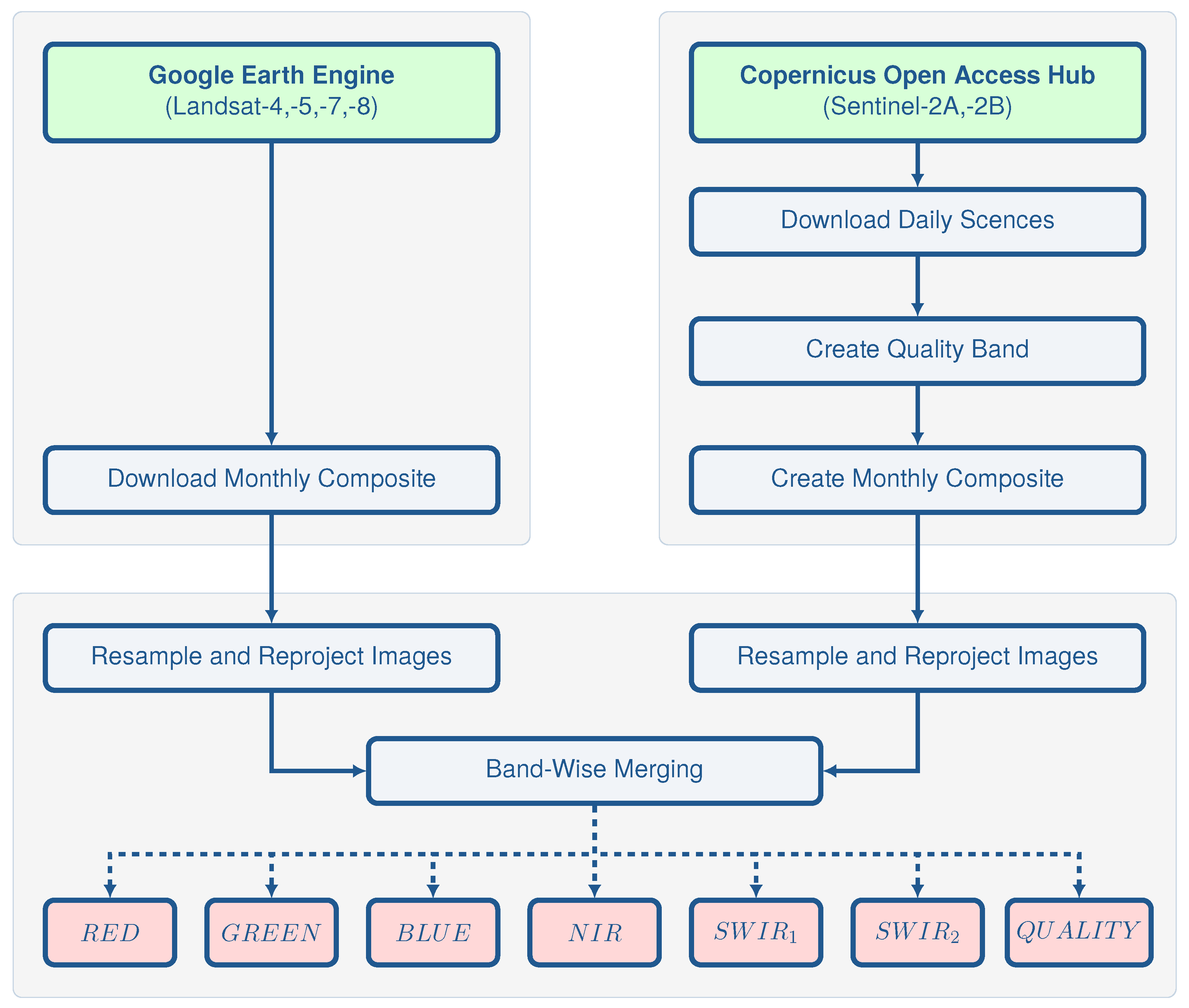
3.2.1. Pre-Processing
Acquisition and Pre-Processing of Landsat Imagery
Acquisition and Pre-Processing of Sentinel-2 Imagery
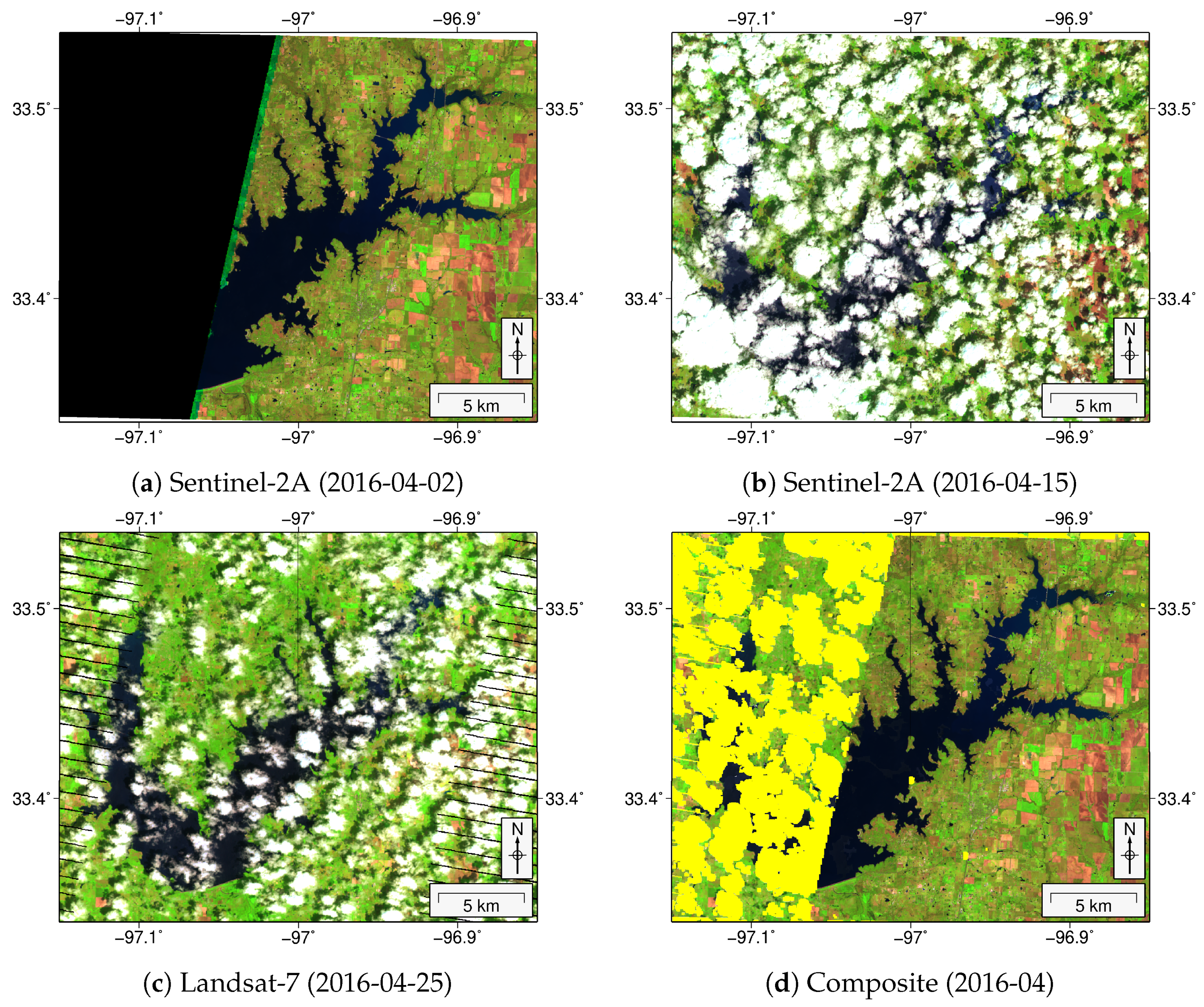
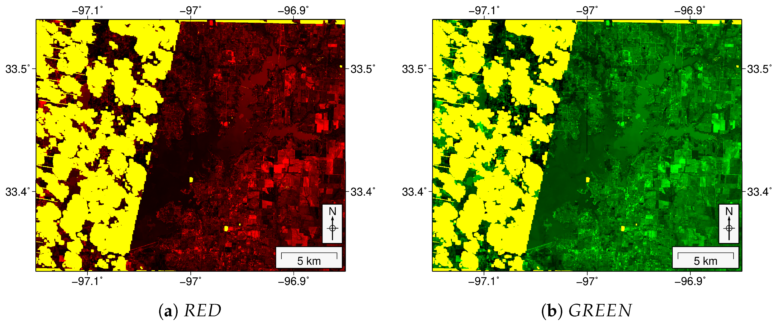
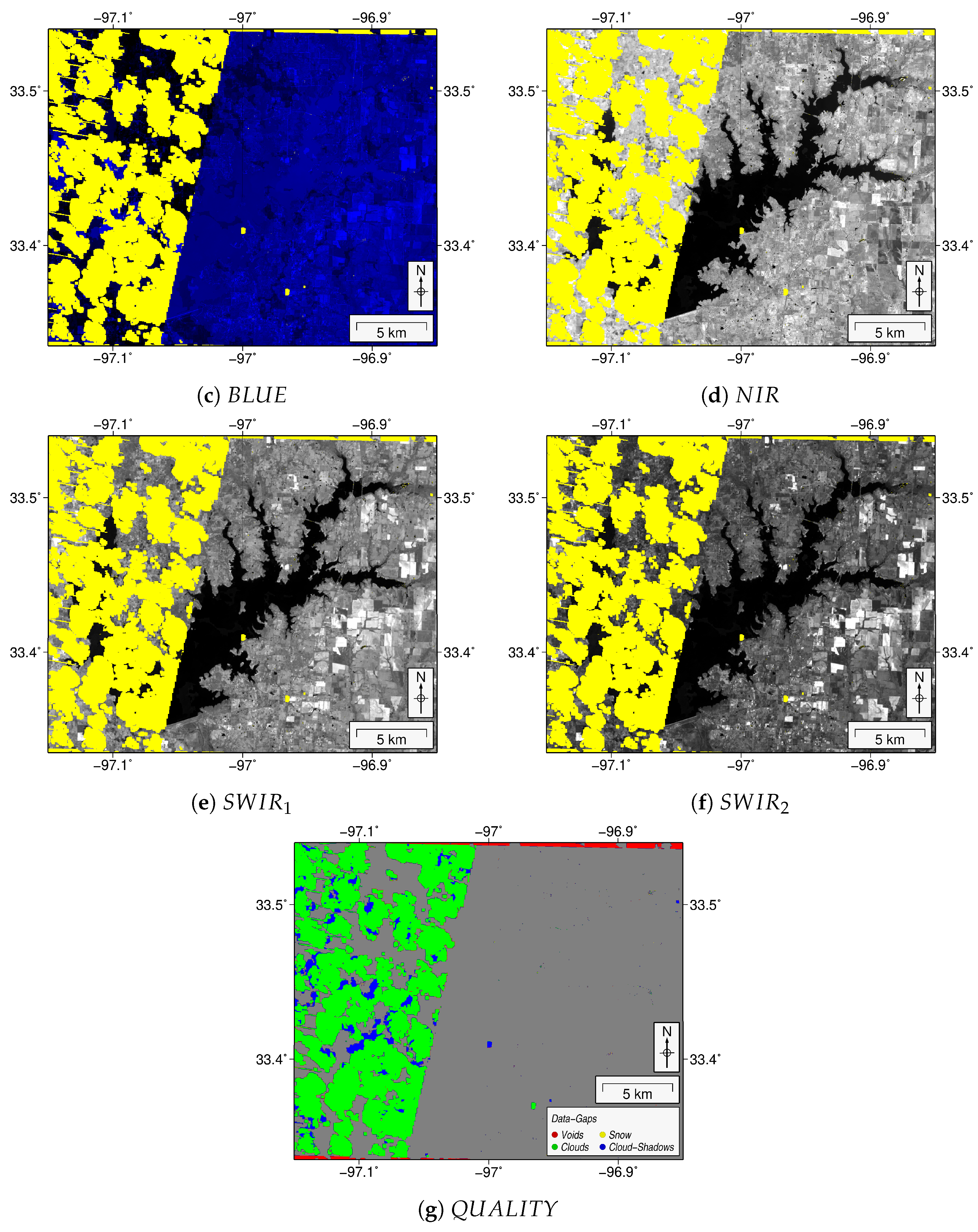
Combination of Landsat and Sentinel-2 Imagery
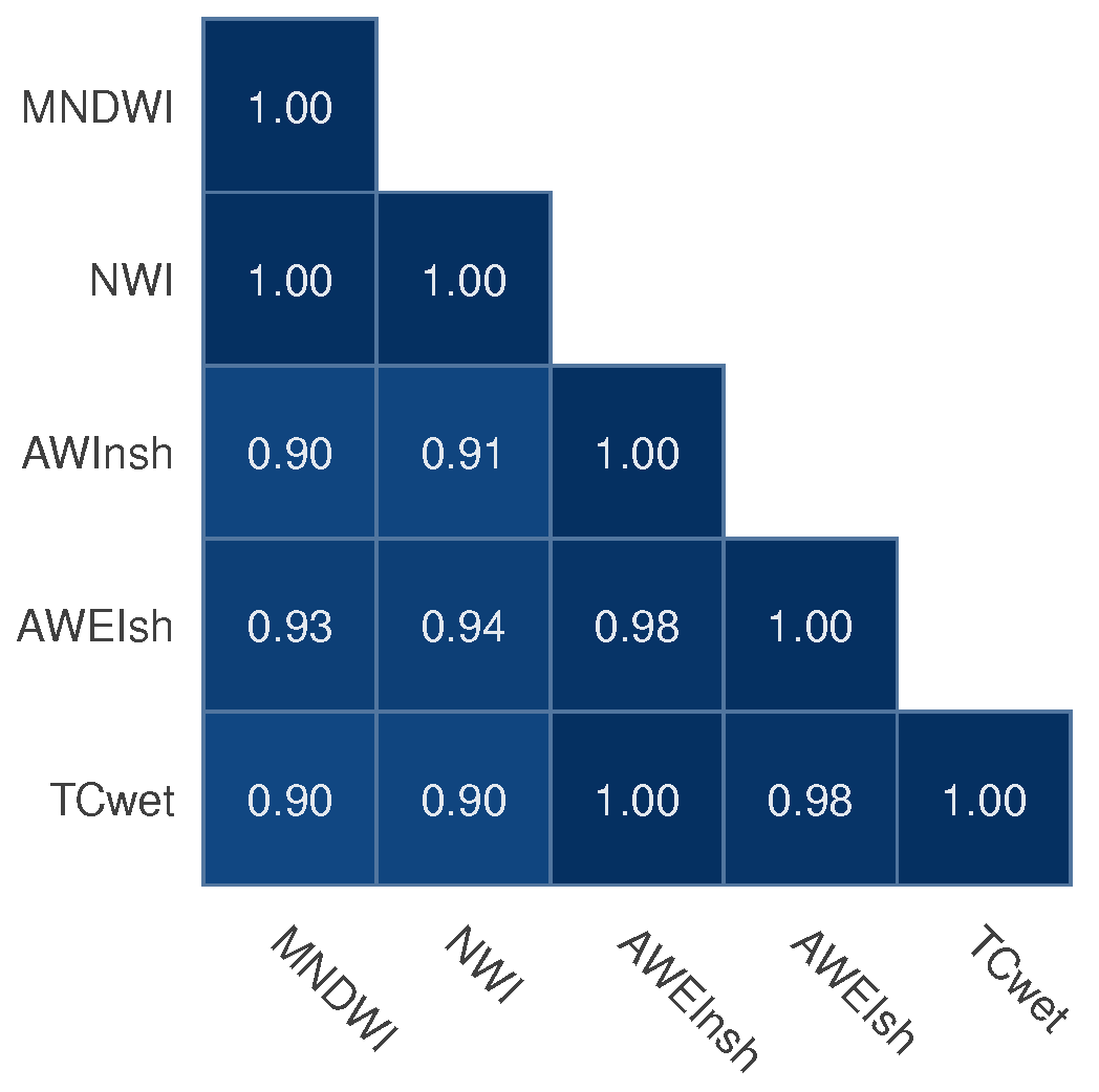
3.2.2. Calculation of Water Indexes
Modified Normalized Difference Water Index (MNDWI)
New Water Index (NWI)
Automated Water Extraction Index for Non-Shadow Areas (AWEInsh)
Automated Water Extraction Index for Shadow Areas (AWEIsh)
Tasseled Cap for Wetness (TCwet)
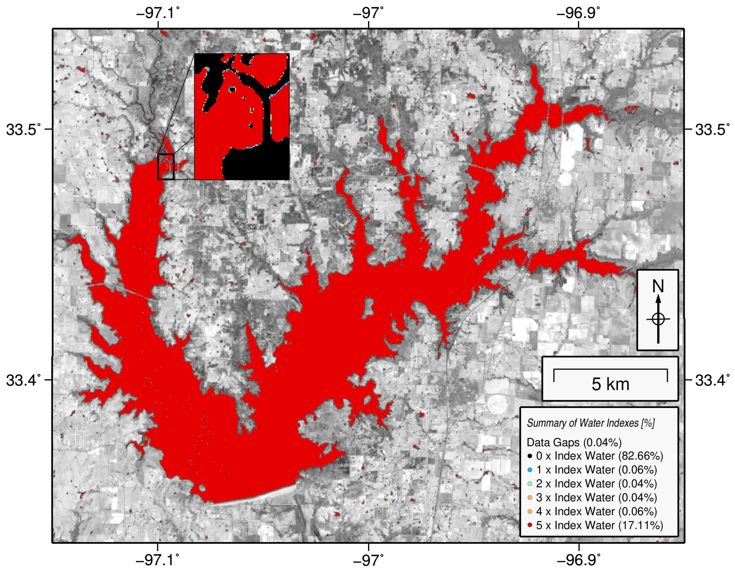
3.2.3. Thresholding
3.2.4. Masking
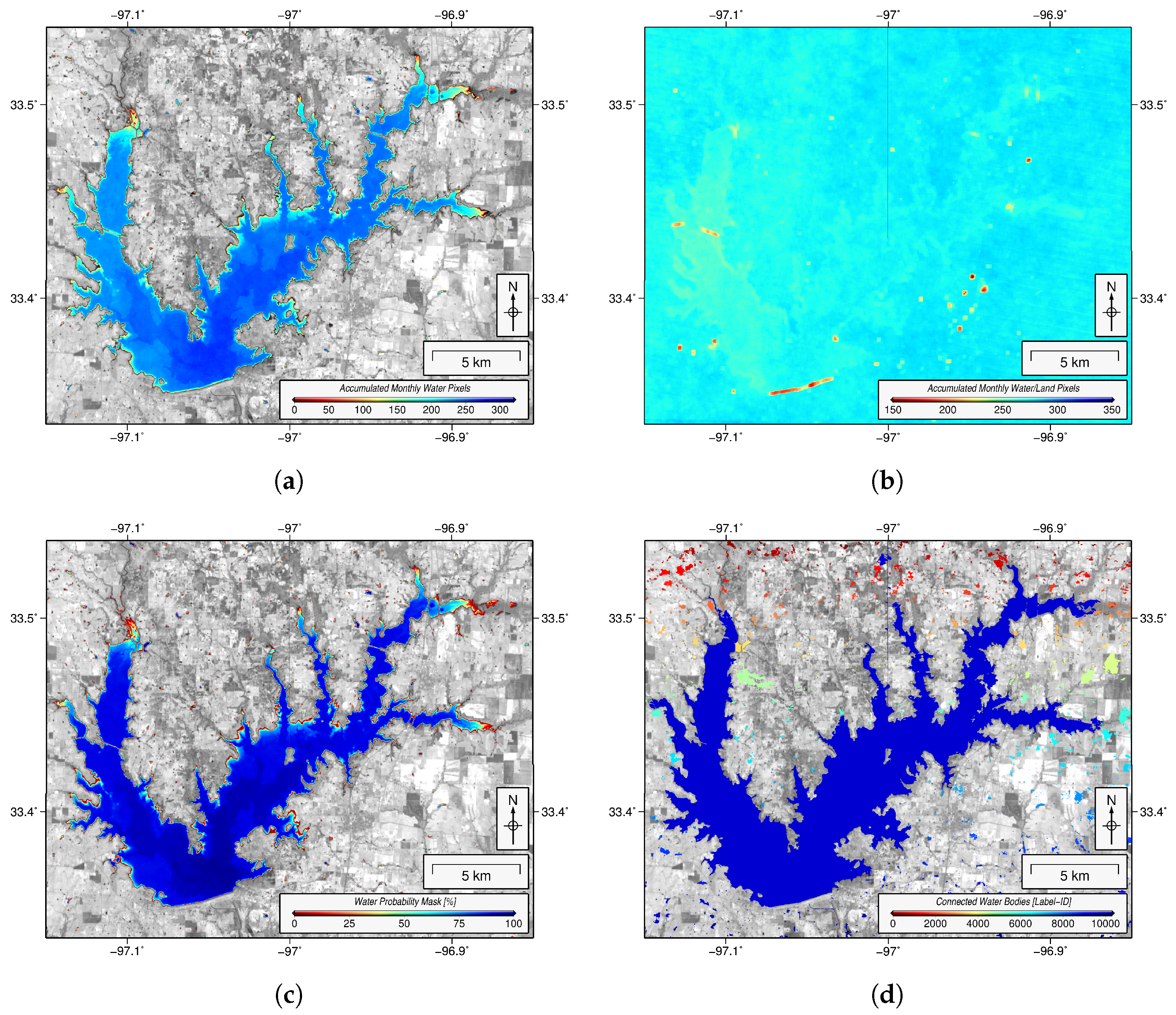
3.3. Calculation of a Long-Term Water Probability Mask
3.4. Filling Data Gaps of Monthly Land-Water Mask
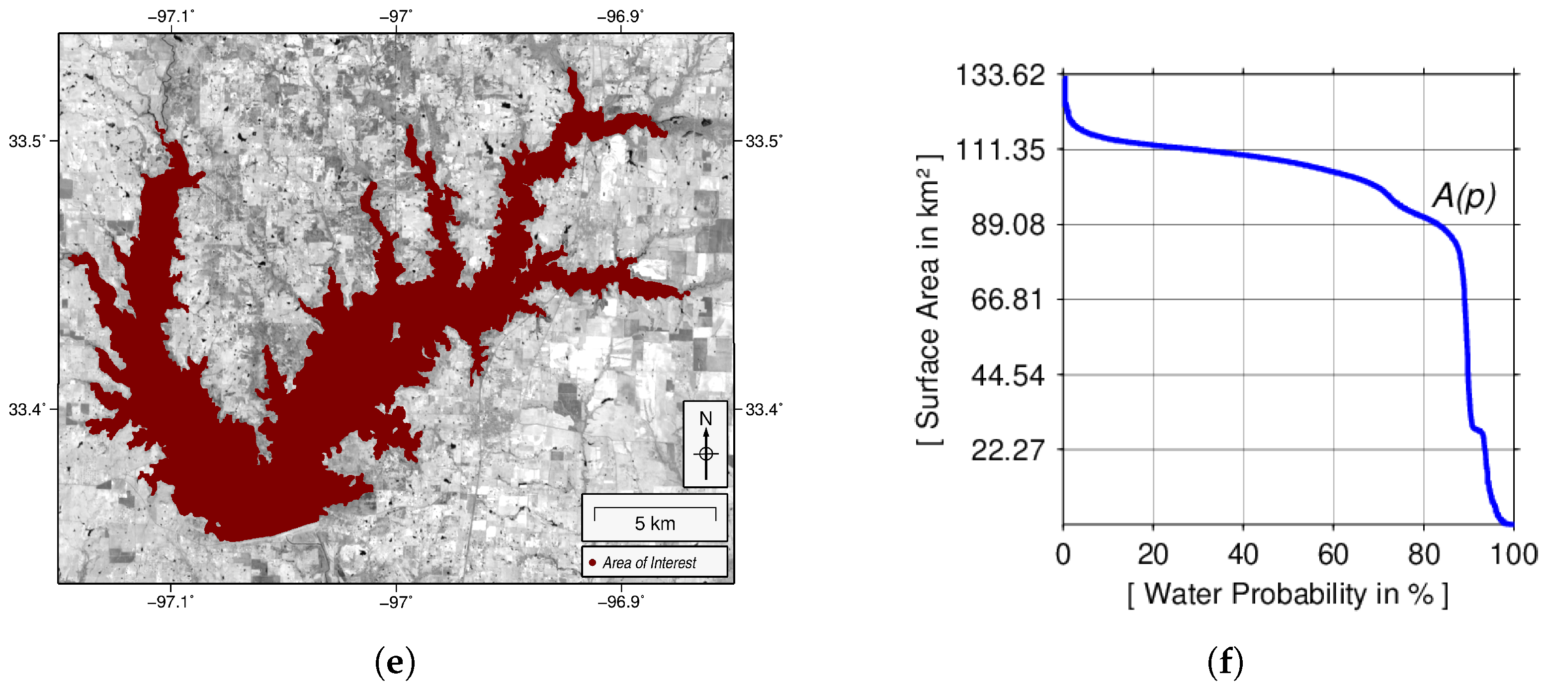
3.5. Computation of Surface Area Time Series
4. Results and Validation
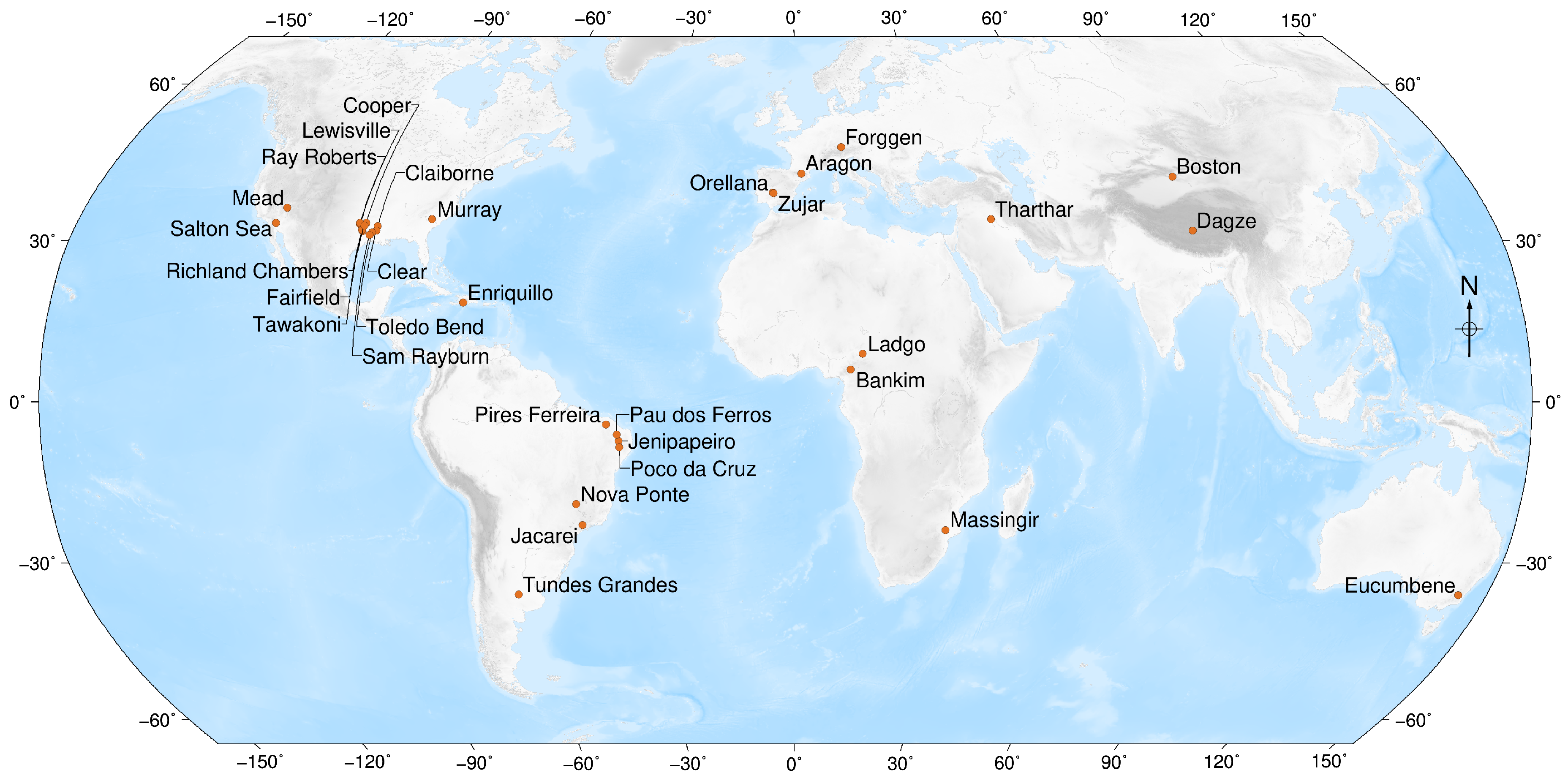
4.1. Study Areas
4.2. Selected Results
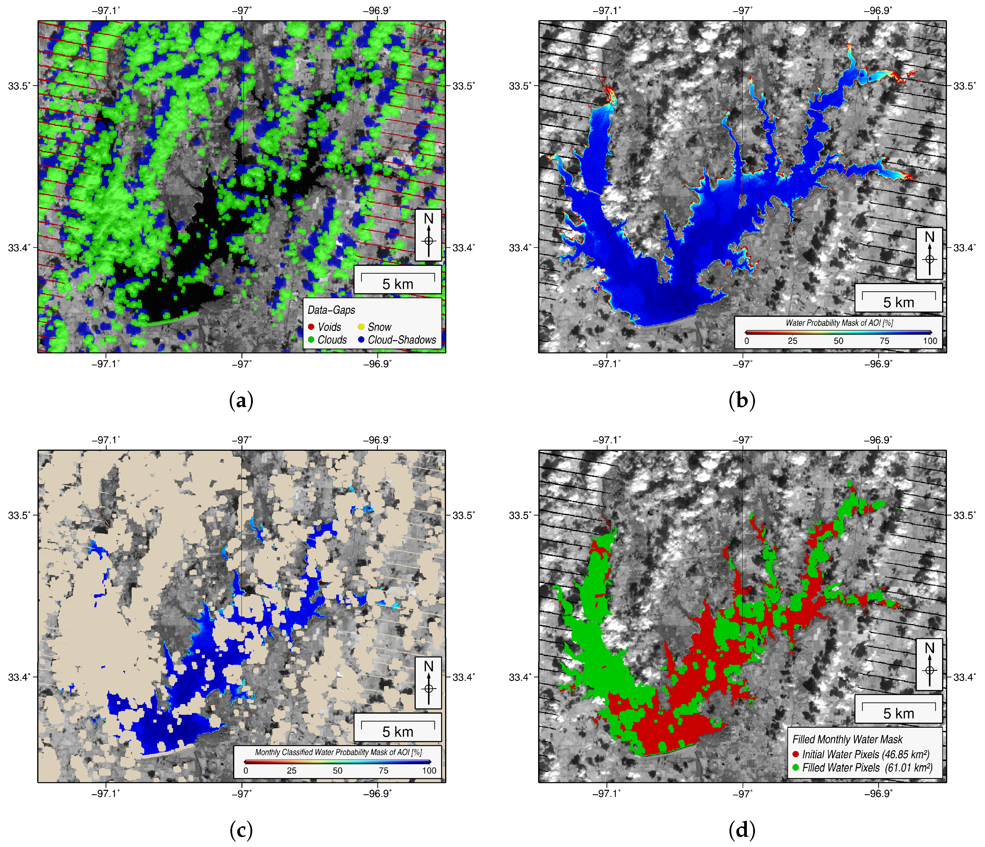
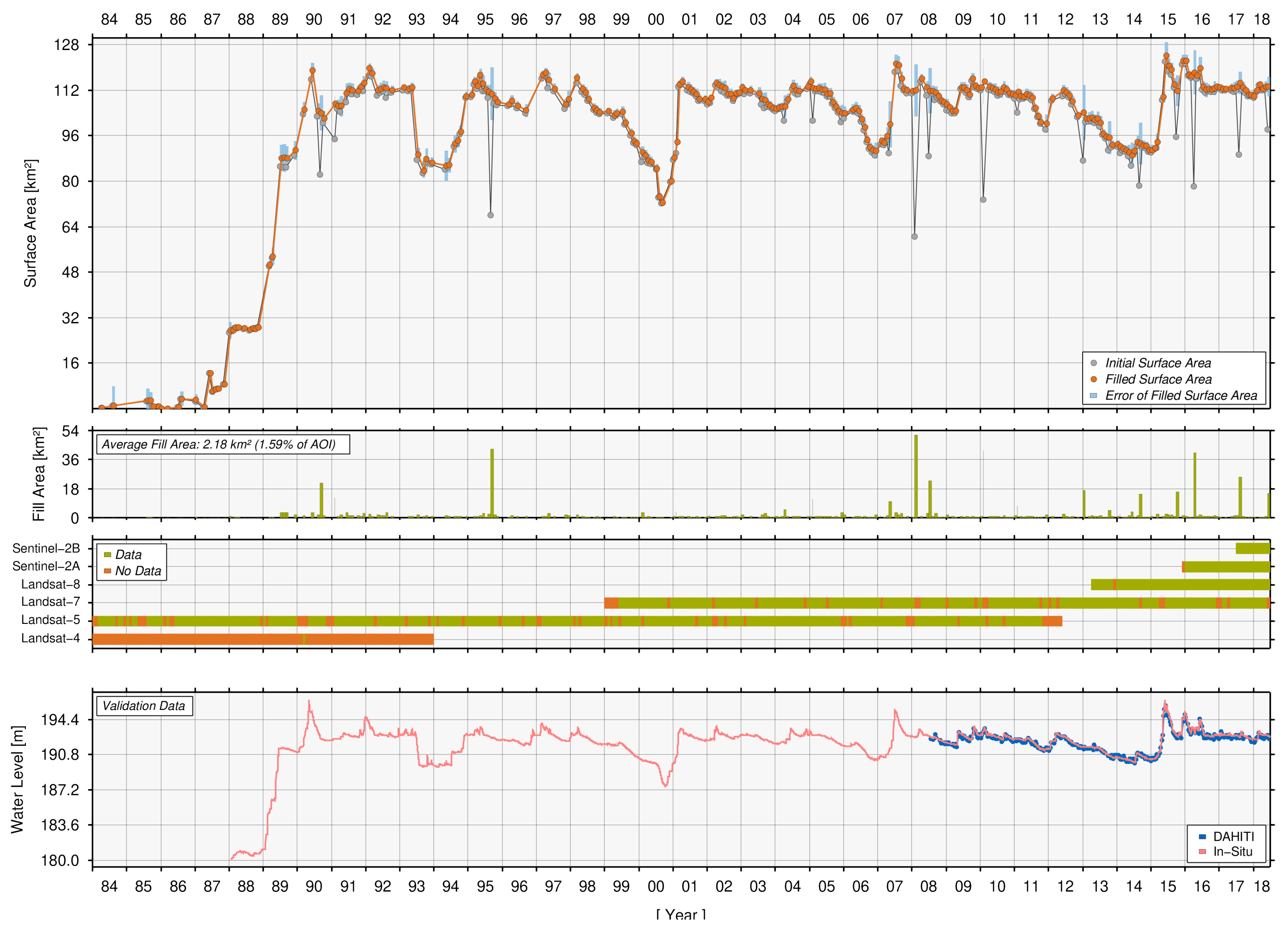
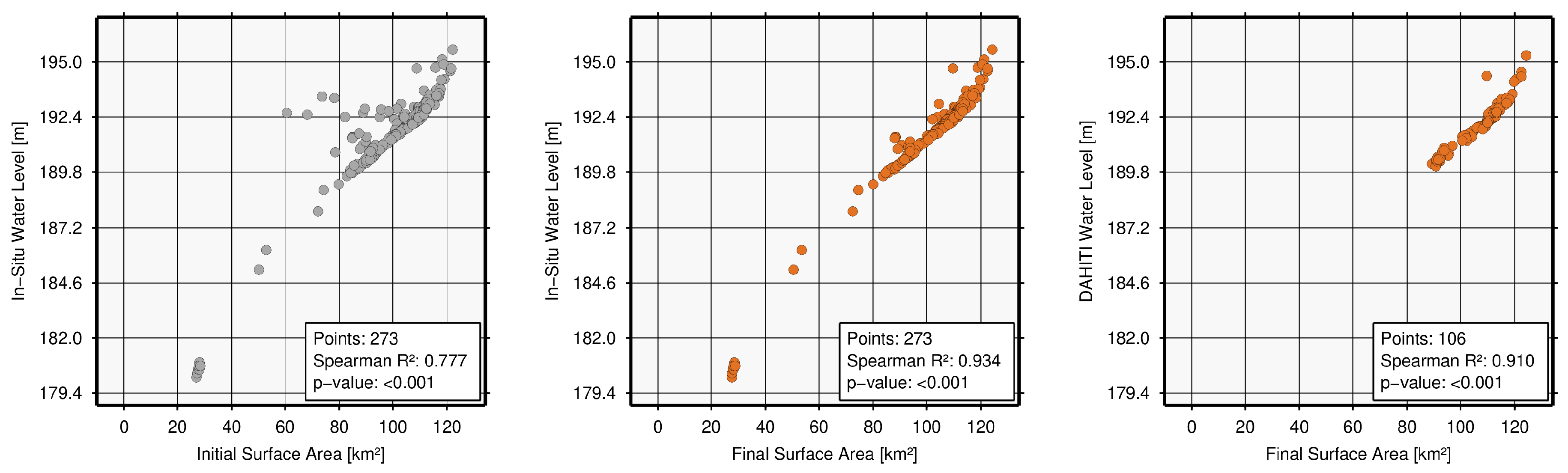
4.2.1. Ray Roberts, Lake
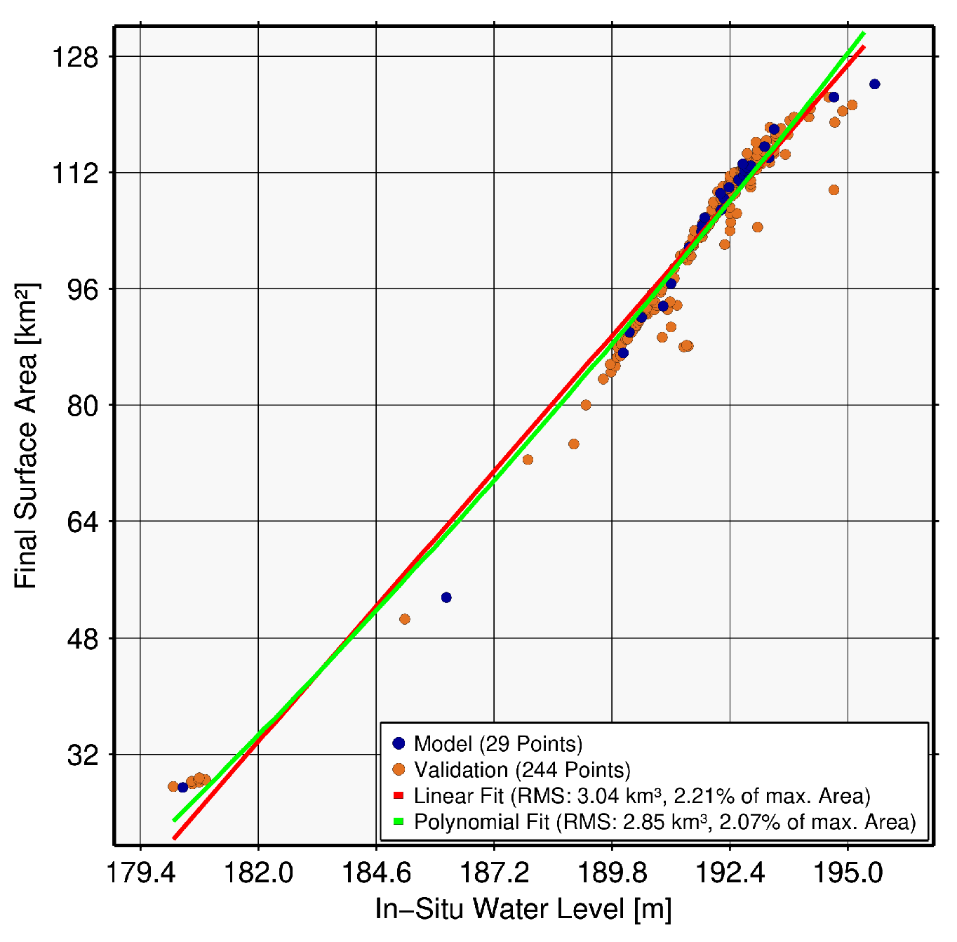
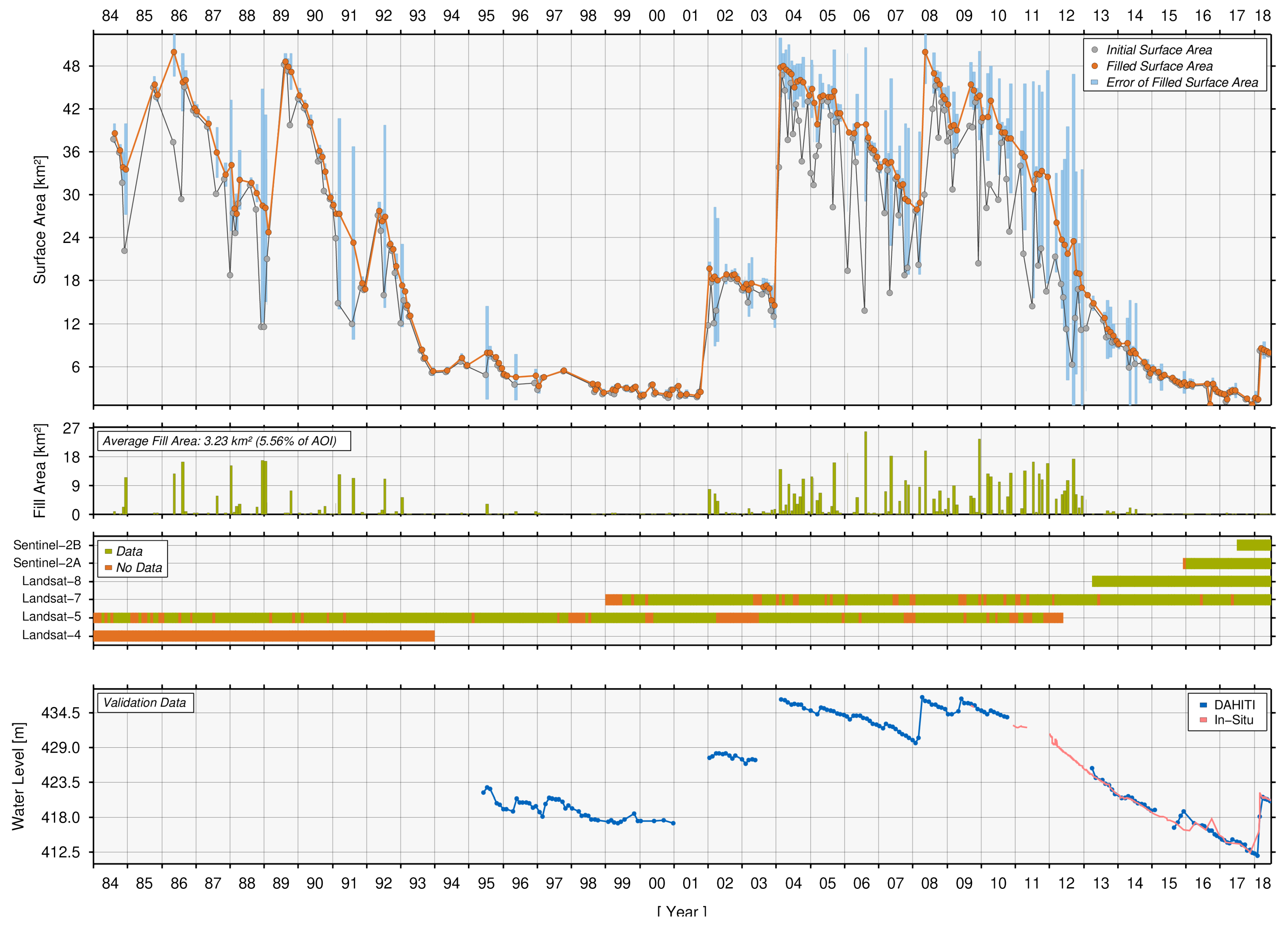
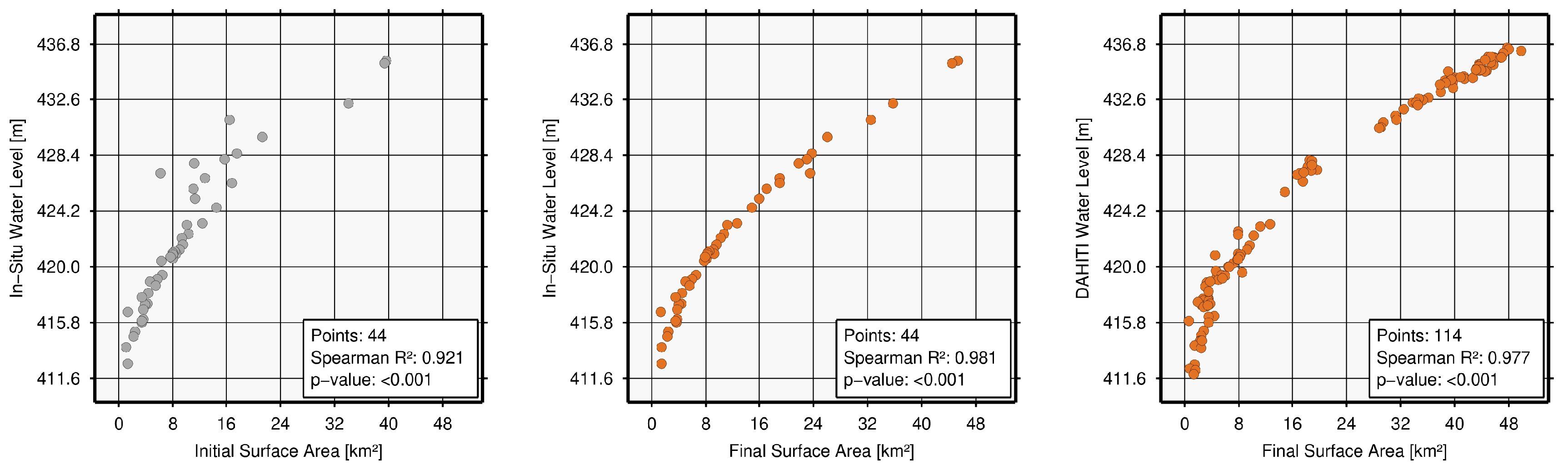
4.2.2. Poço da Cruz, Reservoir
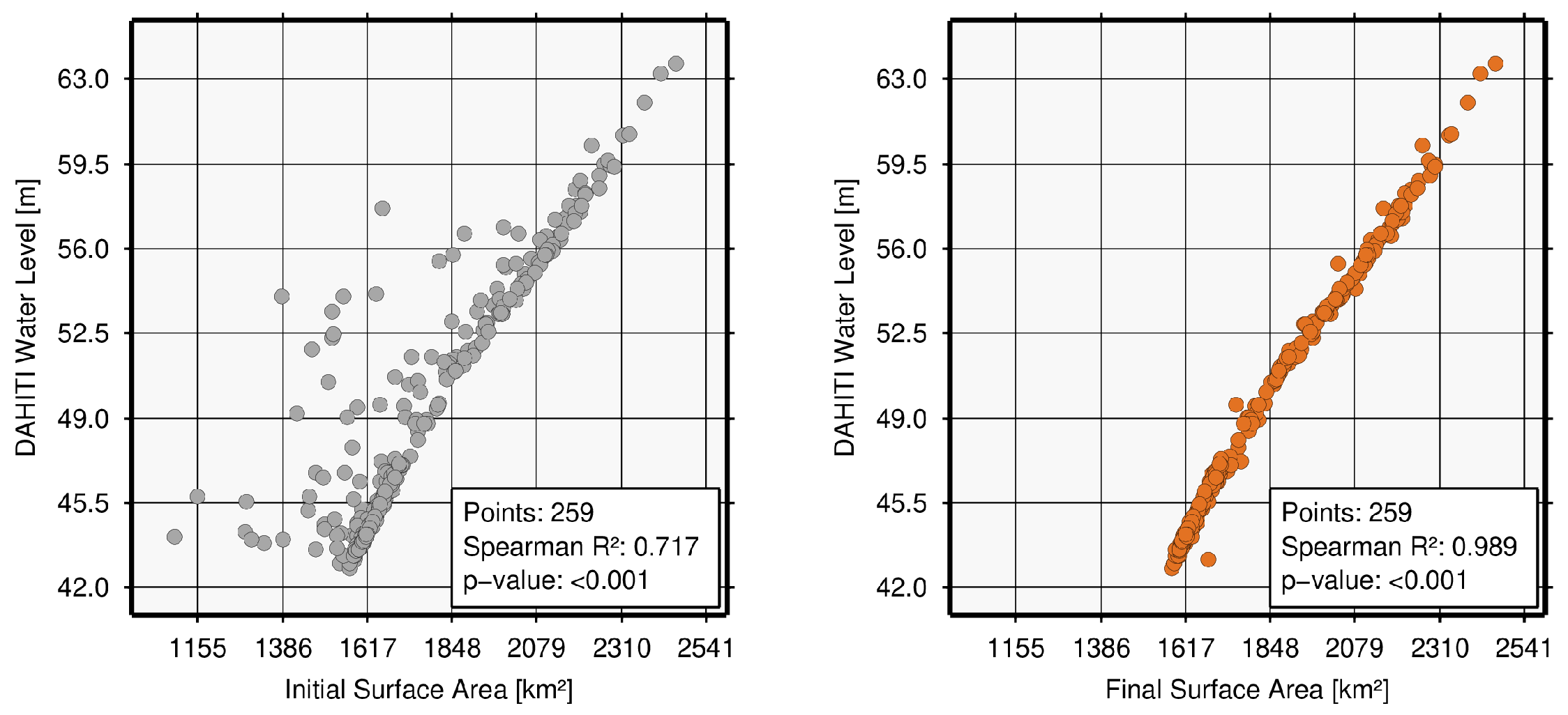
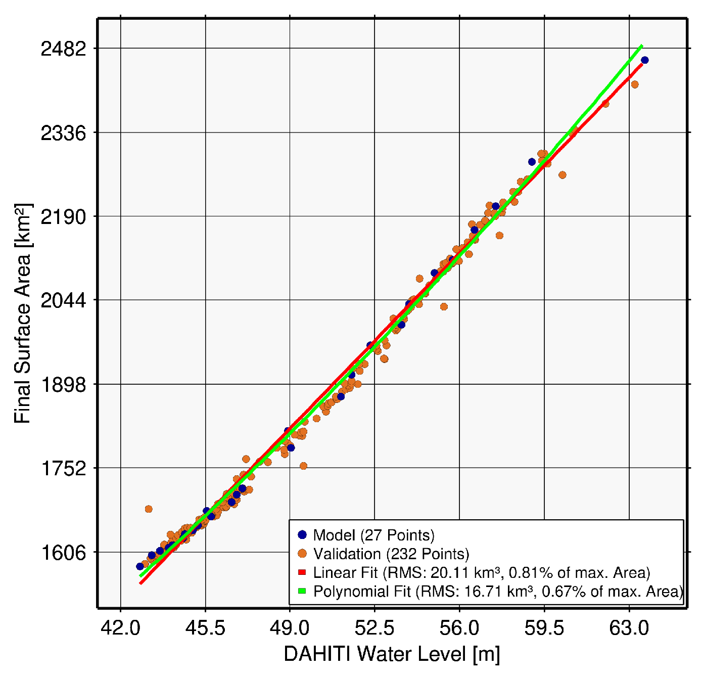
4.2.3. Tharthar, Lake
4.3. Quality Assessment and Discussion
5. Conclusions
6. Data Availability
Supplementary Materials
Author Contributions
Funding
Acknowledgments
Conflicts of Interest
References
- Shiklomanov, I. World Fresh Water Resources. In Water in Crisis—A Guide to the World’s Fresh Water Resources; Gleick, P., Ed.; Oxford University Press: Oxford, UK, 1993; Chapter 2; pp. 13–23. [Google Scholar]
- Guha-Sapir, D.; Vos, F. Quantifying Global Environmental Change Impacts: Methods, Criteria and Definitions for Compiling Data on Hydro-meteorological Disasters. In Coping with Global Environmental Change, Disasters and Security: Threats, Challenges, Vulnerabilities and Risks; Brauch, H.G., Oswald Spring, U., Mesjasz, C., Grin, J., Kameri-Mbote, P., Chourou, B., Dunay, P., Birkmann, J., Eds.; Springer: Berlin/Heidelberg, Germany, 2011; pp. 693–717. [Google Scholar] [CrossRef]
- Hasan, M.; Moody, A.; Benninger, L.; Hedlund, H. How war, drought, and dam management impact water supply in the Tigris and Euphrates Rivers. Ambio 2018. [Google Scholar] [CrossRef] [PubMed]
- Global Runoff Data Center: Statistics Based on GRDC Station Catalogue from 2018-10-19. Available online: https://www.bafg.de/SharedDocs/ExterneLinks/GRDC/grdc_stations_ftp.html?nn=201352 (accessed on 25 January 2019).
- Memon, A.A.; Muhammad, S.; Rahman, S.; Haq, M. Flood monitoring and damage assessment using water indices: A case study of Pakistan flood-2012. Egypt. J. Remote Sens. Space Sci. 2015, 18, 99–106. [Google Scholar] [CrossRef]
- Amani, M.; Salehi, B.; Mahdavi, S.; Brisco, B. Spectral analysis of wetlands using multi-source optical satellite imagery. ISPRS J. Photogramm. Remote Sens. 2018, 144, 119–136. [Google Scholar] [CrossRef]
- DeVries, B.; Huang, C.; Lang, M.W.; Jones, J.W.; Huang, W.; Creed, I.F.; Carroll, M.L. Automated Quantification of Surface Water Inundation in Wetlands Using Optical Satellite Imagery. Remote Sens. 2017, 9, 807. [Google Scholar] [CrossRef]
- Singh, A.; Seitz, F.; Schwatke, C. Inter-annual water storage changes in the Aral Sea from multi-mission satellite altimetry, optical remote sensing, and GRACE satellite gravimetry. Remote Sens. Environ. 2012, 123, 187–195. [Google Scholar] [CrossRef]
- Ghanavati, E.; Firouzabadi, P.Z.; Jangi, A.A.; Khosravi, S. Monitoring geomorphologic changes using Landsat TM and ETM+ data in the Hendijan River delta, southwest Iran. Int. J. Remote Sens. 2008, 29, 945–959. [Google Scholar] [CrossRef]
- Xu, H. Modification of normalised difference water index (NDWI) to enhance open water features in remotely sensed imagery. Int. J. Remote Sens. 2006, 27, 3025–3033. [Google Scholar] [CrossRef]
- Ding, F. Study on Information Extraction of Water Body with a New Water Index (NWI). Sci. Surv. Mapp. 2009, 34, 155–157. [Google Scholar]
- Feyisa, G.L.; Meilby, H.; Fensholt, R.; Proud, S.R. Automated Water Extraction Index: A new technique for surface water mapping using Landsat imagery. Remote Sens. Environ. 2014, 140, 23–35. [Google Scholar] [CrossRef]
- Kauth, R.; Thomas, G. TheTasseled Cap—A graphic description of thespectral-temporal development of agricul-tural crops as seen by Landsat. In Proceedings of the Symposium on Machine Processing of Remotely Sensed Data, West Lafayette, IN, USA, 29 June–1 July 1976; Volume 4B, pp. 41–51. [Google Scholar]
- Gomez, C.; White, J.C.; Wulder, M.A. Optical remotely sensed time series data for land cover classification: A review. ISPRS J. Photogramm. Remote Sens. 2016, 116, 55–72. [Google Scholar] [CrossRef]
- Otsu, N. A Threshold Selection Method from Gray-Level Histograms. IEEE Trans. Syst. Man Cybern. 1979, 9, 62–66. [Google Scholar] [CrossRef]
- Feng, M.; Sexton, J.O.; Channan, S.; Townshend, J.R. A global, high-resolution (30-m) inland water body dataset for 2000: First results of a topographic-spectral classification algorithm. Int. J. Digit. Earth 2016, 9, 113–133. [Google Scholar] [CrossRef]
- Pekel, J.F.; Cottam, A.; Gorelick, N.; Belward, A.S. High-resolution mapping of global surface water and its long-term changes. Nature 2016, 540, 418–422. [Google Scholar] [CrossRef]
- Klein, I.; Gessner, U.; Dietz, A.J.; Kuenzer, C. Global WaterPack—A 250m resolution dataset revealing the daily dynamics of global inland water bodies. Remote Sens. Environ. 2017, 198, 345–362. [Google Scholar] [CrossRef]
- Markert, K.N.; Chishtie, F.; Anderson, E.R.; Saah, D.; Griffin, R.E. On the merging of optical and SAR satellite imagery for surface water mapping applications. Results Phys. 2018, 9, 275–277. [Google Scholar] [CrossRef]
- Zhang, S.; Gao, H.; Naz, B.S. Monitoring reservoir storage in South Asia from multisatellite remote sensing. Water Resour. Res. 2014, 50, 8927–8943. [Google Scholar] [CrossRef]
- Busker, T.; de Roo, A.; Gelati, E.; Schwatke, C.; Adamovic, M.; Bisselink, B.; Pekel, J.F.; Cottam, A. A global lake and reservoir volume analysis using a surface water dataset and satellite altimetry. Hydrol. Earth Syst. Sci. 2019, 23, 669–690. [Google Scholar] [CrossRef]
- Irons, J.R.; Dwyer, J.L.; Barsi, J.A. The next Landsat satellite: The Landsat Data Continuity Mission. Remote Sens. Environ. 2012, 122, 11–21. [Google Scholar] [CrossRef]
- Gorelick, N.; Hancher, M.; Dixon, M.; Ilyushchenko, S.; Thau, D.; Moore, R. Google Earth Engine: Planetary-scale geospatial analysis for everyone. Remote Sens. Environ. 2017, 202, 18–27. [Google Scholar] [CrossRef]
- Foga, S.; Scaramuzza, P.L.; Guo, S.; Zhu, Z.; Dilley, R.D.; Beckmann, T.; Schmidt, G.L.; Dwyer, J.L.; Hughes, M.J.; Laue, B. Cloud detection algorithm comparison and validation for operational Landsat data products. Remote Sens. Environ. 2017, 194, 379–390. [Google Scholar] [CrossRef]
- ESA. SENTINEL-2 ESA’s Optical High-Resolution Mission for GMES Operational Services, SP-1322/2; Technical Report; ESA: Paris, France, 2012. [Google Scholar]
- ESA. Sen2Cor—Configuration and User Manual, S2-PDGS-MPC-L2A-SUM-V2.5.5; Technical Report; ESA: Paris, France, 2018. [Google Scholar]
- Zhu, Z.; Wang, S.; Woodcock, C.E. Improvement and expansion of the Fmask algorithm: Cloud, cloud shadow, and snow detection for Landsats 4-7, 8, and Sentinel 2 images. Remote Sens. Environ. 2015, 159, 269–277. [Google Scholar] [CrossRef]
- Da Silva, J.S.; Calmant, S.; Seyler, F.; Filho, O.C.R.; Cochonneau, G.; Mansur, W.J. Water levels in the Amazon basin derived from the ERS 2 and ENVISAT radar altimetry missions. Remote Sens. Environ. 2010, 114, 2160–2181. [Google Scholar] [CrossRef]
- Dettmering, D.; Schwatke, C.; Boergens, E.; Seitz, F. Potential of ENVISAT Radar Altimetry for Water Level Monitoring in the Pantanal Wetland. Remote Sens. 2016, 8, 596. [Google Scholar] [CrossRef]
- Crétaux, J.F.; Jelinski, W.; Calmant, S.; Kouraev, A.; Vuglinski, V.; Bergé-Nguyen, M.; Gennero, M.C.; Nino, F.; Rio, R.A.D.; Cazenave, A.; et al. SOLS: A lake database to monitor in the Near Real Time water level and storage variations from remote sensing data. Adv. Space Res. 2011, 47, 1497–1507. [Google Scholar] [CrossRef]
- Schwatke, C.; Dettmering, D.; Bosch, W.; Seitz, F. DAHITI—An innovative approach for estimating water level time series over inland waters using multi-mission satellite altimetry. Hydrol. Earth Syst. Sci. 2015, 19, 4345–4364. [Google Scholar] [CrossRef]
- McFeeters, S.K. The use of the Normalized Difference Water Index (NDWI) in the delineation of open water features. Int. J. Remote Sens. 1996, 17, 1425–1432. [Google Scholar] [CrossRef]
- Haibo, Y.; Zongmin, W.; Hongling, Z.; Yu, G. Water Body Extraction Methods Study Based on RS and GIS. Procedia Environ. Sci. 2011, 10 Pt C, 2619–2624. [Google Scholar] [CrossRef]
- Crist, E. A TM Tasseled Cap Equivalent Transformation for Reflectance Factor Data. Remote Sens. Environ. 1985, 17, 301–306. [Google Scholar] [CrossRef]
- Rosenfeld, A.; Pfaltz, J.L. Sequential Operations in Digital Picture Processing. J. ACM 1966, 13, 471–494. [Google Scholar] [CrossRef]
- Beck, H.E.; Zimmermann, N.E.; McVicar, T.R.; Vergopolan, N.; Berg, A.; Wood, E.F. Present and future Köppen-Geiger climate classification maps at 1-km resolution. Sci. Data 2018, 5. [Google Scholar] [CrossRef]
- Fick, S.E.; Hijmans, R.J. WorldClim 2: New 1-km spatial resolution climate surfaces for global land areas. Int. J. Climatol. 2017, 37, 4302–4315. [Google Scholar] [CrossRef]
- Wilson, A.M.; Jetz, W. Remotely Sensed High-Resolution Global Cloud Dynamics for Predicting Ecosystem and Biodiversity Distributions. PLoS Biol. 2016, 14, 1–20. [Google Scholar] [CrossRef] [PubMed]
- Wulder, M.A.; White, J.C.; Loveland, T.R.; Woodcock, C.E.; Belward, A.S.; Cohen, W.B.; Fosnight, E.A.; Shaw, J.; Masek, J.G.; Roy, D.P. The global Landsat archive: Status, consolidation, and direction. Remote Sens. Environ. 2016, 185, 271–283. [Google Scholar] [CrossRef]


| Band Description | Landsat-4,-5,-7 (TM and ETM+) | Landsat-8 (OLI) | Sentinel-2A,-2B | Standard Name |
|---|---|---|---|---|
| Blue | Band 1 | Band 2 | Band 2 | |
| Green | Band 2 | Band 3 | Band 3 | |
| Red | Band 3 | Band 4 | Band 4 | |
| Near-Infrared (NIR) | Band 4 | Band 5 | Band 8 | |
| Short Wave Infrared 1 (SWIR1) | Band 5 | Band 6 | Band 11 | |
| Short Wave Infrared 2 (SWIR2) | Band 7 | Band 7 | Band 12 | |
| Mask (Clouds, Shadow, etc.) | CFmask | CFmask | Fmask4.0 |
| Lake/Reservoir | Station Name | Station ID | Source |
|---|---|---|---|
| Claiborne | Aycock | 07364840 | USGS |
| Clear | Clarence | 07352895 | USGS |
| Cooper | Cooper | 07342495 | USGS |
| Forggen | Rosshaupten | 12001301 | BEA |
| Lewisville | Lewisville | 08052800 | USGS |
| Mead | n.a. | n.a. | USGS |
| Murray | Columbia | 02168500 | USGS |
| Nova Ponte | n.a. | n.a. | ANA |
| Poço da Cruz | n.a. | n.a. | ANA |
| Ray Roberts | Pilot Point, TX | 08051100 | USGS |
| Richland Chambers | Kerens, TX | 08064550 | USGS |
| Salton Sea | Westmorland | 10254005 | USGS |
| Sam Rayburn | Jasper | 08039300 | USGS |
| Tawakoni | Wills Point | 08017400 | USGS |
| Toledo Bend | Burkeville | 08025350 | USGS |
| Input Value (based on 5 Water Indexes) | Monthly Land-Water Mask | Index Error |
|---|---|---|
| 5 Water pixels | Water (1) | No |
| 4 Water pixels | Water (1) | Yes |
| 3 Water pixels | Data gap | No |
| 2 Water pixels | Data gap | No |
| 1 Water pixel | Land (0) | Yes |
| 0 Water pixels | Land (0) | No |
| Data gap | Data gap | No |
| Target Name, Country (DAHITI ID) | Max. Water Level Var. [m] | Max. Surface Area [km] | Max. Shore Length [km] | Ratio Area/Shore | Climate Zone [36] | Annual Rainfall [37] [mm/y] | Annual Clouds [38] [%] |
|---|---|---|---|---|---|---|---|
| Aragon, Spain (10297) | 33.45 | 22.14 | 93.53 | 0.24 | Cfb | 738 | 52 |
| Bankim, Cameroon (3560) | 14.17 | 336.56 | 2154.36 | 0.16 | Aw | 1749 | 53 |
| Boston, China (226) | 4.36 | 1226.56 | 1558.10 | 0.79 | BWk | 79 | 47 |
| Claiborne, USA (10472) | 4.30 | 25.54 | 138.31 | 0.18 | Cfa | 1340 | 53 |
| Clear, USA (10496) | 2.26 | 49.94 | 267.63 | 0.19 | Cfa | 1375 | 52 |
| Cooper, USA (10505) | 8.07 | 82.68 | 186.64 | 0.44 | Cfa | 1122 | 49 |
| Dagze, China (10425) | 8.12 | 326.71 | 234.66 | 1.39 | BSk | 260 | 47 |
| Enriquillo, Dom. Rep. (11521) | 10.12 | 354.14 | 190.65 | 1.86 | BSh | 566 | 35 |
| Eucumbene, Australia (64) | 37.57 | 140.98 | 458.60 | 0.31 | Cfb | 799 | 50 |
| Fairfield, USA (2672) | 3.05 | 9.84 | 60.23 | 0.16 | Cfa | 1021 | 50 |
| Forggen, Germany (10341) | 9.86 | 16.73 | 47.97 | 0.35 | Dfb | 1320 | 65 |
| Jacarei, Brazil (10345) | 28.22 | 49.39 | 323.28 | 0.15 | Cfb | 1453 | 56 |
| Jenipapeiro, Brazil (3581) | 15.76 | 11.05 | 101.89 | 0.11 | Aw | 914 | 59 |
| Lagdo, Cameroon (1472) | 9.33 | 759.42 | 1327.21 | 0.57 | Aw | 1006 | 51 |
| Lewisville, USA (11327) | 4.38 | 130.33 | 533.76 | 0.24 | Cfa | 938 | 44 |
| Massingir, Mozambique (606) | 20.81 | 189.09 | 249.58 | 0.76 | BSh | 472 | 42 |
| Mead, USA (204) | 43.56 | 598.29 | 1350.23 | 0.44 | BWh | 133 | 24 |
| Murray, USA (8852) | 3.92 | 196.46 | 1038.15 | 0.19 | Cfa | 1181 | 50 |
| Nova Ponte, Brazil (10351) | 32.98 | 400.05 | 1936.99 | 0.21 | Aw | 1540 | 51 |
| Orellana, Spain (11415) | 6.41 | 52.76 | 282.09 | 0.19 | Csa | 535 | 40 |
| Pau dos Ferros, Brazil (8692) | 13.90 | 11.58 | 67.27 | 0.17 | Aw | 853 | 56 |
| Pires Ferreira, Brazil (8671) | 19.91 | 85.05 | 509.66 | 0.17 | Aw | 974 | 57 |
| Poço da Cruz, Brazil (8702) | 24.62 | 58.07 | 382.99 | 0.15 | BSh | 552 | 65 |
| Ray Roberts, USA (10146) | 5.74 | 132.16 | 487.12 | 0.27 | Cfa | 990 | 45 |
| Richland Chambers, USA (8814) | 3.70 | 182.87 | 410.50 | 0.45 | Cfa | 1004 | 49 |
| Salton Sea, USA (71) | 2.78 | 989.59 | 417.88 | 2.37 | BWh | 71 | 22 |
| Sam Rayburn, USA (10246) | 5.97 | 448.34 | 1204.62 | 0.37 | Cfa | 1260 | 50 |
| Tawakoni, USA (8813) | 3.70 | 160.85 | 405.58 | 0.40 | Cfa | 1074 | 44 |
| Tharthar, Iraq (122) | 21.07 | 2491.37 | 1183.21 | 2.11 | BWh | 130 | 27 |
| Toledo Bend, USA (10247) | 4.20 | 659.44 | 1733.77 | 0.38 | Cfa | 1289 | 49 |
| Tundes Grandes, Argentina (4475) | 3.05 | 331.27 | 809.82 | 0.41 | Cfa | 840 | 45 |
| Zujar, Spain (10301) | 20.26 | 153.56 | 730.30 | 0.21 | BSk | 517 | 40 |
| Target Name, Country (ID) | Data Availability | Monthly | Validation Gauge | Validation Altimetry | Area Error w.r.t AOI | ||||||||||||
|---|---|---|---|---|---|---|---|---|---|---|---|---|---|---|---|---|---|
| L4 [%] | L5 [%] | L7 [%] | L8 [%] | S2A [%] | S2B [#] | Masks [#] | Points [#] | Initial | Final | Impr. | Points [#] | Initial | Final | Impr. | km | [%] | |
| Aragon, Spain (10297) | 3.3 | 90.6 | 88.9 | 100.0 | 100.0 | 100.0 | 310 | no data | 125 | 0.698 | 0.823 | 0.125 | 1.21 | 6.08 | |||
| Bankim, Cameroon (3560) | 4.2 | 5.3 | 81.2 | 100.0 | 100.0 | 100.0 | 114 | no data | 80 | 0.464 | 0.922 | 0.458 | 30.50 | 9.68 | |||
| Boston, China (226) | 5.0 | 80.1 | 94.9 | 100.0 | 100.0 | 100.0 | 208 | no data | 115 | 0.402 | 0.896 | 0.494 | 38.95 | 3.37 | |||
| Claiborne, USA (10472) | 0.8 | 90.9 | 95.7 | 100.0 | 96.8 | 100.0 | 298 | 212 | 0.071 | 0.267 | 0.196 1 | no data | 0.66 | 2.93 | |||
| Clear, USA (10496) | 0.8 | 84.5 | 96.6 | 96.8 | 96.8 | 100.0 | 214 | 151 | 0.199 | 0.343 | 0.144 1 | no data | 2.52 | 6.31 | |||
| Cooper, USA (10505) | 0.8 | 87.1 | 96.2 | 100.0 | 96.8 | 100.0 | 259 | 172 | 0.779 | 0.940 | 0.161 1 | no data | 1.84 | 2.36 | |||
| Dagze, China (10425) | 2.5 | 59.8 | 90.6 | 100.0 | 96.8 | 100.0 | 151 | no data | 67 | 0.462 | 0.900 | 0.438 | 8.98 | 2.78 | |||
| Enriquillo, Dom. Rep. (11521) | 7.5 | 24.0 | 67.1 | 100.0 | 96.8 | 100.0 | 196 | no data | 95 | 0.641 | 0.949 | 0.308 | 14.26 | 4.09 | |||
| Eucumbene, Australia (64) | 0.0 | 68.9 | 96.6 | 98.4 | 100.0 | 100.0 | 289 | no data | 95 | 0.936 | 0.966 | 0.030 | 4.84 | 3.53 | |||
| Fairfield, USA (2672) | 0.8 | 78.6 | 84.6 | 87.3 | 96.8 | 100.0 | 307 | no data | 96 | 0.212 | 0.440 | 0.228 | 0.30 | 3.45 | |||
| Forggen, Germany (10341) | 10.8 | 79.5 | 82.5 | 100.0 | 100.0 | 100.0 | 183 | 179 | 0.595 | 0.770 | 0.175 2 | no data | 0.77 | 5.11 | |||
| Jacarei, Brazil (10345) | 0.8 | 69.8 | 83.3 | 98.4 | 100.0 | 100.0 | 282 | no data | 65 | 0.847 | 0.970 | 0.123 | 1.87 | 4.01 | |||
| Jenipapeiro, Brazil (3581) | 0.0 | 80.1 | 84.6 | 100.0 | 96.8 | 100.0 | 219 | no data | 82 | 0.751 | 0.967 | 0.216 | 0.68 | 7.47 | |||
| Lagdo, Cameroon (1472) | 5.8 | 6.2 | 83.3 | 98.4 | 100.0 | 100.0 | 161 | no data | 101 | 0.062 | 0.796 | 0.734 | 56.89 | 7.63 | |||
| Lewisville, USA (11327) | 0.8 | 83.9 | 88.5 | 96.8 | 96.8 | 100.0 | 291 | 265 | 0.736 | 0.949 | 0.213 1 | 36 | 0.410 | 0.672 | 0.262 | 2.93 | 2.43 |
| Massingir, Mozambique (606) | 6.7 | 41.9 | 79.1 | 96.8 | 100.0 | 100.0 | 240 | no data | 64 | 0.589 | 0.957 | 0.368 | 6.72 | 4.99 | |||
| Mead, USA (204) | 7.5 | 91.5 | 97.0 | 100.0 | 100.0 | 100.0 | 347 | 145 | 0.949 | 0.984 | 0.035 1 | 151 | 0.979 | 0.993 | 0.014 | 11.56 | 1.95 |
| Murray, USA (8852) | 0.8 | 92.4 | 94.0 | 95.2 | 96.8 | 100.0 | 302 | 297 | 0.601 | 0.863 | 0.262 1 | 73 | 0.647 | 0.710 | 0.063 | 4.91 | 2.69 |
| Nova Ponte, Brazil (10351) | 0.8 | 82.1 | 94.4 | 100.0 | 96.8 | 100.0 | 189 | 189 | 0.956 | 0.993 | 0.037 3 | 88 | 0.912 | 0.983 | 0.071 | 11.52 | 2.75 |
| Orellana, Spain (11415) | 2.5 | 85.9 | 85.0 | 100.0 | 100.0 | 100.0 | 330 | no data | 57 | 0.293 | 0.836 | 0.543 | 2.07 | 4.23 | |||
| Pau dos Ferros, Brazil (8692) | 0.0 | 69.2 | 70.9 | 98.4 | 100.0 | 100.0 | 201 | no data | 59 | 0.907 | 0.971 | 0.064 | 0.60 | 5.59 | |||
| Pires Ferreira, Brazil (8671) | 1.7 | 62.8 | 70.9 | 100.0 | 100.0 | 100.0 | 141 | no data | 67 | 0.772 | 0.913 | 0.141 | 6.36 | 8.03 | |||
| Poço da Cruz, Brazil (8702) | 0.0 | 79.5 | 85.0 | 100.0 | 96.8 | 100.0 | 228 | 44 | 0.921 | 0.981 | 0.060 3 | 114 | 0.912 | 0.977 | 0.065 | 3.23 | 5.56 |
| Ray Roberts, USA (10146) | 0.8 | 83.6 | 88.5 | 98.4 | 96.8 | 100.0 | 290 | 273 | 0.777 | 0.934 | 0.157 1 | 106 | 0.591 | 0.910 | 0.319 | 2.18 | 1.59 |
| Richland Chambers, USA (8814) | 2.5 | 91.2 | 96.6 | 98.4 | 96.8 | 100.0 | 289 | 221 | 0.442 | 0.883 | 0.441 1 | 122 | 0.419 | 0.879 | 0.460 | 2.31 | 1.31 |
| Salton Sea, USA (71) | 8.3 | 91.8 | 97.0 | 100.0 | 100.0 | 100.0 | 352 | 326 | 0.536 | 0.911 | 0.375 1 | 127 | 0.565 | 0.954 | 0.389 | 8.62 | 0.89 |
| Sam Rayburn, USA (10246) | 1.7 | 93.0 | 96.2 | 100.0 | 96.8 | 100.0 | 283 | 246 | 0.472 | 0.907 | 0.435 1 | 94 | 0.489 | 0.779 | 0.290 | 11.97 | 2.77 |
| Tawakoni, USA (8813) | 1.7 | 93.0 | 96.6 | 100.0 | 96.8 | 100.0 | 292 | 207 | 0.580 | 0.912 | 0.332 1 | 89 | 0.505 | 0.903 | 0.398 | 2.10 | 1.38 |
| Tharthar, Iraq (122) | 21.7 | 86.5 | 91.0 | 100.0 | 100.0 | 100.0 | 327 | no data | 259 | 0.717 | 0.989 | 0.272 | 67.80 | 2.72 | |||
| Toledo Bend, USA (10247) | 1.7 | 93.0 | 96.2 | 100.0 | 96.8 | 100.0 | 257 | 137 | 0.522 | 0.876 | 0.354 1 | 89 | 0.428 | 0.802 | 0.374 | 14.80 | 2.32 |
| Tundes Grandes, Argentina (4475) | 15.0 | 71.3 | 94.4 | 100.0 | 93.5 | 83.3 | 206 | no data | 105 | 0.866 | 0.940 | 0.074 | 13.00 | 4.34 | |||
| Zujar, Spain (10301) | 2.5 | 85.9 | 85.0 | 100.0 | 100.0 | 100.0 | 350 | no data | 87 | 0.630 | 0.838 | 0.208 | 4.92 | 3.38 | |||
| Target Name, Country (ID) | Hypsometry (Linear) | Hypsometry (2nd Deg.) | ||||
|---|---|---|---|---|---|---|
| Model Points [#] | Validation Points [#] | RMS [km] | wrt. Area [%] | RMS [km] | wrt. Area [%] | |
| Aragon, Spain (10297) | 14 | 111 | 1.14 | 5.16 | 1.14 | 5.16 |
| Bankim, Cameroon (3560) | 9 | 71 | 21.30 | 6.33 | 19.26 | 5.72 |
| Boston, China (226) | 13 | 102 | 18.70 | 1.52 | 18.20 | 1.48 |
| Claiborne, USA (10472) | 23 | 189 | 0.65 | 2.53 | 1.07 | 4.20 |
| Clear, USA (10496) | 16 | 135 | 3.92 | 7.85 | 3.74 | 7.48 |
| Cooper, USA (10505) | 19 | 153 | 2.03 | 2.48 | 1.94 | 2.35 |
| Dagze, China (10425) | 7 | 60 | 3.54 | 1.08 | 3.68 | 1.13 |
| Enriquillo, Dom. Rep. (11521) | 11 | 84 | 13.97 | 3.94 | 11.59 | 3.27 |
| Eucumbene, Australia (64) | 11 | 84 | 2.58 | 1.83 | 2.67 | 1.90 |
| Fairfield, USA (2672) | 11 | 85 | 0.28 | 2.85 | 0.28 | 2.88 |
| Forggen, Germany (10341) | 19 | 160 | 0.83 | 4.94 | 0.84 | 5.02 |
| Jacarei, Brazil (10345) | 8 | 57 | 1.56 | 3.17 | 1.75 | 3.55 |
| Jenipapeiro, Brazil (3581) | 10 | 72 | 0.26 | 2.33 | 0.26 | 2.33 |
| Lagdo, Cameroon (1472) | 11 | 90 | 39.19 | 5.16 | 40.07 | 5.28 |
| Lewisville, USA (11327) | 28 | 237 | 2.85 | 2.19 | 2.42 | 1.86 |
| Massingir, Mozambique (606) | 8 | 56 | 6.30 | 3.33 | 4.03 | 2.13 |
| Mead, USA (204) | 16 | 129 | 5.21 | 0.87 | 3.97 | 0.66 |
| Murray, USA (8852) | 31 | 266 | 2.64 | 1.34 | 2.34 | 1.19 |
| Nova Ponte, Brazil (10351) | 20 | 169 | 6.07 | 1.52 | 5.47 | 1.37 |
| Orellana, Spain (11415) | 7 | 50 | 1.26 | 2.39 | 1.26 | 2.38 |
| Pau dos Ferros, Brazil (8692) | 7 | 52 | 0.80 | 6.89 | 0.51 | 4.40 |
| Pires Ferreira, Brazil (8671) | 7 | 60 | 5.45 | 6.41 | 6.80 | 7.99 |
| Poço da Cruz, Brazil (8702) | 5 | 39 | 3.53 | 6.07 | 1.10 | 1.90 |
| Ray Roberts, USA (10146) | 30 | 255 | 2.88 | 2.18 | 2.74 | 2.07 |
| Richland Chambers, USA (8814) | 23 | 198 | 2.34 | 1.28 | 2.19 | 1.20 |
| Salton Sea, USA (71) | 34 | 292 | 4.58 | 0.46 | 4.52 | 0.46 |
| Sam Rayburn, USA (10246) | 26 | 220 | 10.07 | 2.25 | 5.96 | 1.33 |
| Tawakoni, USA (8813) | 22 | 185 | 2.74 | 1.70 | 2.36 | 1.47 |
| Tharthar, Iraq (122) | 27 | 232 | 20.11 | 1.59 | 16.71 | 1.21 |
| Toledo Bend, USA (10247) | 15 | 122 | 10.48 | 0.81 | 7.96 | 0.67 |
| Tundes Grandes, Argentina (4475) | 12 | 93 | 8.43 | 2.55 | 8.11 | 2.45 |
| Zujar, Spain (10301) | 10 | 77 | 5.75 | 3.74 | 5.75 | 3.75 |
© 2019 by the authors. Licensee MDPI, Basel, Switzerland. This article is an open access article distributed under the terms and conditions of the Creative Commons Attribution (CC BY) license (http://creativecommons.org/licenses/by/4.0/).
Share and Cite
Schwatke, C.; Scherer, D.; Dettmering, D. Automated Extraction of Consistent Time-Variable Water Surfaces of Lakes and Reservoirs Based on Landsat and Sentinel-2. Remote Sens. 2019, 11, 1010. https://doi.org/10.3390/rs11091010
Schwatke C, Scherer D, Dettmering D. Automated Extraction of Consistent Time-Variable Water Surfaces of Lakes and Reservoirs Based on Landsat and Sentinel-2. Remote Sensing. 2019; 11(9):1010. https://doi.org/10.3390/rs11091010
Chicago/Turabian StyleSchwatke, Christian, Daniel Scherer, and Denise Dettmering. 2019. "Automated Extraction of Consistent Time-Variable Water Surfaces of Lakes and Reservoirs Based on Landsat and Sentinel-2" Remote Sensing 11, no. 9: 1010. https://doi.org/10.3390/rs11091010
APA StyleSchwatke, C., Scherer, D., & Dettmering, D. (2019). Automated Extraction of Consistent Time-Variable Water Surfaces of Lakes and Reservoirs Based on Landsat and Sentinel-2. Remote Sensing, 11(9), 1010. https://doi.org/10.3390/rs11091010