Global White-Sky and Black-Sky FAPAR Retrieval Using the Energy Balance Residual Method: Algorithm and Validation

Abstract

The fraction of absorbed photosynthetically active radiation by vegetation (FAPAR) is a key variable in describing the light absorption ability of the vegetation canopy. Most global FAPAR products, such as MCD15A2H and GEOV1, correspond to FAPAR under black-sky conditions at the satellite overpass time only. In this paper, we aim to produce both the global white-sky and black-sky FAPAR products based on the moderate resolution imaging spectroradiometer (MODIS) visible (VIS) albedo, leaf area index (LAI), and clumping index (CI) products. Firstly, a non-linear spectral mixture model (NSM) was designed to retrieve the soil visible (VIS) albedo. The global soil VIS albedo and its dynamics were successfully mapped at a resolution of 500 m using the MCD43A3 VIS albedo product and the MCD15A2H LAI product. Secondly, a method based on the energy balance residual (EBR) principle was presented to retrieve the white-sky and black-sky FAPAR using the MODIS broadband VIS albedo (white-sky and black-sky) product (MCD43A3), the LAI product (MCD15A2H) and CI products. Finally, the two EBR FAPAR products were compared with the MCD15A2H and Geoland2/BioPar version 1 (GEOV1) black-sky FAPAR products. A comparison of the results indicates that these FAPAR products show similar spatial and seasonal patterns. Direct validation using FAPAR observations from the Validation of Land European Remote sensing Instrument (VALERI) project demonstrates that the EBR black-sky FAPAR product was more accurate and had a lower bias (R² = 0.917, RMSE = 0.088, and bias = −2.8 %) than MCD15A2H (R² = 0.901, RMSE = 0.096, and bias = 7.6 % ) and GEOV1 (R² = 0.868, RMSE = 0.105, and bias = 6.1%).

1. Introduction

The fraction of absorbed photosynthetically active radiation (FAPAR) is defined as the fraction of intercepted photosynthetically active radiation (PAR) which is absorbed by the canopy. The FAPAR is a key variable in describing the exchange of fluxes of energy, mass, and momentum between the surface and atmosphere in global models of climate, hydrology, biogeochemistry, agriculture, and ecology [1,2]. With the significant increase in global remotely-sensed biophysical datasets, FAPAR is identified as one of the key terrestrial products [2,3,4].

The radiative transfer process within the canopy is different for diffuse and direct PARs. In general, the diffuse PAR has more probability to arrive at the bottom of the canopy than the direct PAR. The probability of the direct PAR intercepted by the canopy usually increases with the increase of the solar zenith angle (SZA) [5,6]. Numerous diurnal observations and theoretical simulations have also shown that FAPAR is larger under overcast-sky (white-sky) than under clear-sky (or blue-sky) conditions. For the diurnal pattern, FAPAR is usually found to be smaller at noon with smaller SZA [7,8,9,10], especially for regions covered with sparse vegetation [5,11,12,13]. The FAPAR of direct radiation and diffuse radiation are defined as “black-sky FAPAR” and “white-sky FAPAR”, respectively. To estimate the instantaneous total FAPAR or daily integrated FAPAR under natural conditions, both white-sky and black-sky FAPARs are needed.

There are several available global FAPAR datasets, including the MISR (multi-angle imaging spectroradiometer) [14], MODIS (moderate resolution imaging spectroradiometer) [3,15], MERIS (medium resolution imaging spectrometer) [16,17], SeaWiFS (sea-viewing wide field-of-view sensor) [18], GLOBCARBON [19], CYCLOPES [20], Geoland2/BioPar version 1 (GEOV1) [6], and GLASS (global land surface satellite) [21] products. These global FAPAR products have been widely validated, with reported errors varying from 0.08 to 0.23 [21,22,23,24,25,26,27]. However, most of the global products are black-sky FAPAR (direct radiation only) or FAPAR under instantaneous illumination condition at the satellite overpass time [6,13,21]. Previous studies have proved that total FAPAR would be underestimated without considering the white-sky FAPAR, and the current models also underestimated total FAPAR because of the simplification of radiative transfer processes [8,13]. Therefore, it is important to develop algorithms for new white-sky and black-sky FAPAR.

Algorithms for estimation of FAPAR from satellite remote sensing data can be divided into two groups: empirical methods and physical methods [6,14,15,18,20]. The empirical methods use the statistical relationships between FAPAR and vegetation indices to estimate FAPAR. [3,5,11,14,28,29,30]. However, these statistical relationships are dependent on the vegetation type, soil background and imaging geometries [5,10,21,29,31,32]. In contrast, physical methods are based on inversion of canopy radiative transfer models, and are usually more applicable to various vegetation types [3,14,18,19,20]. In recent years, some physical approaches for generating global white-sky and black-sky FAPAR products have recently been presented. Pinty et al. [33] developed a Joint Research Centre two-stream inversion procedure (JRC-TIP) to generate white-sky FAPAR using broadband visible (VIS) and near-infrared (NIR) white-sky surface albedo data. Li et al. [12] developed an inversion model to distinguish direct and diffuse radiation, and generated FAPAR products for the Heihe River Basin with a validation root mean square error (RMSE) of 0.03 and coefficient of determination (R²) of 0.85. Li and Fang [13] developed a lookup table approach to estimate diffuse, direct, and total FAPAR from Landsat surface reflectance data with a validation RMSE of 0.05. The MODIS land surface products were widely used in different fields of research. However, to date, there is no MODIS white-sky FAPAR products available. Therefore, developing new global white-sky and black-sky FAPAR products with 500 m resolution using the MODIS data is important.

In this paper, we aim to propose a new physical algorithm based on the energy balance residual (EBR) principle to generate new global white-sky and black-sky FAPAR products using the MODIS dataset. In the EBR method, FAPAR equals 1 minus the reflected fraction of the incident PAR at the top of canopy (TOC) and the soil-absorbed fraction of the TOC incident PAR. The TOC-reflected fraction of PAR is directly determined using the MCD43A3 surface visible (VIS) albedo. The key problem in the EBR method is, therefore, how to retrieve the soil-absorbed fraction of PAR. Here, a non-linear spectral mixture model (NSM) was successfully developed and applied to retrieve global snow-free soil VIS albedo. Finally, the global white-sky and black-sky FAPAR products were successfully generated using the MODIS albedo, LAI, and CI products.

2. Materials and Methods

2.1. Satellite Datasets

Five global MODIS products, including albedo, LAI, CI, land cover, and snow cover, were collected from 2001 to 2017 to develop the white-sky and black-sky FAPAR datasets. The GEOV1 and MODIS FAPAR data in 2005 were collected for comparison analysis with the retrieved white-sky and black-sky FAPAR data. Furthermore, in order to compare the seasonal variations in different FAPAR products for different vegetation types, tile H10V05 (located in North America, covering 30.00°N–40.00°N and 80.00°W–104.43°W) was selected as the study region. Within this tile, there are enough samples for all vegetation types defined in MODIS land cover product.

2.1.1. MODIS Albedo Product

The VIS broadband (0.4–0.7 μm) white-sky and black-sky albedo products are available from MODIS collection V006 products (MCD43A3) [34,35]. The MCD43A3 product provides both black-sky albedo and white-sky albedo with a spatial resolution of 500 m, the date associated with each daily retrieval is the center of the 16-day compositing window. The MODIS albedo algorithm uses 16 days observations from both Terra and Aqua and a semi-empirical kernel-driven bidirectional reflectance model (RossThick-LiSparse reciprocal kernels) [36] to determine the directional hemispherical reflectance (black-sky albedo), and bi-hemispherical reflectance (white-sky albedo) [34].

The use of the MCD43A3 product in this study had three aims: (1) to use the VIS albedo to directly determine the part of PAR reflected by the surface; (2) to invert the VIS albedo of the soil background using the NSM model presented in this paper; and (3) to determine the surface VIS albedo of ”pure” vegetation (i.e., vegetation with an LAI value ≥ 6).

2.1.2. MODIS LAI and FAPAR Product (MCD15A2H)

The MCD15A2H from MODIS collection V006 products is an 8-day composite LAI and FAPAR dataset with a spatial resolution of 500 m [37]. The MODIS LAI/FAPAR algorithm consists of a main look-up-table (LUT)-based procedure that exploits the spectral information contained in the MODIS red and NIR bands, and a back-up algorithm that uses the empirical relationships between the NDVI and canopy LAI, and FAPAR [3]. In the main algorithm, the observed and modeled spectral directional reflectances at the red and NIR bands were compared for a suite of canopy structures and soil patterns, and the mean values of LAI and FAPAR were recorded as retrievals for each pixel [3].

The MCD15A2H LAI product, together with the MODIS CI product presented by Jiao et al. [38], were employed to calculate the FVC (fraction of vegetation cover) and canopy transmittance using the canopy gap fraction method.

2.1.3. MODIS Land Cover Product (MCD12Q1)

The MODIS land cover product (MCD12Q1) from the MODIS collection V006 products contains multiple classification schemes, which are derived from observations by Terra and Aqua satellites made within one year. The MODIS land cover type product was produced using a decision tree classification algorithm in conjunction with a technique for improving classification accuracies known as boosting [39]. The primary scheme identifies 17 land cover types defined by the International Geosphere Bosphere Programme (IGBP) [40]. The MCD12Q1 is a yearly land-cover dataset that has a 500-m pixel size.

The MCD43A3 and MCD15A2H were used to determine the prior VIS albedo of “pure” vegetation for different vegetation types.

2.1.4. MODIS Snow Cover Product (MOD10A2)

The MODIS snow cover 8-days L3 grid (MOD10A2) dataset from the MODIS collection V006 products reports the maximum snow cover extent over an eight-day compositing period with a resolution of 500 m [41]. The MODIS snow-cover data were based on a snow mapping algorithm that employs a normalized difference snow index (NDSI) and other criteria [41,42]. The MODIS snow indicator was used here to identify the presence of snow. Only snow-free pixels were selected for calculation of the snow-free soil albedo in this study.

2.1.5. Global Clumping Index (CI) Product

The CI is an important canopy structural parameter, which characterizes the level of leaf grouping within a canopy [43]. The CIs of plant canopies can be constructed using a linear relationship between the CI and the normalized difference between hotspot and dark spot (NDHD) angular index [43]. A hotspot-adjusted RossThick-LiSparse Reciprocal (RTLSR) model was employed to reconstruct the hotspot signatures for the MODIS BRDF parameters [38]. Jiao et al. [38] proposed a framework for retrieving CIs from the MODIS bidirectional reflectance distribution function (BRDF) products (MCD43A1 and MCD43A2) based on linear CI-NDHD equations proposed by Chen et al. [43]. The main algorithm was designed to retrieve CIs in the closed interval (0.33, 1.00). If the retrieved CIs are outside of this range, then a backup algorithm was designed to reprocess these outlier CIs. Finally, the MODIS CI dataset by Jiao et al. [38] gives the clumping index over an eight-day compositing period with a resolution of 500 m. Validation results have shown that this framework can accurately produce MODIS CIs with an R² of 0.80 and an RMSE of 0.07 for the main algorithm, and an R² of 0.72 and an RMSE of 0.12 for the backup algorithm. The MODIS CI product was provided with a spatial resolution of 500 m and a temporal interval of 8 days [38].

2.1.6. Global FAPAR Products for Comparative Analysis

Two popular global FAPAR products with a resolution ≤1 km—including MCD15A2H (500 m) and GEOV1 (1 km)—were selected for comparative analysis. The main specifications of the two FAPAR products are summarized in Table 1.

Table 1. The main characteristics of the MODIS and GEOV1 FAPAR products, including definition, retrieval method, and resolution.

FAPAR Product	Initiative	Sensor	Spatial and Temporal Resolution	Definition	Method
MCD15A2H	NASA	MODIS/Terra and Aqua	500 m, 8 days	Instantaneous black-sky FAPAR	Inversion of 3D-RTM (LUT) [3]
GEOV1	ESA	Vegetation/SPOT	1 km, 10 days	Instantaneous black-sky FAPAR	Neural network to relate the fused products to the surface reflectance [6]

2.2. Field Measurement Data

The 27 high-resolution FAPAR maps covering 22 VALERI project sites were used to validate the accuracy of the FAPAR product constructed using the EBR method and also for comparison with the MCD15A2H and GEOV1 FAPAR products. The ground-based datasets were provided by the VALERI project (http://w3.avignon.inra.fr/valeri/). All the in situ FAPAR values were calculated from the digital hemispherical photos taken at the VALERI sites during 2001–2005 [28,44]. The validation with ground-based data was achieved by scaling up the in situ measurements using fine-resolution imagery that had a resolution of 20 m [45]. All these satellite FAPAR products were validated using the mean values for an area of 3 km × 3 km, which enabled the effects of the point spread function and geometric accuracy to be limited. More details about the VALERI project and dataset are presented in Baret et al. [46].

The characteristics of the 22 VALERI sites and the 27 VALERI FAPAR data covering 3 km × 3 km regions are given in Table 2 (derived from Table 2 in Camacho et al. [23] and Table 1 in Xiao et al. [21]).

Table 2. The VALERI sites and their FAPAR (fraction of absorbed photosynthetically active radiation by vegetation) records. DOY is day of year.

Site	Country	Latitude	Longitude	Biome	Year	DOY	FAPAR
Alpilles2	France	43.81	4.715	Broadleaf crops	2002	204	0.399
Barrax	Spain	39.057	−2.104	Broadleaf forest	2003	194	0.256
Cameron	Australia	−32.598	116.254	Broadleaf forest	2004	63	0.479
Concepcion	Chile	−37.467	−73.470	Broadleaf forest	2003	9	0.771
Counami	French Guyana	5.347	−53.238	Broadleaf forest	2001	269	0.95
					2002	286	0.887
Demmin	Germany	53.892	13.207	Broadleaf crops	2004	164	0.741
Donga	Benin	9.77	1.778	Shrubs	2005	172	0.472
Fundulea	Romania	44.406	26.583	Grasses and cereal crops	2001	128	0.519
					2002	160	0.464
					2003	151	0.374
Gilching	Germany	48.082	11.32	Grasses and cereal crops	2002	199	0.786
Gnangara	Australia	−31.534	115.882	Broadleaf forest	2004	61	0.263
Haouz	Morocco	31.659	−7.600	Shrubs	2003	71	0.489
Laprida	Argentina	−36.990	−60.553	Savannahs	2001	311	0.837
					2002	292	0.62
Larose	Canada	45.38	−75.217	Needleleaf forests	2003	219	0.906
Larzac	France	43.938	3.123	Savannahs	2002	183	0.349
Nezer	France	44.568	−1.038	Needleleaf forests	2002	107	0.494
Plan-de-Dieu	France	44.199	4.948	Broadleaf forest	2004	189	0.223
Puechabon	France	43.725	3.652	Broadleaf forest	2001	164	0.601
Sonian	Belgium	50.768	4.411	Needleleaf forests	2004	174	0.916
Sud-Ouest	France	43.506	1.238	Grasses and cereal crops	2002	189	0.404
Turco	Bolivia	−18.239	−68.193	Shrubs	2002	240	0.025
					2003	105	0.046
Wankama	Niger	13.645	2.635	Grasses and cereal crops	2005	174	0.073
Zhangbei	China	41.279	114.688	Grasses and cereal crops	2002	221	0.422

2.3. Data Simulated Using the PROSAIL Model

To quantitatively evaluate the performance of the FAPAR estimation approach proposed in this study, the PROSAIL model was employed to generate a simulated dataset which could cover most of the common vegetation conditions. The simulated FAPAR dataset by PROSAIL model was treated as the “true” value to validate our developed FAPAR.

The PROSAIL model is a vertical (1-D) radiative transfer model [47] that combines the PROSPECT leaf optical properties model [48] and the SAIL canopy bidirectional reflectance model [49]. The PROSAIL model is widely used to simulate canopy spectra and bi-directional reflectance in the solar domain (0.4–2.5 μm). Using the PROSAIL model, the canopy directional reflectance at the nadir direction, the canopy VIS albedo, and canopy FAPAR (which are the input/output parameters of the proposed EBR model for FAPAR estimation) can be simulated for various vegetation conditions. The leaf chlorophyll content, LAI, soil albedo, solar zenith angle, and ratio of diffuse light are the main parameters influencing both the canopy VIS albedo and the white-sky/black-sky FAPAR [48]. We used the most possible values to cover the range of parameters which significantly impacted FAPAR, and used fixed values for those with small influences on FAPAR. According to the statistical value of the vegetation biochemical contents in some research [50,51,52,53], the values assigned to these parameters were in the range of 20–80 μg/cm² for Cab, 0.002–0.02 g/cm² for Cdm, 0.1–7 for LAI, 0.02–0.3 for soil backgrounds, and 15–75° for SZA. Furthermore, six canopy structure types (e.g., spherical, planophile, erectophile, plagiophile, extremophile, uniform) were also simulated. The values of N can be determined using the leaf dry matter content based on their statistical relationship [54]. According to the ANGERS dataset [54], there was a significant relationship between N and Cdm ($\mathrm{N}=1.214+58.428\mathrm{Cdm},r=0.735,\mathrm{RMSE}=0.152$) [51].

The values of these parameters were set to cover most parts of the vegetation conditions, while the other parameters were set as the default values of the PROSAIL model (as listed in Table 3). The PROSAIL model was run using a “look-up table” mode to generate simulations with all possible combinations of the input parameters, and consequently, a total of 81,000 simulations were generated. In the PROSAIL model, the PAR absorbed by canopy (APAR) was calculated using the total APAR for two components: the sunlit leaves and the shaded leaves [49,54]. For sunlit leaves, the total absorbed PAR included the absorbed PAR of the direct and the diffuse radiation in the canopy. While for shaded leaves, the absorbed PAR was related to the diffuse radiation only. Once the canopy FAPAR was determined, the fraction of PAR absorbed by the soil could be directly calculated by subtracting the sum of the canopy FAPAR and the canopy albedo.

Table 3. The main input parameters used for the PROSAIL model simulations.

Parameter	Definition	Units	Range or Values
Leaf optical
Cab	Chlorophyll AB content	μg/cm2	20, 30, 40, 60, 80
Cw	Leaf water-equivalent thickness	cm	0.009
Cdm	Dry matter content	g/cm2	0.002, 0.004, 0.008, 0.012, 0.02
N	Leaf internal scatter parameter	—	1.33, 1.45, 1.68, 1.92, 2.38, co-varied with Cdm
Canopy
LAI	Leaf area index	m2/m2	0.1, 0.5, 1, 2, 3, 4, 5, 6, 7
(LIDF a, LIDF b)	LIDF parameter a, which controls the average leaf slope, LIDF parameter b, which controls the distribution’s bimodality	—	spherical (−0.35, −0.15), planophile (1, 0), erectophile (−1, 0), plagiophile (0, −1), extremophile (0, 1), uniform (0, 0)
hc	Hot spot parameter	—	0.05
Soil
Albedo	Hemisphere reflectance, assumed as isotropic	—	0.02, 0.1, 0.2, 0.3
Imaging Geometry
SZA	Sun zenith angle	degrees	15, 30, 45, 60, 75
$Rati{o}_{Sky}$	Ratio of diffuse light	—	0.3, 0.5, 0.7

2.4. Algorithms for Estimating Global White-Sky and Black-Sky FAPAR

To develop the global white-sky and black-sky FAPAR products, a novel method based on the energy balance residual principle was proposed as illustrated in Figure 1. There are two key steps in our procedure.

Figure 1. The flowchart of the energy balance residual method to generate the white-sky and black-sky FAPAR products using the MODIS datasets.

First, a simplified non-linear spectral mixture model was presented to estimate the snow-free soil albedo based on the MODIS surface VIS albedo, LAI, and CI products. If the NSM model failed to give normal retrieval of soil VIS albedo, it was approximated using empirical formulae based on the soil organic deposition and texture of the soil recorded in the ECOCLIMAP dataset [55,56].

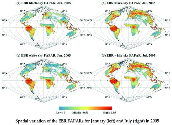
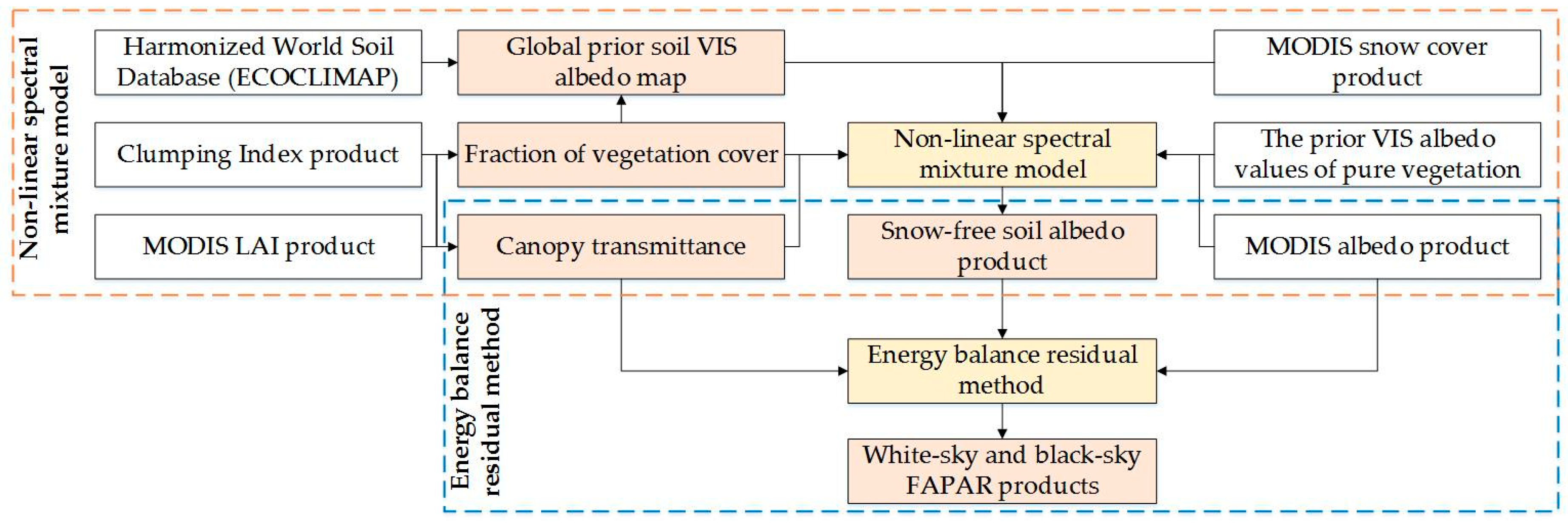
Second, the energy balance residual method was employed to retrieve the white-sky and black-sky FAPAR products based on the MODIS VIS albedo, LAI, CI products, and also the above snow-free soil albedo data. In the EBR method, FAPAR equaled 1 minus the reflected fraction of PAR and the soil-absorbed fraction of PAR. The reflected fraction of PAR was directly provided by the MCD43A3 surface VIS albedo. The soil absorbed fraction of PAR was determined using the canopy transmittance and the retrieved soil VIS albedo using the NSM model. The canopy transmittance was calculated using the gap fraction model based on the MODIS LAI and CI products.

All the prior values needed in the NSM model and EBR method were determined according to the simulations by the PROSAIL model (listed in Table 3) and also the MODIS satellite products.

2.4.1. Estimating White-Sky and Black-Sky FAPAR Using the EBR Method

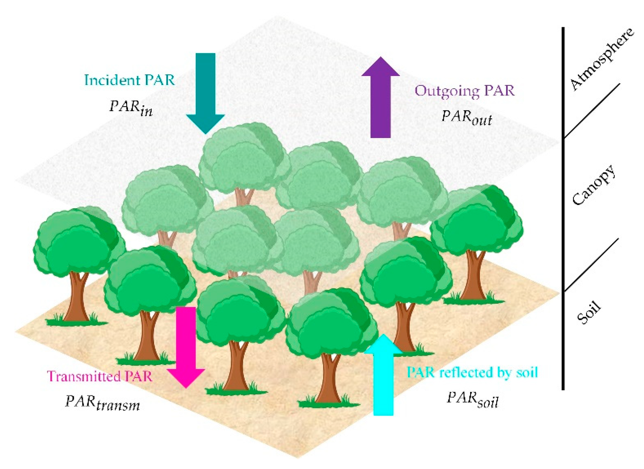
The PAR absorbed by the canopy, $APA{R}_{Canopy}$, excludes the PAR reflected by the canopy and absorbed by the soil background, but includes the small part of PAR absorbed by the canopy after reflection from the underlying background. The energy budget in the soil–canopy–atmosphere structure is shown Figure 2. According to the EBR method, the $APA{R}_{Canopy}$ can be calculated using Equation (1) [5,11,57]:

$${\mathit{APAR}}_{\mathit{canopy}}={\mathit{PAR}}_{\mathit{in}}-{\mathit{PAR}}_{\mathit{out}}-{\mathit{PAR}}_{\mathit{transm}}+{\mathit{PAR}}_{\mathit{soil}}={\mathit{PAR}}_{\mathit{in}}-{\mathit{PAR}}_{\mathit{out}}-{\mathit{APAR}}_{\mathit{Soil}}$$

(1)

where $APA{R}_{canopy}$ and $APA{R}_{soil}$ are the canopy absorbed PAR and soil absorbed PAR, and $PA{R}_{in}$, $PA{R}_{out}$, $PA{R}_{transm}$, and ${\mathit{PAR}}_{\mathit{soil}}$ are the incident PAR, outgoing PAR, transmitted PAR, and PAR reflected by soil substrate, respectively.

Figure 2. The energy budget in the soil–canopy–atmosphere system.

Therefore, FAPAR can be calculated as the ratio of $APA{R}_{Canopy}$ to $PA{R}_{in}$:

$$FAPAR=1-\frac{PA{R}_{out}}{PA{R}_{in}}-\frac{APA{R}_{soil}}{PA{R}_{in}}=1-Albed{o}_{TOC}-Rati{o}_{soil}$$

(2)

where $Albed{o}_{TOC}$, the ratio of $PA{R}_{out}$ to $PA{R}_{in}$, is the VIS albedo of the canopy, which can be directly determined from the MODIS BRDF product: $Rati{o}_{soil}$, the ratio of $APA{R}_{Soil}$ to $PA{R}_{in}$, is the fraction of PAR absorbed by the soil background.

To obtain the canopy FAPAR, it is therefore necessary to derive the $Rati{o}_{soil}$, which can be derived if the canopy transmittance and VIS albedo of the soil background are available. $Rati{o}_{soil}$ can be given by [5,58],

$$Rati{o}_{soil}=\frac{APA{R}_{soil}}{PA{R}_{in}}=\frac{PA{R}_{transm}-PA{R}_{soil}}{PA{R}_{in}}=\frac{PA{R}_{in}\times \tau -PA{R}_{in}\times \tau \times Albed{o}_{soil}}{PA{R}_{in}}=\tau \times \left(1-Albed{o}_{soil}\right)$$

(3)

where $Albed{o}_{soil}$, the ratio of $PA{R}_{soil}$ to $PA{R}_{transm}$, is the VIS albedo of the soil background, and τ is the canopy transmittance.

The canopy directional transmittance, $\tau \left(\theta \right)$, can be determined using the gap fraction model [5,59,60],

$$\tau \left(\theta \right)=e^{-k\times G\left(\theta \right)\times LAI\times CI/\cos \left(\theta \right)}$$

(4)

where $k$ is the leaf extinction coefficient, $G\left(\theta \right)$ is the projection of unit foliage area on the plane perpendicular to the sun incident direction $\theta$, LAI is the leaf area index, CI is the clumping index, and $\theta$ is the SZA. In this paper, the leaf angle distribution was assumed to be a spherical function with $G\left(\theta \right)$ = 0.5. The leaf extinction coefficient $k$ can be determined using the leaf absorptance in the VIS band, which was set as 0.88 according to the simulations using the PROSPECT-5 model and also the measurements of the LOPEX’93 and ANGERS [61].

If the soil background was assumed to be isotropic, the white-sky and black-sky FAPAR can be calculated using Equations (5) and (6):

$$FAPA{R}^{BS}=1-Albed{o}_{Toc}^{BS}-Rati{o}_{soil}^{BS}$$

(5)

$$FAPA{R}^{WS}=1-Albed{o}_{Toc}^{WS}-Rati{o}_{soil}^{WS}$$

(6)

where the superscript $BS$ represents black-sky and $WS$ represents white sky; $Albed{o}_{Toc}^{BS}$ and $Albed{o}_{Toc}^{WS}$ are the black-sky VIS surface albedo and white-sky VIS surface albedo, respectively, which can be directly derived from BRDF products, such as MCD43A3.$Rati{o}_{soil}^{BS}$ and $Rati{o}_{soil}^{WS}$ are the soil-absorbed fraction of PAR under white-sky and black-sky conditions, respectively, and can be determined using Equation (3).

In order to determine $Rati{o}_{soil}^{WS}$, the canopy transmittance under white-sky conditions should be calculated by integrating the directional transmittance $\tau \left(\theta \right)$ over the whole hemisphere:

$${\tau }^{WS}=2\times {\int }_0^{\frac{\pi }{2}}\left(e^{-k\times G\left(\theta \right)\times LAI\times CI/\cos \left(\theta \right)}\right)\times \sin \left(\theta \right)\times \cos \left(\theta \right)d\theta$$

(7)

where ${\tau }^{WS}$ is the canopy transmittance under white-sky condition; other quantities are the same as for Equation (4).

Finally, the total FAPAR can be calculated using a linear combination of the black-sky FAPAR and white-sky FAPAR:

$$FAPA{R}_{Total}=\left(1-Rati{o}_{Sky}\right)\times FAPA{R}^{BS}+Rati{o}_{Sky}\times FAPA{R}^{WS}$$

(8)

where $FAPA{R}_{Total}$ is the total FAPAR and $Rati{o}_{Sky}$ is the proportion of diffuse PAR.

2.4.2. Estimating Snow-Free Soil VIS Albedo Using the Non-Linear Spectral Mixture Model

In the EBR method, the key step is to estimate the VIS albedo of the soil background because the LAI and VIS albedo products are available as part of the MODIS products.

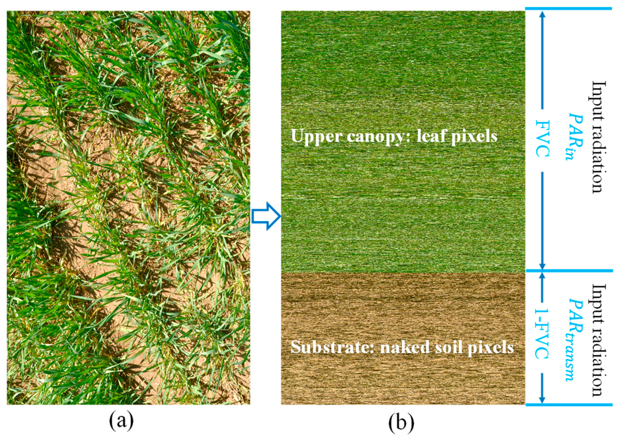
Many methods of analyzing remote sensing data assume that pixels are pure, and so a failure to accommodate mixed pixels may cause significant errors. The linear spectral mixture model, called the patch method, has been widely used to deal with mixed pixels, where each patch (or subpixel) acts independently of the other for the downwelling radiation. However, the linear spectral mixture model or patch method fails to describe mixed pixels for the coupled subpixels: for example, the vegetation canopy and soil background are normally non-linearly mixed due to light interception by the leaves within the upper canopy (see Figure 3a,b).

Figure 3. A physical representation of a non-linear spectral mixture model to simplify the dual-source vegetation–soil lay approach. (a) The vertical digital photo of a wheat canopy; (b) the re-ordered image of (a), in which the leaf and soil pixels are placed side by side in the form of a mosaic. For the soil substrate, its input radiation is attenuated by the leaves of the upper canopy. FVC is the fraction of vegetation cover, $PA{R}_{in}$ and $PA{R}_{transm}$ are the incident and transmitted photosynthetically active radiation, respectively.

In this paper, we employed the layer approach to describe the non-linear contribution of soil background and leaves within the upper canopy on the canopy albedo (Figure 3b). The layer approach was used to account for the contribution of leaves within the upper canopy and soil substrate on the canopy albedo, which treats the upper canopy as semi-transparent for the radiation input [62]. The transmitted PAR above the soil substrate can be determined using Beer’s law,

$$PA{R}_{transm}=PA{R}_{in}\times \tau =PA{R}_{in}\times e^{-k\times G\left(\theta \right)\times LAI\times CI/\cos \left(\theta \right)}$$

(9)

As illustrated in Figure 3b, if all the leaf pixels in Figure 3a were separated and re-ordered together at the upper part, while all the soil pixels were re-ordered at the lower part, a simplified non-linear spectral mixture (NSM) model can be designed to simulate the total canopy albedo by combining the albedo of the “pure” vegetation canopy with an $FVC$ of 100% and soil albedo. For each coarse-resolution pixel, the TOC VIS albedo is approximated as a non-linear mixture of a “pure” vegetation sub-pixel (upper part in Figure 3b with FVC of 100%) and a soil sub-pixel (lower part in Figure 3b):

$$Albed{o}_{TOC}=FVC\times Albed{o}_{pure}+\left(1-FVC\right)\times Albed{o}_{soil}\times \tau$$

(10)

where $Albed{o}_{TOC}$ is the TOC VIS albedo, $FVC$ is the fraction of vegetation cover, $Albed{o}_{pure}$ is the TOC VIS albedo of a “pure” vegetation canopy with an $FVC$ of 100%, $Albed{o}_{soil}$ is the VIS albedo of the soil background, and $\tau$ is the canopy downward transmittance when light is transferred from the TOC to the soil, as in Equation (7). In Equation (10), the canopy VIS albedo is simplified using a weighted mean of the “pure” vegetation subpixel and the soil subpixel; the weighting coefficient used for the soil subpixel is the canopy transmittance.

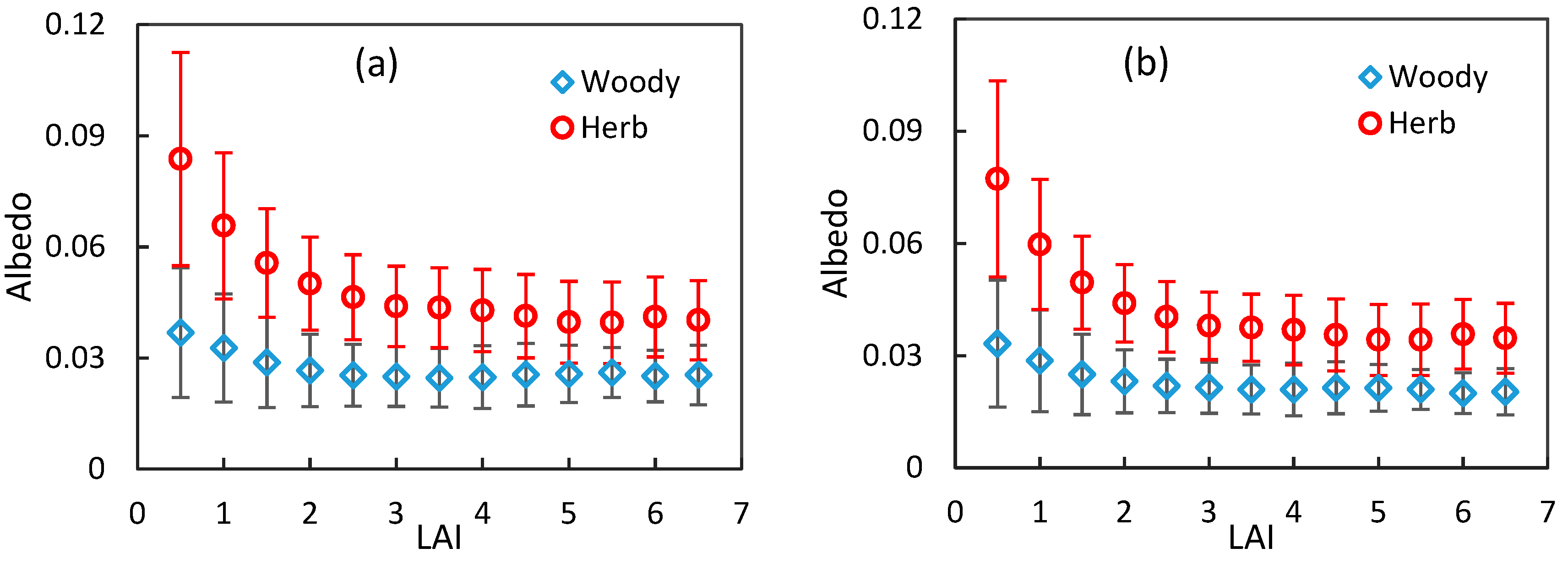
The TOC VIS albedo of “pure” vegetation can be approximated using that of dense vegetation. In this study, we analyzed the TOC VIS albedo for woody and herbaceous vegetation with different LAIs. The VIS albedo data is from the MCD43A3 product, the LAI data is from the MCD15A2H product, and the vegetation types were from the MCD12Q1 product. Only the MODIS products at peak growth stage (during the day of year (DOY) 209–217 in 2005 in the northern hemisphere) was used. For dense canopy, woody cover types, including needleleaf evergreen forest, broadleaf evergreen forest, needleleaf deciduous forest, broadleaf deciduous forest) have almost the same white-sky VIS albedo, while herbaceous vegetation types have a relative higher white-sky VIS albedo. The variations of the white-sky VIS albedo of woody and herbaceous vegetation types with different LAI are illustrated in Figure 4. The VIS albedo decreased with increased LAI, and became quite stable when LAI was greater than four. Therefore, we assumed that the VIS albedo for pure vegetation can be represented by the VIS albedo for vegetation with a “saturated” LAI value (e.g., LAI = 6). So, the priori VIS albedo values of “pure” vegetation with an FVC of 100 were designated as 0.025 and 0.041 for white-sky albedo of woody and herbaceous vegetation types, and 0.020 and 0.036 for black-sky albedo, respectively, which is corresponding to the VIS albedo of a dense canopy with an LAI value of 6.

Figure 4. Variations of the white-sky (a) and black-sky (b) VIS albedo of woody vegetation and herbaceous vegetation with different LAI. The error bar is the standard deviation.

$\mathrm{The} FVC$ can also be calculated using the gap fraction model with a fixed SZA of 0° and a fixed leaf extinction coefficient of 1:

$$FVC=1-e^{-G\left(\theta \right)\times LAI\times CI}$$

(11)

The canopy transmittance and $FVC$ can, therefore, be determined using LAI and CI data. The VIS albedo of the soil background can then be retrieved using the NSM model:

$$Albed{o}_{soil}=\frac{Albed{o}_{TOC}-FVC\times Albed{o}_{pure}}{\left(1-FVC\right)\times \tau }$$

(12)

Here, the TOC VIS albedo can be directly derived from the MCD43A3 BRDF products, and FVC and $\tau$ can be determined using Equations (11) and (7), respectively. In this paper, the soil substrate was assumed as isotropic, and only the white-sky albedo of soil substrate was calculated.

If the NSM model shown in Equation (12) was employed to retrieve the soil VIS albedo, the uncertainty for dense vegetation pixels would be very large. For example, the error in the canopy VIS albedo will be magnified by about 100 times for a vegetation canopy with an $FVC$ of 0.9, because the denominator of Equation (12) is then about 0.01. In order to address this problem, the abnormal soil VIS albedos obtained using the NSM model were replaced by the prior values. These prior values of soil VIS albedo can be determined using the yearly composite values, or be approximated using empirical formulae based on the soil organic deposition and texture of the soil [55]. The ECOCLIMAP (a global database of land surface parameters at 1 km resolution) uses an empirical equation to calculate soil reflectance, as given in Carrer et al. [56],

$$Albed{o}_{soil}=0.1+\left(0.05+0.3\ast f_{sand}\right)\times (1-0.9\times FV{C}^2)$$

(13)

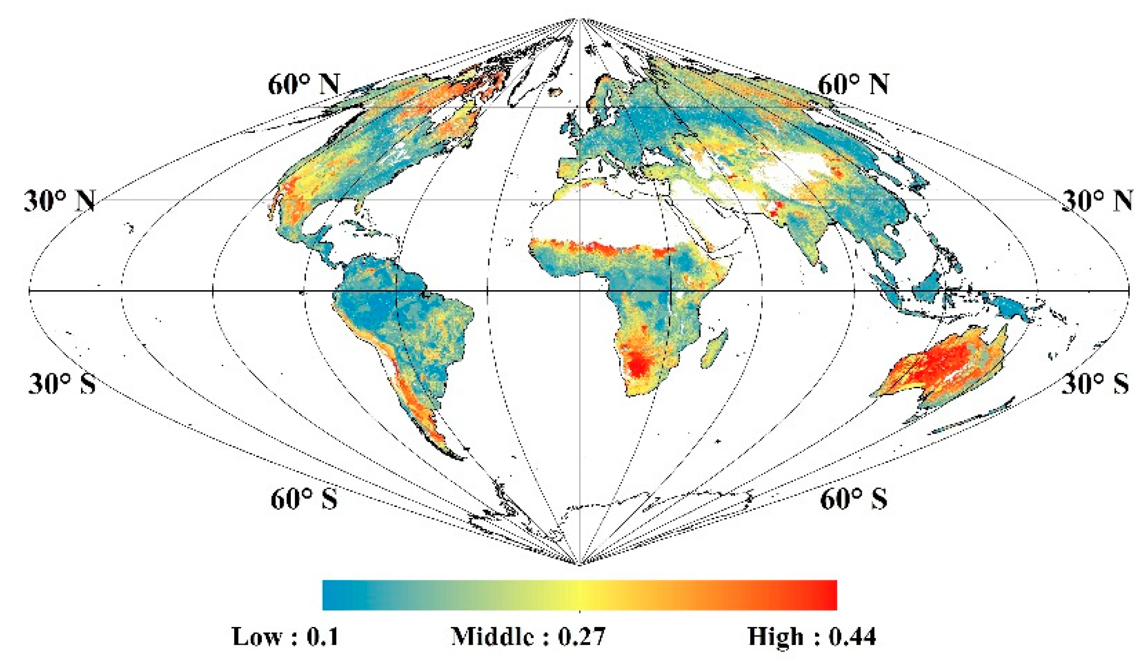
where $f_{sand}$ is the sand fraction. The global sand fraction data are derived from the Harmonized World Soil Database (FAO/IIASA/ISRIC/ISSCAS/JRC, 2009). The prior soil VIS albedo was mapped using the ECOCLIMAP sand fraction data and the yearly maximum FVC values derived from the MODIS CI and MCD15A2H LAI products based on the gap fraction model (Equation (11)), as shown in Figure 5.

Figure 5. The global prior soil VIS albedo map obtained using the ECOCLIMAP sand fraction data and the yearly maximum FVC values derived from the MCD15A2H product and gap fraction model.

In this study, if the retrieved soil VIS albedo value was smaller than 0.02 or greater than 0.3 (the two threshold values given in Myneni et al. [3] and Equation (13)) for snow-free pixels with an FVC > 0.3, the pixels were marked as abnormal and their soil VIS albedo values were replaced either by the yearly composite value (if there were more than three valid retrievals within a year) or the prior values determined by substituting the sand fraction and FVC values in Equation (13).

The TOC VIS albedo of a “pure” vegetation canopy will increase greatly if it is covered by snow and the NSM model will then fail to estimate the VIS soil albedo. For pixels determined to be snow-covered by the MOD10A2 snow cover product, the canopy black-sky FAPAR was directly determined using the gap fraction method as used in Xiao et al. [21], where the black-sky FAPAR was assumed equal to one minus the canopy directional transmittance ($\tau \left(\theta \right)$) as Equation (4); then, the canopy diffuse transmittance, ${\tau }^{WS}$, was calculated by integrating $\tau \left(\theta \right)$ over the whole hemisphere (as Equation (7)) to determine the white-sky FAPAR ($1-{\tau }^{WS}$).

Furthermore, in some regions, such as boreal forest, the soil surface is typically covered by different understory species (including litter, moss, lichen, etc.). Such cases were not taken into account in the NSM model. We did not discriminate the understory vegetation from soil background, and the soil albedo was regarded as the understory albedo for the forest region.

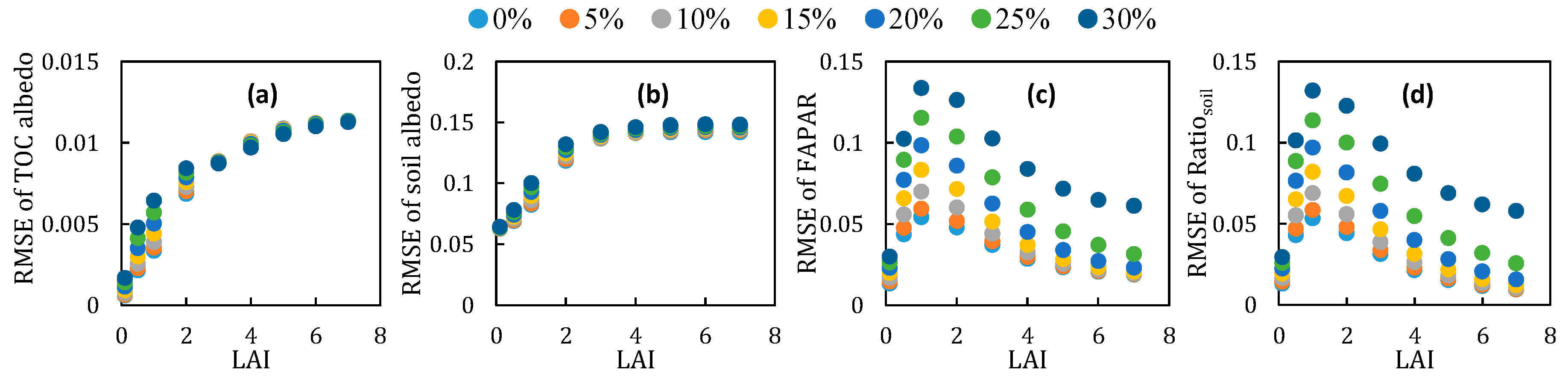
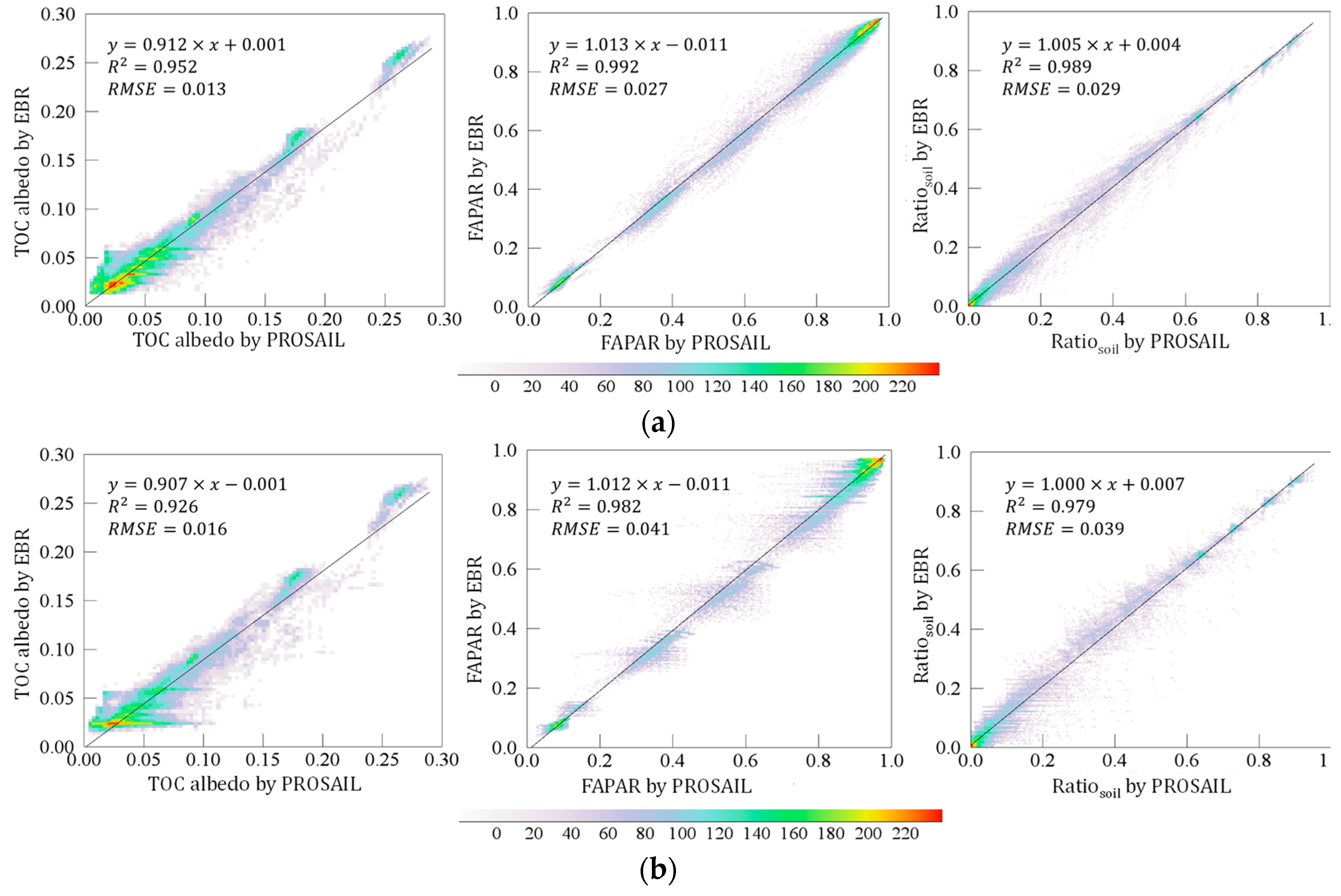
However, there was no in situ dataset to validate the VIS albedo of soil substrate at 500 m resolution. So, the simulations by the PROSAIL model were treated as the “true” values to indirectly validate the NSM model and EBR method. Furthermore, in order to quantify the sensitivity of the NSM model and EBR method, a Gaussian random noise with a relative intensity of 0% to 30% was added to the canopy LAI values. One-thousand different random noises were added to each of the 81,000 simulated samples listed in Table 4.

Table 4. The main inputs of the NSM model and EBR method in the validation experiment using simulations by the PROSAIL model. A Gaussian random noise with a relative intensity of 0% to 30% was added to the canopy LAI values to investigate the sensitivity of the EBR approach.

Parameter	Definition	Units	Range or Values
Leaf optical
k	Leaf extinction coefficient, varies with leaf chlorophyll content (Cab)	-	0.88
Canopy
LAI	Leaf area index	m2/m2	0.1, 0.5, 1, 2, 3, 4, 5, 6, 7
LAI noise	Gaussian random noise	-	0%, 5%, 10%, 15%, 20%, 25%, 30% of the “true” LAI
G(θ)	The projection of unit foliage area on the plane perpendicular to the sun incident direction θ	-	0.5
CI	clumping index	-	1
${\mathit{Albedo}}_{\mathit{pure}}$	VIS albedo of “pure” vegetation	-	0.025
Soil
$Albed{o}_{soil}$	Hemisphere reflectance, assumed as isotropic	-	Limited to 0.02–0.3
Remote sensing data
$Albed{o}_{TOC}$	TOC VIS white-sky and black-sky albedo	-	81,000 simulations by PROSAIL shown in Table 3
Imaging Geometry, same as Table 3
SZA	Sun zenith angle	degrees	10, 30, 45, 60, 75
$Rati{o}_{Sky}$	Ratio of diffuse light	-	0.3, 0.5, 0.7

3. Results

3.1. Validation Using Simulations by PROSAIL

The 81,000 simulations made using the PROSAIL model (see Table 3 for details) were used to validate the NSM model VIS albedo and the EBR method.

Figure 6 illustrates the validation results for the VIS canopy albedo, the fraction of PAR absorbed by the soil, and the canopy FAPAR. For the simulated dataset by PROSAIL, the “true” values of the leaf extinction coefficient (k), G(θ), and $Albed{o}_{pure}$ needed in the NSM model and EBR can be accurately determined for each specific sample. However, these parameters are not available for generating global FAPAR products. So we evaluated the performance of the NSM model and EBR method with both “true” values (Figure 6a) and fixed values (Figure 6b) of k, G(θ), and $Albed{o}_{pure}$. The results show that, the NSM model and EBR method can give more accurate retrievals with “true” values of the parameters. With fixed values (k = 0.88, G(θ) = 0.5, $Albed{o}_{pure}$ = 0.025), the VIS canopy albedo and soil-absorbed fraction of PAR can be still accurately modeled using the NSM model—the results give the RMSEs of 0.016 and 0.039, respectively. In addition, the canopy FAPAR can also be accurately estimated using the EBR method; in this case, the RMSE as 0.041 and R² was 0.982. Therefore, if the LAI can be accurately estimated using remote sensing data, it should be possible to calculate the FAPAR accurately using the remotely sensed canopy VIS albedo even if the variations in the TOC VIS albedo of the “pure” vegetation ($Albed{o}_{pure}$), the leaf extinction coefficient (k), and also the $G\left(\theta \right)$ are neglected.

Figure 6. Evaluation of the EBR approach using the 81,000 simulations by PROSAIL. (a) “True” values of the leaf extinction coefficient (k), $Albed{o}_{pure}$, and G(θ) were available from PROSAIL simulations, (b) the prior parameters were fixed (k = 0.88, G(θ) = 0.5, $Albed{o}_{pure}$ = 0.025).

The sensitivity of the EBR method was also investigated using the noised-LAI dataset (assumed a random noise existing in the LAI products) as illustrated in Figure 7. The results show that the EBR method gives robust and accurate estimation of the canopy VIS albedo, FAPAR, and soil absorbed fraction of PAR, with a RMSE less than 0.012, 0.133, and 0.132, respectively, if the noise of the LAI data was smaller than 30%. The FAPAR can be more accurately estimated for both sparse (LAI < 1) and dense canopies (LAI ≥ 2)—the largest RMSE was for a vegetation canopy with an LAI value of 1.

Figure 7. The mean RMSE of the retrieved TOC VIS albedo, soil VIS albedo, FAPAR, and soil-absorbed fraction of PAR using the EBR method for the 81,000 simulations with a Gaussian random noise in the LAI values (0% to 30%). Figures (a–d) correspond to the TOC VIS albedo, soil VIS albedo, FAPAR, and soil-absorbed fraction of PAR, respectively.

However, the retrieval error of soil VIS albedo increases rapidly when the LAI increases (Figure 7b). Here, the soil VIS albedo was forcibly limited to the range 0.02–0.3. Almost all the retrieved soil VIS albedos fall into wrong range if the LAI is greater than three, so the RMSE value of the retrieved VIS soil albedo in Figure 7b was almost same when LAI was greater than three. The results show that the soil VIS albedo can be accurately retrieved with an RMSE value < 0.05 for sparse vegetation (LAI < 1).

3.2. Global Snow-Free VIS Soil Albedo

The global VIS soil albedo and the temporal variations in the VIS albedo were calculated from the MCD43A3 VIS albedo product and MCD15A2H LAI product using the NSM model shown in Equation (12). Figure 8 shows the global map of the yearly-averaged snow-free VIS albedo of the soil background (the mean value of all the valid retrievals using Equation (12)) and the number of valid retrievals for 2005. The retrieved VIS soil albedo was high in deserts and in regions where there is sparse grass, including the Sahara Desert, inland Australia, and the Eurasian Steppe region, whereas it was low in the tropical forest regions of Southeast Asia, the Amazon Basin, and the African Congo Basin. The number of valid retrievals of the VIS soil albedo was high in regions of sparse vegetation and low in regions of dense vegetation, especially in tropical forest regions. The yearly mean values of the retrieved VIS soil albedo for different vegetation types in Figure 8 were summarized in Table 5.

Figure 8. Global maps of the yearly snow-free VIS soil albedo (a) and the number of valid retrievals in 2005 (b).

Table 5. The yearly mean values of the snow-free soil VIS albedo retrieved using the NSM model for different vegetation types in 2005.

Type	NLE	BLE	NLD	BLD	Shru	Sav	GCC	BLC	MF	CNM
Albedo	0.069	0.120	0.085	0.120	0.109	0.111	0.144	0.134	0.109	0.120

NLE: needleleaf evergreen forest, BLE: broad-leaf evergreen forest, NLD: needleleaf deciduous forest, BLD: broadleaf deciduous forest, Shru: shrublands, Sav: savannas, GCC: grasses and cereal crop, BLCs: broadleaf crops, MF: mixed forest, CNM: crop/natural vegetation mosaic.

Figure 9 shows the global effective retrieval fraction for VIS soil albedo values derived using the NSM model in 2005. The results indicate that about 58–75% of snow-free pixels can have their VIS albedo inverted from the MODIS VIS albedo products. The VIS soil albedo retrieval fraction decreases noticeably in winter due to snow cover and also decreases slightly in the peak summer growth season.

Figure 9. The global effective retrieval fraction for VIS soil albedo derived using the NSM model with MODIS products in 2005. If the retrieved soil VIS albedo was smaller than 0.02 or greater than 0.3 for a snow-free pixel with an FVC > 0.3, the pixel was marked as abnormal.

The yearly mean values of the VIS soil albedo in 2005 retrieved using the NSM model for the different vegetation types listed in Table 5 were linked to the ECOCLIMAP soil albedo data, and the statistical result shows a strong linear relationship between the two soil albedo datasets (y = 0.536x + 0.025, R² = 0.860).

3.3. EBR FAPAR Validation Using VALERI Sites

A statistical analysis was conducted to examine the relationship between the retrieved black-sky FAPAR at 10:30 and white-sky FAPAR using VALERI site locations. The results showed that there was a linear relationship between the white-sky FAPAR and black-sky FAPAR at 10:30 (y = 1.062x + 0.024, R² = 0.995), and that the white-sky FAPAR is a little higher than the black-sky FAPAR.

Next, the black-sky FAPAR retrieved using the EBR method was compared to the MCD15A2H and GEOV1 FAPARs. Results showed that the EBR black-sky FAPAR was more accurate (R² = 0.917, RMSE = 0.088, and bias = -2.8 %) than MCD15A2H (R² = 0.901, RMSE = 0.096, and bias =7.6 %) and GEOV1 (R² = 0.868, RMSE = 0.105, and bias = 6.1%) (Figure 10, Table 6.).

Figure 10. Validation of the EBR black-sky FAPAR (EBR^BS), MCD15A2H, and GEOV1 FAPAR products using reference FAPAR estimates from 22 VALERI sites.

The quantitative accuracy assessment for the FAPAR products are shown in Table 6. The results for herbaceous and woody vegetation were also analyzed separately, as shown in Table 6b,c. The results show that for herbaceous vegetation, the black-sky FAPAR obtained using the EBR method was slightly lower than the measured FAPAR (7.2% underestimation), while for woody vegetation, the black-sky FAPAR obtained using the EBR method was very slightly overestimated (0.1%). For both types of vegetation, the white-sky FAPAR was slightly overestimated (7.5% for herbaceous vegetation, 10.8% for woody vegetation, and 9.5% for all samples); In general, the EBR black-sky FAPAR gave the best unbiased estimation, with a bias of about −2.8% against 7.6% for MCD15A2H and 6.1% for GEOV1.

3.4. Spatio-Temporal Variation of the FAPAR Products

To investigate spatial patterns specific to a given FAPAR product, global maps of the monthly mean values for the MCD15A2H, GEOV1, EBR black-sky, and white-sky FAPAR products were calculated for January and July in 2005. All FAPAR datasets exhibited similar spatial patterns and seasonal variations (Figure 11). Higher FAPAR values were distributed over equatorial forest regions and boreal forest regions around 50–60°N in July, and over equatorial forest regions in January.

Figure 11. Spatial variation of the monthly mean FAPARs for January (left) and July (right) in 2005: (a–b) EBR method-based black-sky FAPARs; (c–d) EBR method-based white-sky FAPARs; (e–f) MCD15A2H FAPARs; and (g–h) GEOV1 FAPARs.

However, discrepancies were evident in the scatterplots of the FAPAR products (Figure 12). The EBR white-sky FAPAR was higher than the black-sky FAPAR when the SZA was less than T0 (about 60°) for most observations at middle and low latitudes. The MOD15A2H2 FAPAR gave an obvious overestimate compared to the EBR black-sky FAPAR. The GEOV1 FAPAR produced an obvious overestimate compared to the EBR black-sky FAPAR except for canopies with very small FAPAR values (<0.2)—it also gave a noticeable underestimate for canopies with very small FAPAR values (<0.2) if compared to the EBR white-sky FAPAR. The EBR white-sky FAPAR agreed better than the EBR black-sky FAPAR with the MCD15A2H and GEOV1 FAPARs. The MCD15A2H FAPAR agreed better than the GEOV1 FAPAR with the EBR black-sky and white-sky FAPARs. Lastly, we could find a “horizontal red line” over high FAPAR regions in Figure 12a,b, which indicates “abnormal” pixels in the MODIS FAPAR products. These ‘abnormal’ pixels were mainly located in the high LAI value areas (with a mean value of 6.32 and standard deviation value of 0.71). The MCD15A2H FAPAR retrieved algorithm suffered from the “saturation phenomenon’” over the high LAI areas [63], so the MCD15A2H FAPAR kept stable while the EBR FAPAR varied over the high values.

Figure 12. Comparison of FAPAR estimates for July 2005: (a–b) EBR black-sky and white-sky FAPARs against MOD15A2H FAPAR; (c–d) EBR black-sky and white-sky FAPARs against GEOV1 FAPAR; and (e) EBR black-sky FAPAR against EBR white-sky FAPAR (Note that the Sun Zenith Angle (SZA) threshold value (T0) was approximately 60).

3.5. Seasonal Variation of the FAPAR Products

Figure 13 illustrates the seasonal variations in the FAPAR for different vegetation types within tile H10V05 in 2005. The EBR black-sky FAPAR was smaller than the white-sky FAPAR outside the winter season with the large SZA. The EBR white-sky FAPAR agreed well with the MODIS FAPAR but was smaller than the MODIS FAPAR in the spring and winter seasons. The EBR black-sky FAPAR was noticeably smaller than the MODIS FAPAR for all land cover types. The GEOV1 and MODIS FAPARs agreed with the EBR white-sky FAPAR at broadleaf deciduous forests, savannas, grasslands, and croplands. For these biomes, the EBR black-sky FAPARs were notably lower than the other FAPAR estimates. However, the EBR black-sky FAPAR agreed well with the GEOV1 for needleleaf forests and shrublands.

Figure 13. Time-series of the mean of the EBR black-sky, EBR white sky, MCD15A2H, and GEOV1 FAPARs of different vegetation types within tile H10V05 (located in North America, covering 30.0°N–40.0°N and 80.0°W–104.4°W) for 2005.

4. Discussion

4.1. Limitations of the Gap Fraction Model and NSM Model

In this study, the gap fraction model and MODIS LAI (MCD15A2H) were employed to determine the canopy transmittance in the EBR method. The MODIS LAI was based on the inversion of the 3D radiative transfer model [15], which describes global vegetation using biomes, which are characterized by variables such as clumping, soil, reflectance, and stem ratio [3,15]. In the gap fraction model, only the LAI and leaf clumping effect are considered, and the woody components’ (branches, stems) influence on the canopy transmittance is neglected. The woody components contribute extra radiation absorption in the forest canopy. Therefore, the canopy transmittance using the gap fraction model may be overestimated for forest regions, which can affect the retrieval of soil albedo and soil absorbed fraction of PAR. Chen et al. [5,64] introduced the needle-to-shoot ratio and woody area index to address this problem. If the prior data concerning the needle-to-shoot ratio and woody area index are available, the gap fraction model can be improved to give a more accurate estimation of the canopy transmittance for forest regions [64].

The multiple scattering within the canopy is also neglected when the canopy transmittance is approximated using the gap fraction method (Equation (4)). This approximation has also been widely employed by other researchers (for example, Xiao et al. [21], for the GLASS FAPAR product). In the VIS band, the leaf single scattering albedo is low (it was fixed as 0.12 in this study), and this approximation introduces a degree of error in determining of canopy transmittance. So, the multiple scattering within the canopy will result in some errors when the gap fraction method is employed in the NSM model and EBR method. The NSM model, which does not account for multiple scattering effects, gave a small RMSE (of 0.028) for the canopy FAPAR as it was validated using PROSAIL simulations, which account for multiple scattering effects. Therefore, the error produced by the EBR method was very small even though the multiple scattering was neglected.

Furthermore, the NSM model, a simplified layer approach, was employed to simplify the dual-source vegetation–soil transfer models, such as PROSAIL [53], four-scale [65], and KUUSK [66]. This layer approach, which treats the upper canopy as semi-transparent for the radiation input, may not work for clumped or patchy vegetation, in which both the canopy and the bare soil are uncoupled, and receive full radiation loading [62]. For such an uncoupled dual-source case, the linear spectral mixture model, or the combination of the NSM model and the linear spectral mixture model may be more effective to deal with such mixed pixels with coarse resolution if the percentage of the patchy-distributed vegetation is available.

4.2. Directional Effect of the Clumping Index and Its Influence on the Retrieval of FAPAR

To characterize the clumping effects of leaves within a canopy, Nilson [59] added a vegetation dispersion parameter ($\mathsf{\Omega }$) to the directional gap fraction model:

$$P\left(\theta \right)=exp\left(-G\left(\theta \right)\times LAI\times \mathsf{\Omega }\left(\theta \right)/cos\left(\theta \right)\right)$$

(14)

where $\theta$ is the zenith angle, $P$ is the gap probability, $\mathsf{\Omega }\left(\theta \right)$ is the directional clumping index, and $G\left(\theta \right)$ is the foliage area orientation function (i.e., the G-function).

To avoid the variation in the clumping index as a function of $\theta$, an average clumping index (CI) was proposed by Chen et al. [43] through a definition using the effective LAI ($LA{I}_e$) [43]:

$$CI=LA{I}_e/LAI$$

(15)

where $LA{I}_e$ can be computed using the following formula [5]:

$$LA{I}_e=-2{\int }_0^{\frac{\pi }{2}}\ln \left(P\left(\theta \right)\right)\times cos\left(\theta \right)\times sin\left(\theta \right))d\theta$$

(16)

In this study, the CI product by Jiao et al. [38], as defined in Equation (15), was used to calculate both the black-sky and white-sky FAPARs. Thus, using an averaged CI is reasonable when calculating the white-sky transmittance whereas the directional CI, $\mathsf{\Omega }\left(\theta \right)$, should be employed to calculate the black-sky transmittance.

The directional clumping index, $\mathsf{\Omega }\left(\theta \right)$, generally increases with increasing zenith angle [43,67]. According to simulations and observations, $\mathsf{\Omega }\left(\theta \right)$ may increase by about 20%–30% for some vegetation types, such as crop and forest, if the zenith angle increases from 30° to 80° [43,60,65,67,68]. However, there is no directional CI product available. Therefore, the black-sky transmittance and FAPAR may be overestimated for solar illumination with a small SZA, and under-estimated for illumination with a large SZA. More attention should be paid to investigate the directional effects of the clumping index and to examine its influence on the retrieval of canopy black-sky FAPAR.

5. Conclusions

This paper presented an EBR method for producing a VIS global soil background albedo, as well as white-sky and black-sky FAPAR datasets using MODIS broadband albedo together with the LAI and CI product.

An NSM model was proposed to simulate the TOC albedo and also to retrieve VIS soil albedo. According to the validation with PROSAIL simulations, the NSM model have an RMSE of 0.015 and an R² value of 0.932 for the TOC VIS albedo, and the EBR method gave an RMSE of 0.039 and an R² of 0.984 for FAPAR. Direct validation against observations at VALERI sites demonstrated that the EBR black-sky FAPAR product was more accurate and unbiased (R² = 0.917, RMSE = 0.088, and bias =−2.8 %) than the GEOV1 (R² = 0.868, RMSE = 0.105, and bias = 6.1%) and MCD15A2H (R² = 0.901, RMSE = 0.096, and bias = 7.6 %) products.

This study provided a new global white-sky and black-sky FAPAR dataset, just like MCD43A3 albedo product, for the remote sensing community. The two FAPAR products and the soil VIS albedo product are available at http://www.geodata.cn/.