Time-Series InSAR Monitoring of Permafrost Freeze-Thaw Seasonal Displacement over Qinghai–Tibetan Plateau Using Sentinel-1 Data

Abstract

Permafrost is widely distributed in the Tibetan Plateau. Seasonal freeze–thaw cycles of permafrost result in upward and downward surface displacement. Multitemporal interferometric synthetic aperture radar (MT-InSAR) observations provide an effective method for monitoring permafrost displacement under difficult terrain and climatic conditions. In this study, a seasonal sinusoidal model-based new small baselines subset (NSBAS) chain was adopted to obtain a deformation time series. An experimental study was carried out using 33 scenes of Sentinel-1 data (S-1) from 28 November 2017 to 29 December 2018 with frequent revisit (12 days) observations. The spatial and temporal characteristics of the surface displacements variation combined with different types of surface land cover, elevation and surface temperature factors were analyzed. The results revealed that the seasonal changes observed in the time series of ground movements, induced by freeze–thaw cycles were observed on flat surfaces of sedimentary basins and mountainous areas with gentle slopes. The estimated seasonal oscillations ranged from 2 mm to 30 mm, which were smaller in Alpine deserts than in Alpine meadows. In particular, there were significant systematic differences in seasonal surface deformation between areas near mountains and sedimentary basins. It was also found that the time series of deformation was consistent with the variation of surface temperature. Based on soil moisture active/passive (SMAP) L4 surface and root zone soil moisture data, the deformation analysis influenced by soil moisture factors was also carried out. The comprehensive analysis of deformation results and auxiliary data (elevation, soil moisture and surface temperature et al.) provides important insights for the monitoring of the seasonal freeze-thaw cycles in the Tibetan Plateau.

1. Introduction

The Qinghai–Tibetan Plateau (QTP) is the largest area with permafrost outside the polar regions, occupying up to 50% of the plateau [1]. The upper layer of the permafrost is overlain by an active layer that undergoes seasonal freezing and thawing [2]. The amplitude of the surface uplift or subsidence varies spatially and temporally, scaling with the active layer thickness (ALT) and water–ice phase [3]. Time-series measurements of surface deformation of permafrost are of great significance for assessing the displacement response of seasonal variations and environmental factors, mitigating geohazards and climate change, and planning future land use.

In the past two decades, various studies have been successfully conducted to map and investigate natural environment surface displacements of permafrost areas [4,5,6,7,8]. Those studies have focused on the selection of SAR interferometry (InSAR) method, seasonal displacement model, SAR band selection, etc. For example, Liu et al. [9] applied InSAR to measure surface deformation over permafrost on the North Slope of Alaska during thawing season. Antonova et al. [10] measured seasonal and multiyear ground movements in a yedoma region of the Lena River Delta, Siberia. Two studies (Wolfe et al. and Beck et al. [6,7]) investigated the permafrost terrain stability by the differential InSAR (DInSAR) method. Two other studies Short et al. and Wang et al. [2,4] compared the performance of TerraSAR-X, ALOS PALSAR and RADARSAT-2 data in monitoring ground displacement over continuous and discontinuous permafrost regions. To assess surface deformation over QTP, a number of studies have reported a centimeter-scale seasonal and multiyear isotropic thaw subsidence and freezing uplift in permafrost areas with different scales by DInSAR [2,5,8] or multitemporal interferometric synthetic aperture radar (MT-InSAR) methods [11,12,13,14]. High-resolution images, such as TerraSAR-X and COSMO-SkyMed, can greatly improve the level of the details compared with medium-resolution SAR images, and can monitor the detailed displacement of man-made features such as railway and highway [10,13,14,15,16]. However, those studies are done in limited study areas and are susceptible to serious temporal decorrelation due to the short wavelength. Hence, some studies also focused on the surface deformation in QTP permafrost in regional scale [3,11,17,18]. For example, Daout et al. [3] retrieved the permafrost related deformation through the entire seasonal cycle over a wide area with long temporal range (2003–2011).

Due to the global and seasonal temperature changes, without dominant scatter and phase variation, the backscattering and phase features of the ground targets in the permafrost region are significantly affected by spatial-temporal decorrelation, which obscures the underlying signal and limits the application of InSAR [19,20]. To reduce and overcome those limitations, MT-InSAR methods, including small baselines subset (SBAS) techniques [21], persistent scatter interferometry (PSI) techniques [22,23,24], and other PSI- and SBAS-like methods (Stanford method for persistent scatters (StaMPS) [19], temporally coherent point InSAR (TCP-InSAR) [25,26,27]) have been applied to numerous examples of surface displacement [12,28,29,30]. Compared with conventional InSAR methods, MT-InSAR shows better performance in urban environments. However, in mountainous or plateau permafrost regions, the MT-InSAR method is restricted by the decorrelation or insufficient coherence points created by cryoturbation of the surface, steep terrains, dense vegetation and snow/ice cover in winter [31]. To overcome those shortcomings, methods have been proposed that explore distributed scatterers (DS) [32], quasi-persistent scatterers (QPS) [33] and temporarily coherent points (TCPs) [34]. In addition, in MT-InSAR methods, the linear deformation model cannot properly describe the deformation processes of permafrost, which will result in large estimation error. To overcome those limitations, choosing the appropriate seasonal deformation model is crucial to MT-InSAR analysis over permafrost. For example, Liu et al. [9] proposed a simplified Stefan model-based season deformation model, which took the settlement accumulation time during the thawing of frozen soil into consideration. Others, Zhao et al. [12] considered the climatic factors, tectonic activities and thermal characteristics of frozen soil in surface deformation modeling. Another group, Dong et al. [35], simulated the common sinusoidal approximation model of ground deformation due to annual and biannual seasonal variations, which is capable of mapping those variations and parameterizing known and unknown nonlinear processes.

In this paper, the new SBAS (NSBAS) technique with a sinusoidal seasonal model is developed to monitor freeze–thaw seasonal displacement of QTP. Unlike Stefan [9] or other climatic factor-dependent seasonal models, the sinusoidal model does not need to prepare auxiliary data for modeling. It is a better choice for seasonal displacement estimation when climatic data are not available. To understand the spatial patterns of seasonal displacement in detail and reduce the temporal decorrelation effects, a total of 33 S-1 images taken at intervals as short as 12 days from 28 November 2017 to 29 December 2018 were collected to build the MT-InSAR analyzing network. The seasonal oscillations of QTP under different land cover types were discussed and analyzed in detail. To describe seasonal oscillations more accurately, high resolution TerraSAR-X images were used to distinguish land cover. We carried out the evaluation and comparison of seasonal displacement variation and influencing factor analysis of different surface features corresponding to surface temperature data (SMAP L4 surface temperature product), soil moisture data (SMAP L4 surface/root zone soil moisture products), elevation, slope and in situ ALT. The cross-correlations between time-series displacement and processes involved in the freeze-thaw cycle and permafrost evolution are also discussed.

2. Study Area and Datasets

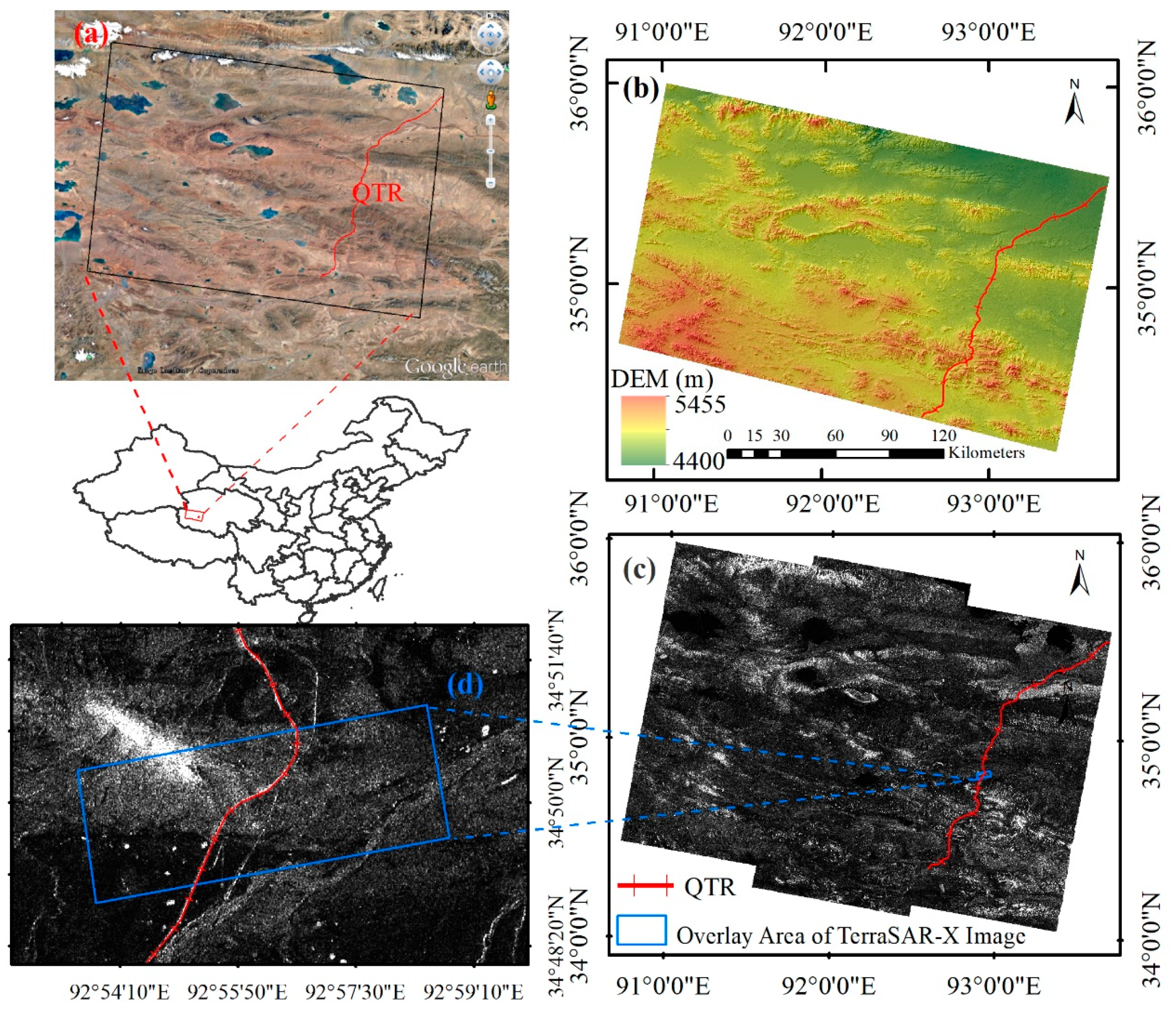
2.1. Study Area

The study area was located in the south of Qinghai province (longitude: 90.715−93.751, latitude: 34.204−35.836), covering an area of about 37440 km² (Figure 1a). The elevation ranges from 4400 to 5455 m (Figure 1b). The QTR across our study area is about 221 km long, accounting for about 20% of total QTR. The QTR in high altitude areas is significantly impacted by the permafrost environment. According to the Google Map (Figure 1a) and a TerraSAR-X amplitude image (Figure 1d), the land cover is classified into three types, i.e., alpine steppe, barren, and alpine meadow [36]. The study area experiences a continental climate characterized by extremely cold and dry winters, warm and humid summers with plenty of rain, and the maximum and minimum air temperatures of 23 and −38 °C, respectively [36]. The annual precipitation ranges from 50 to 400 mm, due to cold and arid environment.

2.2. Dataset

2.2.1. Sentinel-1 Data

We collected 33 descending Sentinel-1A images from 28 November, 2017 to 29 December, 2018, which covered the entire seasonal cycle for MT-InSAR analysis. All of the Sentinel-1A scenes used in this study were VV-polarized with incidence angles of approximately 39.5°. The ranges of perpendicular baseline were from −59.77 to 77.22.

2.2.2. Ancillary Data

In this study, some auxiliary data were also used to analyze the results of MT-InSAR. A scene of High-resolution TerraSAR-X image (11 December 2015) was used to acquire high precision land cover classification, detailed description of the TerraSAR-X data can be found in [36]. We derived the SMAP level 4 daily surface temperature and surface/root zone soil moisture products from National Aeronautics and Space Administration (NASA), distributed over a 9 km grid. These data are available at https://nsidc.org/. The introduction of those data were shown in [37]. The time series distribution of those products from 28 November, 2017 to 29 December, 2018 was extracted. Ground-penetrating radar (GPR) has been widely used in detecting shallow underground conditions of permafrost, such as ALT over polar and mountainous areas [38]. The in situ ALT data were measured by GPR in August 28, 2018. The electromagnetic characteristics of stratum was collected using LTD-2100, detailed introduction of the instrument can be found in [39], the collected data were processed based on software IDSP5.0 (China Research Institute of Radiowave Propagation (CRIRP), Xinxiang, China), subsequently.

3. Methodology

In the QTP area, the surface displacement shows obvious seasonal variation. It was worth exploring an effective procedure to evaluate the deformation of permafrost in more detail. The objective of this study was to monitor the freeze-thaw seasonal displacement of QTP based on MT-InSAR. The processing flow chart consists of four main steps: 1) InSAR processing of the images, including preprocessing (interferogram network selection, co-registration, differential interferogram phase generation, phase unwrapping) and phase correction; 2) seasonal displacement modeling; 3) NSBAS deformation estimation; 4) spatial variation analysis of seasonal oscillation amplitude and time-series variation analysis of deformation based on auxiliary data. An overview of the methodology is illustrated in Figure 2, and the detailed steps are as follows.

3.1. InSAR Processing

In our study area, the permafrost nature surface experiences seasonal dynamic changes caused by vegetation, which contributes to spatial-temporal decorrelation. To accommodate this limitation, it was necessary to adjust the set of interferogram pairs based on spatial-temporal baseline distribution and coherence. After all the SAR images were co-registered, with perpendicular baseline < 100 m and temporal baseline < 40 days, and the interferograms in fine coherence were checked and selected, a total of 77 interferometric pairs were used to generate interferograms. They allowed us to monitor the deformation in short time intervals through the year.

The topographic phase was removed from the observed interferometric phase using the 1-arcsecond grid (30 m) shuttle radar topography mission (SRTM) digital elevation model (DEM) [40]. The phase term from noise was removed by means of adaptive filtering and multilooking (the averaging of two pixels in range and 10 pixels in azimuth). After removing or reducing the topography and noise phase, the remaining phase was mainly related to ground deformation, atmospheric and orbital errors. A minimum cost flow (MCF) phase unwrap technique [41] was used for unwrapping the phase. We generated the unwrapped interferograms for the selected image pairs using the InSAR processing system based on generic mapping tools (GMTSAR) [42]. Then, the interferometric atmospheric phase delay and orbital error corrections were implemented by PyAPS [43] and network de-ramping methods [44]. Finally, time-series retrieval of displacement changes based on the unwrapped and corrected phase was conducted.

3.2. Seasonal Deformation Model-Based NSBAS Method

The conventional MT-InSAR uses a linear phase model to monitor surface movement [36]. However, the ground surface underlain by permafrost generally exhibits characteristics of both long-term linear deformation and seasonal variations [45]. The long-term linear deformation contribution can be ignored when the observation time is shorter than 14 months [14]. In this paper, considering the effect of permafrost thawing and freezing and observation time span, a sinusoidal seasonal model was adopted [17,46]:

$$\begin{array}{l}\Delta {\phi }_{\mathrm{mod}el}=\Delta {\phi }_{\epsilon }+\Delta {\phi }_{seasonal}\\ =\frac{4\pi }{\lambda }(\frac{B_{\perp }\Delta \epsilon }{R\sin \theta }+a_1·\sin (\frac{2\pi }{T}·t)+a_2·\cos (\frac{2\pi }{T}·t))\end{array}$$

(1)

where λ is wavelength; B_⊥ denotes perpendicular baseline; $\theta$ and $R$ denote the incidence angle and slant range distance, respectively; T is the period of the seasonal undulations (assumed to be one year in this study); t represents the time interval between two SAR scenes; a₁, a₂ are the parameters to be estimated; and $\sqrt{a_1{}^2+a_2{}^2}$ is the peak-to-peak amplitude of seasonal oscillations (unit: millimeters).

The NSBAS was proposed by Doin et al. [47] in 2009 and the method chain described in [48], which can be applied over pixels where critical interferometric links are missing, is effective for the situation when strong spatial-temporal decorrelation occurs in an interferometry network [47,48,49].

In traditional SBAS, the linear relation between the set of interferometric phase observations and individual SAR scene phase values is as follows [21]:

$$\forall I\in [1,M]{\mathrm{d}}_l=G_l{m}_l\iff {\mathsf{\Phi }}_I={\displaystyle \sum _{n=i}^{j-1}\delta {\phi }_n}$$

(2)

where M is the number of interferograms; i, j denote acquisition time; $l$ is a specific pixel; ${\mathrm{d}}_l$ is the vector including the interferometric phase (${\mathsf{\Phi }}_I$); $m_l$ is a vector containing the phase delay increments between two successive images; $G_l$ is a matrix of zeros and ones directly related to the set of interferograms generated from the available data. The singular value decomposition (SVD) method was used to solve Equation (2). To overcome the SVD biases when independent images do not overlaps, NSBAS uses additional constraints provided by Equation (3) [47,49]:

$$\forall k\in \left[2,N\right]{\displaystyle {\sum }_{n=1}^{k-1}\delta {\phi }_n}-f\left(\Delta t_k\right)+e{B}_{\perp }^k=0,$$

(3)

where N denotes acquisition dates; $B_{\perp }^k$ is the perpendicular baseline between satellite paths at acquisitions 1 and k; $\mathrm{f}(·)$ is a parametric representation of the temporal form of the deformation, used as a regularization function; and $\Delta {\mathrm{t}}_k=t_k-t_0$. By default, $\mathrm{f}(·)$ is assumed to be of the form:

$$\mathrm{f}(\mathrm{t})=a{t}^2+vt+c.$$

(4)

In a seasonal deformation surface, the parameters in (4) could be modified as follows:

$$\mathrm{f}(\mathrm{t})={\mathrm{a}}_1\sin (\frac{2\pi }{T}t)+a_2\cos (\frac{2\pi }{T}t)+c.$$

(5)

Then, the constrained system can be solved by a least-square inversion in Equation (6).

$$\left[\begin{array}{l}{d}_1{}^l\\ ⋮\\ d_M^l\\ 0\\ ⋮\\ 0\end{array}\right]=\left[\begin{array}{ll}& \left[\begin{array}{ccccccccccc}& & & & & & & & & & \\ & & & & & {\mathrm{G}}_l& & & & & \\ & & & & & & & & & & \end{array}\right]\left[\begin{array}{cccccc}0& & & & & 0\\ ⋮& & & & & ⋮\\ 0& & & & & 0\end{array}\right]\\ \gamma •& \left[\begin{array}{ccccccc}0& \cdots & 0& \cdots & 0& 0& -B_{\perp }^1\\ 1& \ddots & & & ⋮& -f(\Delta t_1)& -B_{\perp }^2\\ ⋮& \ddots & 0& & 0& ⋮& ⋮\\ ⋮& & \ddots & \ddots & ⋮& ⋮& ⋮\\ 1& \cdots & \cdots & 1& 0& -f(\Delta t_N)& -B_{\perp }^M\end{array}\right]\end{array}\right]\left[\begin{array}{l}{m}_1^l\\ ⋮\\ m_M^l\\ a_1\\ a_2\\ c\\ e\end{array}\right].$$

(6)

The contribution of the regularization function $\mathrm{f}(·)$ in the linear operator G is controlled by $\gamma$; this parameter can be modified by the user. By introducing Equation (6), the artifacts associated with the singularity of $G_l^T{G}_l$ will be significantly reduced [47].

In this study, the GIAnT [50,51] was used to perform the integration of NSBAS and the sinusoidal seasonal model. The inverse problem in Equation (6) is solved by GIAnT and then the amplitude of seasonal deformation $\sqrt{a_1{}^2+a_2{}^2}$ is produced. Similar to the parameters of thawing and freezing coefficients in Stefan model [9], $\sqrt{a_1{}^2+a_2{}^2}$ is a key indicator for charactering the spatial variability of the seasonal deformation amplitude. After the coefficients a₁ and a₂ are obtained, the time-series surface elevation changes can be deduced from these parameters.

4. Results

We applied the sinusoidal seasonal deformation–based NSBAS technique described in Section 3 to monitor the freeze-thaw seasonal surface deformation over QTP. The amplitudes of seasonal oscillations corresponding to different land cover and along the QRT and its surroundings were assessed. At the same time, temporal analysis with 12-day intervals was conducted, and the details of the time series of displacement varying with land cover type were shown.

4.1. Spatial Analysis of Seasonal Oscillations Amplitude

The amplitude of the seasonal displacement ranged from 0 to 48.7 mm. In most parts of the region, the amplitude of the seasonal signal was lower than 30 mm (Figure 3a), which is similar to the result of [36]. The DEM errors inferred from Figure 3b ranged from −50 to 50 m in most study areas, with the mean and standard deviation of 16.49 m and 12.67 m, respectively. As shown in Figure 3c the relative accuracy of SRTM DEM is not consistent in some areas. Phase correction or physical changes caused by errors are the factors affecting the results of DEM errors. The freeze-thaw depth in permafrost regions is extremely sensitive to ALT, while the change of soil moisture over the years has a great influence on the ALT [36], which explains the high amplitude of the seasonal trend. As shown in Figure 3a, the amplitude of seasonal displacement was relatively low near mountainous areas (0−10 mm), while larger spatial variation and amplitude were obtained in basin regions, with amplitudes ranging from 10 to 30 mm. In our pervious study, the ALT in Figure 1d was retrieved using the TerraSAR-X InSAR technique. It has been found that the ALT between near mountain alpine desert region and alpine meadow region shows obvious difference, with a mean ALT of 1.5 m in meadow area and 3m in the near mountain alpine desert area [36], which is an effective indicator to verify the seasonal displacement results.

In order to observe the spatial distribution and variability characteristics of the seasonal amplitude in the study area, the elevation and seasonal amplitude profiles of A2−A2, and two profile zones of slope and seasonal amplitude (B1−B2, C1−C2) were extracted (Figure 3a). As seen from Figure 4a, the opposite fluctuation tendencies between the elevation and seasonal amplitude were presented, wherein the area with high elevation showed relatively low deformation (< 10 mm in R1, R2, and R3), and the deformation of the flat surface with low altitude reached 25 mm in some areas (R4). To further confirm the relationship between topography and seasonal amplitude, the profile zones B1−B2 and C1−C2 were divided into 1000 subregions, and the mean value of the slope and seasonal amplitude were computed. As shown in Figure 4b,c, the correlation coefficients of slope and seasonal amplitude of B1−B2 and C1−C2 were 0.6 and 0.49, respectively.

To assess in detail the influence of surface characteristics on the displacement, we chose a region where the high-resolution SAR image was available (Figure 1d and Figure 5a). The land cover was finely classified using K-means clustering [52] (Figure 5a,b) [36]. After obtaining the classification information of the region, the seasonal amplitude was extracted along profile lines A−B, where alpine meadow and alpine desert were included (Figure 5a,c). Figure 5c shows the estimated seasonal amplitude of profile A−B. Obvious differences between alpine meadow and alpine desert are observed. In the alpine meadow area, the season amplitude ranged from 11.8 to 19.6 mm, while the alpine desert area was characterized by lower seasonal oscillation (0.1−10 mm).

The surface deformation along the QTR was monitored, shown in Figure 6. We noticed that the amplitudes within 0–100 m buffer of QTR were generally lower than those in the 100–1000 m buffer region, shown in Figure 6b,c, but there were still some areas with large deformation, which meant that the displacement along QTR was relatively lower than that of adjacent regions. According to our previous study [14], the segments of the railway are unstable and the displacement is heterogeneous due to due to underlying permafrost conditions and cooling measurements. Due to the limitation of resolution after two pixels in a range of 10 pixels in the azimuth multilooking, the stability of QTR was monitored based on the deformation of the surrounding area. The displacement of surrounding area was an effective indicator to character the stability of pavement structure. We observed in Region A that the amplitude of displacement along QTR was low over mountainous areas and large over alpine meadow areas (Figure 6b). As observed in Figure 6c, the amplitude showed strong spatial variability over the alpine desert near Salt Lake (Figure 6a) compared with other alpine desert regions.

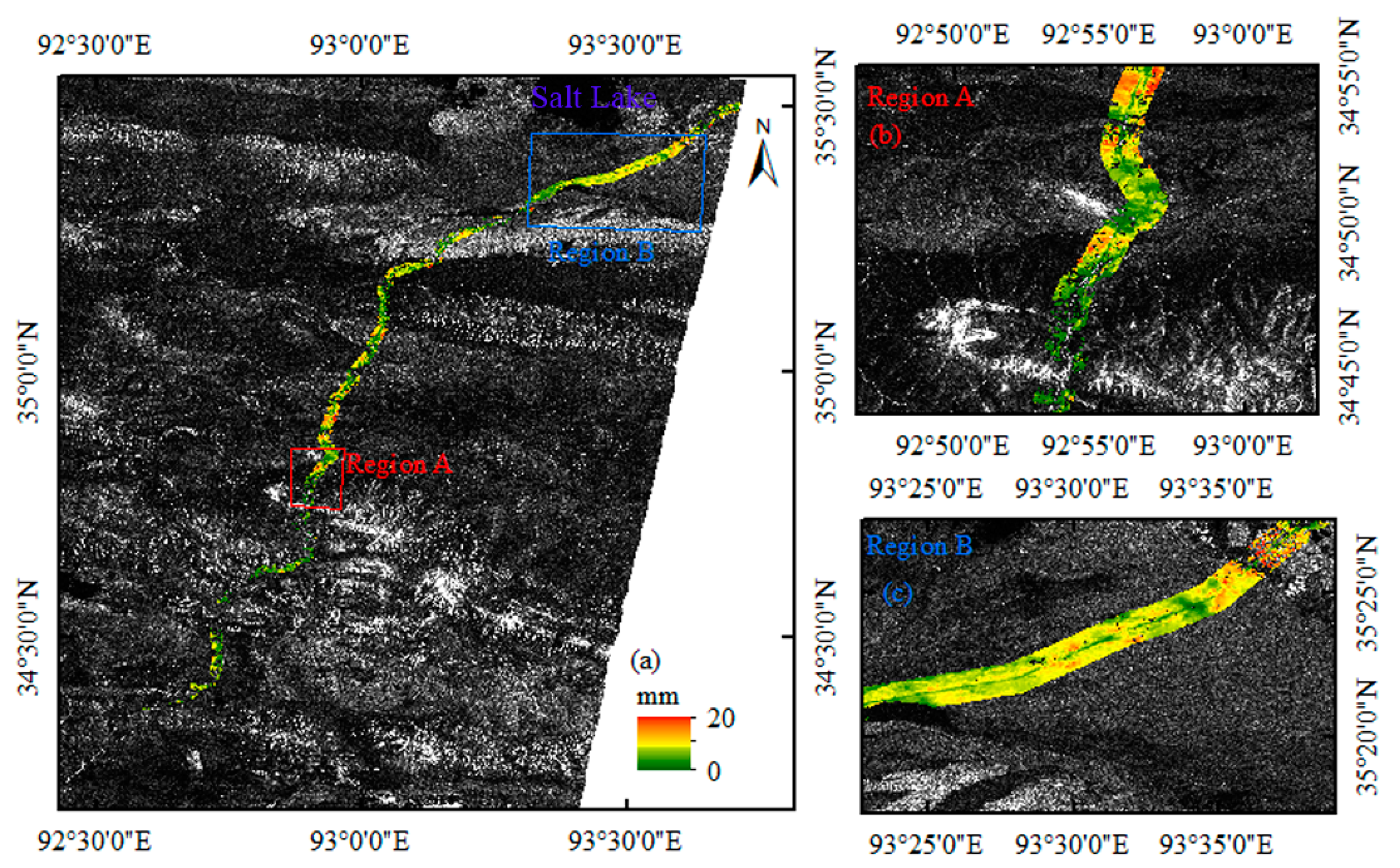
4.2. Deformation Time Series

The deformation time series of the study area is presented in Figure 7. It can be seen that the peak-to-peak seasonal displacements within the year from December 2017 to December 2018 reached 80 mm in some areas. Most of the areas had peak-to-peak seasonal displacement of nearly 40 mm (Figure 7, Figure 8 box of median value). Temporal deformation statistics (Figure 8a,b) showed that the surface deformation over the permafrost region was characterized by a periodicity cycle within the year, in which freeze-thaw induced alternating uplift and subsidence. Therefore, the surface subsided significantly from April to October and uplifted from October to March. Discontinuous surface subsidence or uplift were found in some time periods (Figure 8a,b). For example, deformation abnormality occurred on 31 August 2018 both on the alpine meadow and in the alpine desert region. It can also be seen from Figure 8a,b that rapid uplift and subsidence occurred in the first one to two months of a deformation transition period and then slowed down in the following months. The reason was that the thaw of the active layer was the greatest early in the summer, slowing considerably in August and September. Active layers thaw from ground surface to bottom depended on the heat transmission, the melting rate decreased with the deepening of the ALT, and correspondingly, the thaw settled down. For the temporal deformation of different soil characteristics, the alpine meadow had higher peak-to-peak seasonal displacement (box median value from −20 to 25 m) compared with alpine desert (box median value from −10 to 15 mm), which is consistent with the results in Figure 5. It can be seen from the box plot in Figure 8a that the alpine meadow had larger spatial variation (as indicated by box) within a specific period, while more outliers (red point) existed over the alpine desert. The reason is that the ALT and soil moisture vary more in vegetated regions than on bare lands, contributing to the large range of spatial variation, whereas due to the dry conditions and deep ALT over some areas of alpine desert, the displacement process did not correspond well to a seasonal model, which led to outliers.

Considering the spatial−temporal hydrological properties of permafrost, the soil moisture variation patterns of various types of land cover have been analyzed [53]. The results show that a positive temporal-spatial correlation was found between soil moisture and displacement in different land cover types. The surface/root zone soil moisture is a critical factor for discovering the origin of surface deformation variation. In this study, SMAP L4_SM surface and root zone daily soil moisture products were introduced to perform the analysis. SMAP L4_SM data provide quantitative estimates of surface and root zone soil moisture with −5 cm and 1 m depth over a 9 km grid [37], respectively. Although the 9 km-resolution grid is insufficient to characterize the spatial variation at a fine scale, it is a quite effective way to describe the temporal variation of deformation. As shown in Figure 8c,d, the surface and root zone soil moisture increased from June to October and was relatively stable in winter. It is obvious that the soil moisture storage in this year was higher than the previous year due to abundant rainfall (Figure 8c,d). The surface soil moisture in summer strongly varies because rainfall and evapotranspiration/infiltration occurred alternately, while the root zone soil moisture increased steadily due to the continuous melting process of ALT and surface soil moisture permeation in summer. According to Figure 8c,d, large surface soil moisture variation was found from April 1 to June 9, whereas the root zone soil moisture was still low, which means that the soil moisture variation in the early stage was mainly caused by soil thawing, while subsidence occurred in this period (Figure 8). The intrinsic difference in soil moisture content between different soil types affected the deformation rate (Figure 5). To quantitatively evaluate the influence of soil moisture on settlement deformation, the correlation analysis between relative deformation reference to November 28, 2017 and root zone soil moisture during thawing season (from 9 April 2018 to October 6, 2018) were performed. The correlation coefficient in alpine desert and alpine meadow were 0.45 and 0.81, respectively. Same as [53] positive temporal-spatial correlation was found in this study(Figure 9). As seen from Figure 9, the deformation in alpine meadow region is more susceptible to soil moisture than that of alpine desert.

The climatic conditions represent a key factor influencing the seasonal variations of the deformation. The interseason uplift and subsidence were mainly caused by variations of air and soil temperatures. Time-series verification statistics with three-day intervals were performed. As shown in Figure 10, the soil surface melting period ranged from 1 April to 7 October, which was consistent with the settlement period of the study area (Figure 8a,b). It should be noted that temperature oscillation existed in the beginning and ending periods, and recurrent subsidence and uplift were found in 3 May 2018–27 May 2018(Figure 7 and Figure 8a,b). However, deformation oscillation during the thawing period also existed, because in reality, seasonal deformation is affected by many other factors, such as precipitation [45].

5. Discussion

5.1. Comparison with Other Surface Displacement Studies in Permafrost

There are a lot of studies focus on permafrost thaw subsidence and freezing uplift in the QTP using sinusoidal models. To effectively validate this work, we compared our study with other researches in QTP permafrost regions using sinusoidal models (

Table 1. Parameters of previous studies on Qinghai–Tibetan Plateau (QTP) using sinusoidal models.

Authors	Study Area	SAR Dataset	Observation Period	Seasonal Oscillations Amplitude (mm)
Daout et.al.2017 [3]	Northwestern QTP	Envisat ASAR	2003–2011	2.5–12
Jia et.al. 2017 [17]	Same as this study	ALOS PALSAR	2007–2009	0–20
Li et.al. 2015 [46]	Southern QTP	Envisat ASAR	2007–2011	0.5–28
This study	South of Qinghai province	Sentinel-1	2017.11–2018.12	0–30

). Daout et al. [3] observed seasonal amplitude of 2.5–12 mm from 2003 to 2011. Li et al. [45] reported seasonal oscillations ranging from 0.5 to 28 mm during 2007–2011. Jia et al. [17] showed the peak-to peak amplitudes of seasonal oscillations of an area along QTR ranging from 0 to 2 cm during 2007–2009. Similar season oscillations and deformation trends were acquired in our study, but they still had some differences. The reason is that those case studies were conducted at different study areas and time periods. In this study, the time-series analysis was conducted in the most recent period, which allowed us to monitor the most recent condition of deformation. In addition, historical studies mainly focus on the interannual season deformation with a long temporal baseline, which lacked detailed features of seasonal deformation. We made up for this deficiency through 12-day interval images, so more detailed temporal displacement was acquired.

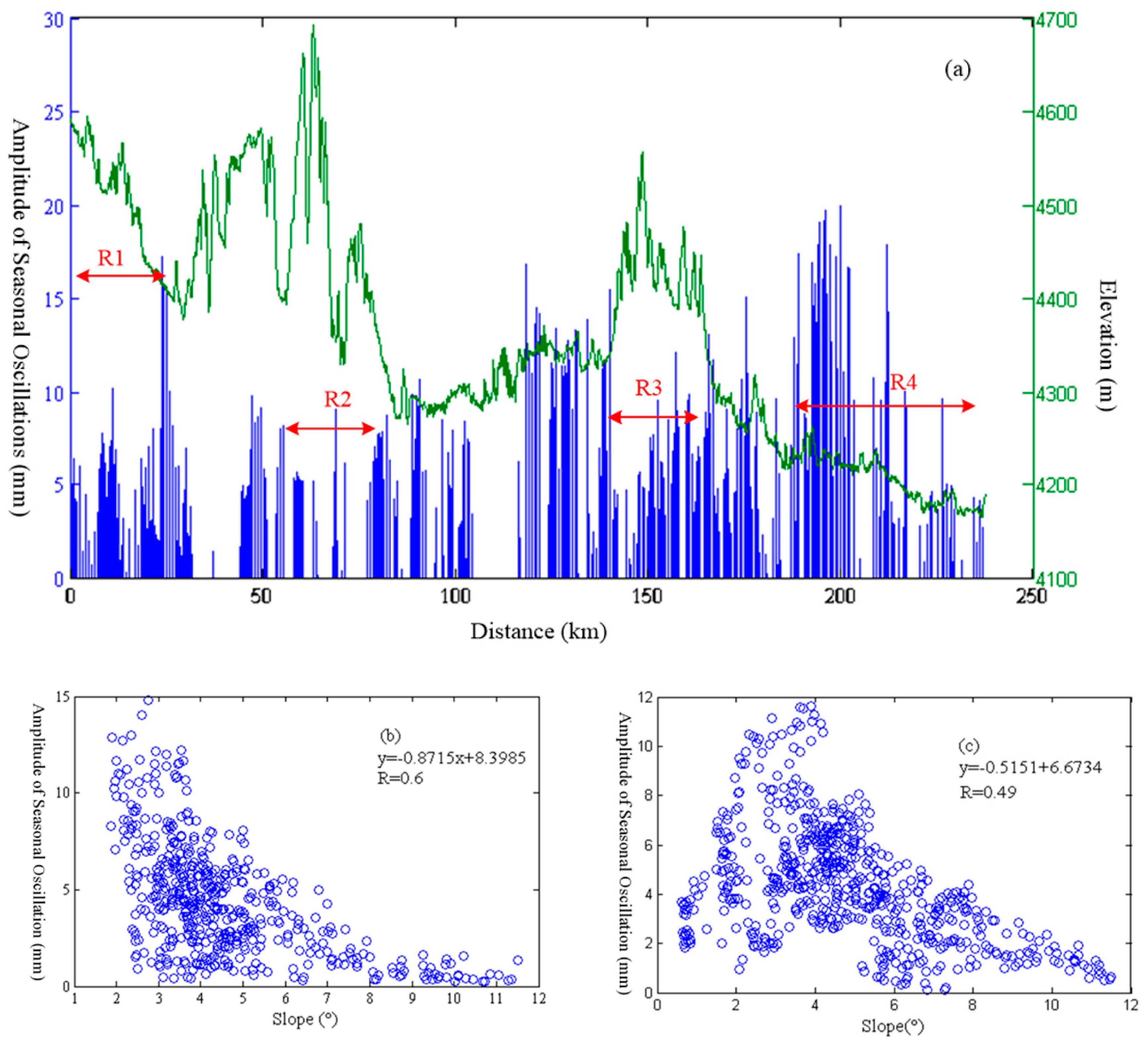
5.2. Seasonal Amplitude Dynamic Response of Topographical Factor

The amplitude of the seasonal movement was large over flat surfaces, while it decreased with the increase in altitude and slope. One reason is that in mountainous areas with high altitude are in less soil moisture storage and stable bedrock and the precipitation in these areas can only cause small variations to soil moisture. Moreover, considering the thermal properties of ALT, the seasonal deformation is positively related with ALT, whereas the ALT decreases with the increasing elevation due to the decrease in temperature [54]. The amplitude of the seasonal deformation is influenced by properties of the ground upper layer, further reflected in ALT [54]. These observations might be explained by a difference in the evapotranspiration, sensible heat flux, and surface flux [10,55]. The energy balance is controlled by the physical state of environment and surface properties, which is ultimately manifested in different amounts of deformation. A negative correlation was also found in [3].

5.3. Relation between Seasonal Amplitude and ALT

As mentioned above, the effect of deformation is controlled by the spatial and temporal variability of ALT. Previous studies have estimated ALT based on deformation results, which indicated that a close correspondence exists between seasonal deformation and ALT [17,36,45]. In those studies, quantitative relationships between the displacement of the permafrost surface and ALT have been developed. The relationship models are mainly controlled by multilayered groundwater content distribution and soil porosity. In this study, topography and geology responses were also discovered (Figure 8 and Figure 4). GPR is used to study the hydrological features of ice-content melting, and to detect the demarcation line between melting layers and ice-bearing layers under different types of land cover (Figure 5 and Figure 11). As shown in Figure 11a,b, ALT varies with vegetation type. The average melting depth in alpine meadow and alpine desert were 2.5 m and 3 m, respectively. Compared with the amplitude profiles of seasonal oscillation results shown in Figure 5 and Figure 11c,d, the difference of seasonal amplitude between two in-situ locations was obvious. The in situ ALT results explained the effect of surface and underground on displacement. It should be noted that the ALT was not only affected by vegetation and climatic factors but also by topography, lithology and hydrological conditions. We also found from the GPR measurements that the ALT showed significant spatial variations even for the same type of land cover.

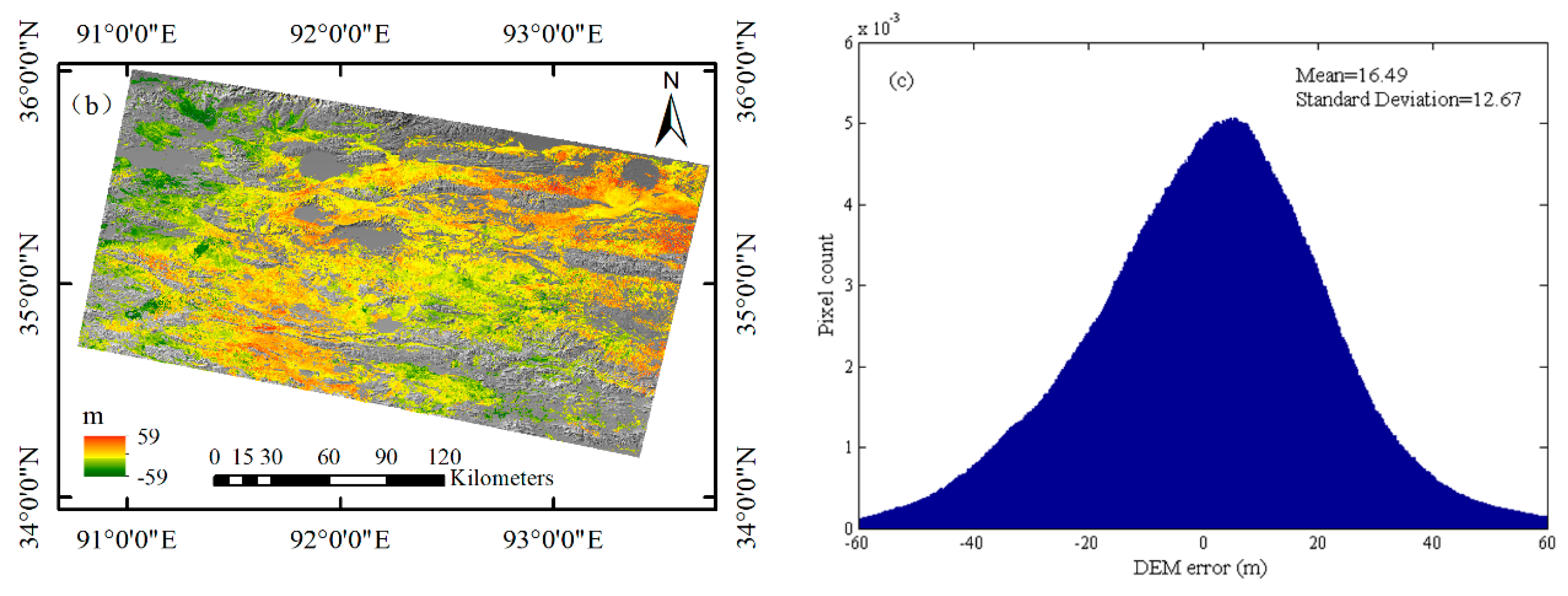
5.4. Time-Varying Error of Seasonal Displacement

According to the surface and root soil moisture variation result, variation can be used to explain the deformation caused by rainfall. Comparing Figure 8a,b and Figure 8c,d, it can be observed that the deformation oscillation (26 July–24 September) occurred in a period of large soil moisture variation. Rain storms in the thawing season in the area of the QTP can dramatically increase the soil moisture, causing a ground uplift signal in an interferogram, as well as discontinuous subsidence [9]. The daily surface soil moisture change is a key indicator for rainfall. Changing soil moisture conditions have been identified as a potential source of MT-InSAR errors.

Table 2. Cumulative displacements relative to first acquisition date, surface temperature and surface soil moisture in specific period over P1 (Figure 6).

Observation Date	Surface Temperature (°)	Surface Soil Moisture (m3/m−3)	Cumulative Displacement (mm)
3 May 2018	2.85	0.162	7.8
15 May 2018	4.85	0.154	−1.2
27 May 2018	0.15	0.131	2.1
19 August 2018	5.85	0.256	−7.3
31 August 2018	1.15	0.283	3.2
12 September 2018	1.15	0.25	0.5

showed the significant impact of surface moisture variation. Compared with 19 August 2018 and 12 September 2018, soil moisture on 31 August 2018 was larger, the cumulative displacement anomaly was observed on 31 August 2018. From 3 May 2018 to 27 May 2018, the effect of soil moisture variation was not shown, while the displacement anomaly could be explained by the surface temperature variation.

First, the climate anomalies during the study period that lead to deformation were not well described by the sinusoidal function seasonal model. On the other hand, from August to September, there was abundant rainfall in QTP. According to our in-situ soil moisture measurements from 27 August to 2 September, the soil water content in alpine meadow and alpine desert was very high, while the soil moisture change impacted the measured phase, which may correspond to the displacement error of about 10% of the radar wavelength on bare soil and lead to an error of 3 mm–3 cm [56]. In addition, the melting layer on the top of permafrost got drier and drier in summer, and the spurious drying-induced uplift observed in the DInSAR estimation may mask the actual surface subsidence [57].

In this study, the sinusoidal model–based NSBAS method is proved to be suitable for modeling of the ground surface deformation of the frozen soil. However, some discrepancies were identified, especially over mountainous areas, such as the DEM error, which could not be removed through the error modeling in this study. Moreover, as [17,45] mentioned, the freezing-thawing seasonal deformation is affected by many factors, such as precipitation, temperature, water content, heat flow, surface erosion, and tectonic movement, which may cause bias and deviation from the sinusoidal model.

6. Conclusions

In this paper, we applied sinusoidal model–based NSBAS using Sentinel-1 data acquired from 28 November 2017 to 29 December 2018 to monitor the freeze−thaw seasonal displacements over the selected permafrost region of QTP. Based on the results obtained, the following conclusions can be drawn.

First, the peak-to-peak amplitude of seasonal surface deformation in the study area ranged from 0 to 30 mm. The amplitude of the seasonal movement was influenced by terrain properties, being negatively correlated with elevation and slope, with larger amplitude of seasonal movement over flat surfaces compared with mountainous areas. Spatial variations of the amplitude in different ecosystems showed obvious differences, with the average amplitude of 15 mm in the alpine meadow and 7 mm in the alpine desert areas, respectively. Field investigation results of ALT based on GPR verified the spatial heterogeneity quantitatively. Along the QTR, strong spatial variability was also discovered.

In addition, the deformation of time series in one year was monitored with the peak-to-peak seasonal displacement of 40 mm. The freeze and thaw time nodes were 24 September and 9 April, respectively, which are consistent with the surface temperature trends. There were spatial variations and anomalies in the study area in a specific period.

The NSBAS method based on the seasonal model is an effective method for monitoring freeze-thaw seasonal displacement of the permafrost on a large scale. Sentinel-1 data with shorter revisit time can successfully characterize the seasonal deformation response of frozen soil to surface temperature, soil moisture, and other factors. The results show that Sentinel-1 data with high temporal resolution are an effective data source for monitoring short-term surface displacement, which is useful for monitoring permafrost-related seasonal deformation, thereby helping us to better understand the surface dynamics of QTP permafrost region.

References

1. Kang, S.; Xu, Y.; You, Q.; Flügel, W.A.; Pepin, N.; Yao, T. Review of climate and cryospheric change in the Tibetan Plateau. Environ. Res. Lett. 2010, 5, 8–16. [Google Scholar] [CrossRef]
2. Wang, L.; Marzahn, P.; Bernier, M.; Jacome, A.; Poulin, J.; Ludwig, R. Comparison of TerraSAR-X and ALOS PALSAR Differential Interferometry With Multisource DEMs for Monitoring Ground Displacement in a Discontinuous Permafrost Region. IEEE J. Sel. Top. Appl. Earth Obs. Remote Sens. 2017, 10, 4074–4093. [Google Scholar] [CrossRef]
3. Daout, S.; Doin, M.P.; Peltzer, G.; Socquet, A.; Lasserre, C. Large-scale InSAR monitoring of permafrost freeze-thaw cycles on the Tibetan Plateau. Geophys. Res. Lett. 2017, 44, 901–909. [Google Scholar] [CrossRef]
4. Short, N.; Brisco, B.; Couture, N.; Pollard, W.; Murnaghan, K.; Budkewitsch, P. A comparison of TerraSAR-X, RADARSAT-2 and ALOS-PALSAR interferometry for monitoring permafrost environments, case study from Herschel Island, Canada. Remote Sens. Environ. 2011, 115, 3491–3506. [Google Scholar] [CrossRef]
5. Rykhus, R.P.; Lu, Z. InSAR detects possible thaw settlement in the Alaskan Arctic Coastal Plain. Can. J. Remote Sens. 2008, 34, 100–112. [Google Scholar] [CrossRef]
6. Wolfe, S.A.; Short, N.H.; Morse, P.D.; Schwarz, S.H.; Stevens, C.W. Evaluation of RADARSAT-2 DInSAR Seasonal Surface Displacement in Discontinuous Permafrost Terrain, Yellowknife, Northwest Territories, Canada. Can. J. Remote Sens. 2014, 40, 406–422. [Google Scholar] [CrossRef]
7. Beck, I.; Ludwig, R.; Bernier, M.; Strozzi, T.; Boike, J. Vertical movements of frost mounds in subarctic permafrost regions analyzed using geodetic survey and satellite interferometry. Earth Surf. Dyn. 2015, 3, 409–421. [Google Scholar] [CrossRef]
8. Strozzi, T.; Wegmuller, U.; Werner, C.; Kos, A. TerraSAR-X interferometry for surface deformation monitoring on periglacial area. In Proceedings of the 2012 IEEE International Geoscience and Remote Sensing Symposium, Munich, Germany, 22–27 July 2012; pp. 5214–5217. [Google Scholar]
9. Liu, L.; Zhang, T.J.; Wahr, J. InSAR measurements of surface deformation over permafrost on the North Slope of Alaska. J. Geophys. Res. Earth Surf. 2010, 115. [Google Scholar] [CrossRef]
10. Antonova, S.; Sudhaus, H.; Strozzi, T.; Zwieback, S.; Kaab, A.; Heim, B.; Langer, M.; Bornemann, N.; Boike, J. Thaw Subsidence of a Yedoma Landscape in Northern Siberia, Measured In Situ and Estimated from TerraSAR-X Interferometry. Remote Sens. 2018, 10, 494. [Google Scholar] [CrossRef]
11. Chen, F.L.; Lin, H.; Zhou, W.; Hong, T.H.; Wang, G. Surface deformation detected by ALOS PALSAR small baseline SAR interferometry over permafrost environment of Beiluhe section, Tibet Plateau, China. Remote Sens. Environ. 2013, 138, 10–18. [Google Scholar] [CrossRef]
12. Zhao, R.; Li, Z.W.; Feng, G.C.; Wang, Q.J.; Hu, J. Monitoring surface deformation over permafrost with an improved SBAS-InSAR algorithm: With emphasis on climatic factors modeling. Remote Sens. Environ. 2016, 184, 276–287. [Google Scholar] [CrossRef]
13. Li, Y.; Zhang, J.; Li, Z.; Luo, Y.; Jiang, W.; Tian, Y. Measurement of subsidence in the Yangbajing geothermal fields, Tibet, from TerraSAR-X InSAR time series analysis. Int. J. Digit. Earth 2016, 9, 697–709. [Google Scholar] [CrossRef]
14. Wang, C.; Zhang, Z.J.; Zhang, H.; Wu, Q.B.; Zhang, B.; Tang, Y.X. Seasonal deformation features on Qinghai-Tibet railway observed using time-series InSAR technique with high-resolution TerraSAR-X images. Remote Sens. Lett. 2017, 8, 1–10. [Google Scholar] [CrossRef]
15. Dai, K.R.; Liu, G.X.; Li, Z.H.; Ma, D.Y.; Wang, X.W.; Zhang, B.; Tang, J.; Li, G.Y. Monitoring Highway Stability in Permafrost Regions with X-band Temporary Scatterers Stacking InSAR. Sensors 2018, 18, 1876. [Google Scholar] [CrossRef]
16. Wang, C.; Zhang, H.; Zhang, B.; Tang, Y.; Zhang, Z.; Liu, M.; Zhao, L. New mode TerraSAR-X interferometry for railway monitoring in the permafrost region of the Tibet Plateau. In Proceedings of the 2015 IEEE International Geoscience and Remote Sensing Symposium (IGARSS), Milan, Italy, 26–31 July 2015; pp. 1634–1637. [Google Scholar]
17. Jia, Y.Y.; Kim, J.W.; Shum, C.K.; Lu, Z.; Ding, X.L.; Zhang, L.; Erkan, K.; Kuo, C.Y.; Shang, K.; Tseng, K.H.; et al. Characterization of Active Layer Thickening Rate over the Northern Qinghai-Tibetan Plateau Permafrost Region Using ALOS Interferometric Synthetic Aperture Radar Data, 2007–2009. Remote Sens. 2017, 9, 84. [Google Scholar] [CrossRef]
18. Chang, L.; Hanssen, R.F. Detection of permafrost sensitivity of the Qinghai-Tibet railway using satellite radar interferometry. Int. J. Remote Sens. 2015, 36, 691–700. [Google Scholar] [CrossRef]
19. Hooper, A.; Bekaert, D.; Spaans, K.; Arıkan, M. Recent advances in SAR interferometry time series analysis for measuring crustal deformation. Tectonophysics 2012, 514, 1–13. [Google Scholar] [CrossRef]
20. Zhang, Z.J.; Wang, C.; Zhang, H.; Tang, Y.X.; Liu, X.G. Analysis of Permafrost Region Coherence Variation in the Qinghai-Tibet Plateau with a High-Resolution TerraSAR-X Image. Remote Sens. 2018, 10, 298. [Google Scholar] [CrossRef]
21. Berardino, P.; Fornaro, G.; Lanari, R.; Sansosti, E. A new algorithm for surface deformation monitoring based on small baseline differential SAR interferograms. IEEE Trans. Geosci. Remote Sens. 2002, 40, 2375–2383. [Google Scholar] [CrossRef]
22. Devanthery, N.; Crosetto, M.; Monserrat, O.; Cuevas-Gonzalez, M.; Crippa, B. An Approach to Persistent Scatterer Interferometry. Remote Sens. 2014, 6, 6662–6679. [Google Scholar] [CrossRef]
23. Werner, C.; Wegmuller, U.; Strozzi, T.; Wiesmann, A. Interferometric point target analysis for deformation mapping. In Proceedings of the 2003 IEEE International Geoscience and Remote Sensing Symposium, Toulouse, France, 21–25 July 2003; pp. 4362–4364. [Google Scholar]
24. Ferretti, A.; Prati, C.; Rocca, F. Permanent scatterers in SAR interferometry. IEEE Trans. Geosci. Remote Sens. 2001, 39, 8–20. [Google Scholar] [CrossRef]
25. Zhang, L.; Ding, X.; Lu, Z. Modeling PSInSAR Time Series Without Phase Unwrapping. IEEE Trans. Geosci. Remote Sens. 2010, 49, 547–556. [Google Scholar] [CrossRef]
26. Solari, L.; Barra, A.; Herrera, G.; Bianchini, S.; Monserrat, O.; Bejar-Pizarro, M.; Crosetto, M.; Sarro, R.; Moretti, S. Fast detection of ground motions on vulnerable elements using Sentinel-1 InSAR data. Geomat. Nat. Hazards Risk 2018, 9, 152–174. [Google Scholar] [CrossRef]
27. Barra, A.; Solari, L.; Bejar-Pizarro, M.; Monserrat, O.; Bianchini, S.; Herrera, G.; Crosetto, M.; Sarro, R.; Gonzalez-Alonso, E.; Mateos, R.M.; et al. A Methodology to Detect and Update Active Deformation Areas Based on Sentinel-1 SAR Images. Remote Sens. 2017, 9, 1002. [Google Scholar] [CrossRef]
28. Xie, C.; Li, Z.; Xu, J.; Li, X.W. Analysis of deformation over permafrost regions of Qinghai-Tibet plateau based on permanent scatterers. Int. J. Remote Sens. 2010, 31, 1995–2008. [Google Scholar] [CrossRef]
29. Hooper, A.; Zebker, H.; Segall, P.; Kampes, B. A new method for measuring deformation on volcanoes and other natural terrains using InSAR persistent scatterers. Geophys. Res. Lett. 2004, 31. [Google Scholar] [CrossRef]
30. Chen, J.; Liu, L.; Zhang, T.J.; Cao, B.; Lin, H. Using Persistent Scatterer Interferometry to Map and Quantify Permafrost Thaw Subsidence: A Case Study of Eboling Mountain on the Qinghai-Tibet Plateau. J. Geophys. Res. Earth Surf. 2018, 123, 2663–2676. [Google Scholar] [CrossRef]
31. Zhang, Z.; Wang, C.; Wang, M.; Wang, Z.; Zhang, H. Surface deformation monitoring in Zhengzhou city from 2014 to 2016 using time-series insar. Remote Sens. 2018, 10, 1731. [Google Scholar] [CrossRef]
32. Ferretti, A.; Fumagalli, A.; Novali, F.; Prati, C.; Rocca, F.; Rucci, A. A new algorithm for processing interferometric data-stacks: SqueeSAR. IEEE Trans. Geosci. Remote Sens. 2011, 49, 3460–3470. [Google Scholar] [CrossRef]
33. Perissin, D.; Wang, T. Repeat-Pass SAR Interferometry With Partially Coherent Targets. IEEE Trans. Geosci. Remote Sens. 2012, 50, 271–280. [Google Scholar] [CrossRef]
34. Zhang, L.; Zhong, L.U.; Ding, X.; Jung, H.S.; Feng, G.; Lee, C.-W. Mapping ground surface deformation using temporarily coherent point SAR interferometry: Application to Los Angeles Basin. Remote Sens. Environ. 2012, 117, 429–439. [Google Scholar] [CrossRef]
35. Dong, D.; Fang, P.; Bock, Y.; Cheng, M.K.; Miyazaki, S. Anatomy of apparent seasonal variations from GPS-derived site position time series. J. Geophys. Res. Solid Earth 2002, 107. [Google Scholar] [CrossRef]
36. Wang, C.; Zhang, Z.; Zhang, H.; Zhang, B.; Tang, Y.; Wu, Q. Active Layer Thickness Retrieval of Qinghai–Tibet Permafrost Using the TerraSAR-X InSAR Technique. IEEE J. Sel. Top. Appl. Earth Obs. Remote Sens. 2018, 11, 4403–4413. [Google Scholar] [CrossRef]
37. Zhang, X.; Zhang, T.; Ping, Z.; Yun, S.; Shan, G. Validation Analysis of SMAP and AMSR2 Soil Moisture Products over the United States Using Ground-Based Measurements. Remote Sens. 2017, 9, 104. [Google Scholar] [CrossRef]
38. Gusmeroli, A.; Liu, L.; Schaefer, K.; Zhang, T.; Schaefer, T.; Grosse, G. Active Layer Stratigraphy and Organic Layer Thickness at a Thermokarst Site in Arctic Alaska Identified Using Ground Penetrating Radar. Arct. Antarct. Alp. Res. 2015, 47, 195–202. [Google Scholar] [CrossRef]
39. Xie, F.; Wang, C.C. The Application of LTD-2100 GPR (Ground Penetrating Radar) in Inspection of Concrete Structures. Adv. Mater. Res. 2012, 424–425, 1282–1286. [Google Scholar] [CrossRef]
40. Jarvis, A.; Reuter, H.I.; Nelson, A.; Guevara, E. Hole-filled SRTM for the globe Version 4. 2008. Available online: https://www.researchgate.net/publication/225091464_Hole-filled_SRTM_for_the_globe_version_3_from_the_CGIAR-CSI_SRTM_90m_database (accessed on 30 October 2018).
41. Costantini, M. A novel phase unwrapping method based on network programming. IEEE Trans. Geosci. Remote Sens. 1998, 36, 813–821. [Google Scholar] [CrossRef]
42. Sandwell, D.; Mellors, R.; Tong, X.; Wei, M.; Wessel, P. GMTSAR: An InSAR Processing System Based on Generic Mapping Tools. Available online: https://escholarship.org/uc/item/8zq2c02m (accessed on 30 October 2018).
43. Jolivet, R.; Grandin, R.; Lasserre, C.; Doin, M.P.; Peltzer, G. Systematic InSAR atmospheric phase delay corrections from global meteorological reanalysis data. Geophys. Res. Lett. 2011, 38, 351–365. [Google Scholar] [CrossRef]
44. Biggs, J.; Wright, T.; Lu, Z.; Parsons, B. Multi-interferogram method for measuring interseismic deformation: Denali Fault, Alaska. Geophys. J. Int. 2007, 170, 1165–1179. [Google Scholar] [CrossRef]
45. Li, Z.; Zhao, R.; Hu, J.; Wen, L.; Feng, G.; Zhang, Z.; Wang, Q. InSAR analysis of surface deformation over permafrost to estimate active layer thickness based on one-dimensional heat transfer model of soils. Sci. Rep. 2015, 5, 15542. [Google Scholar] [CrossRef] [PubMed]
46. Hetland, E.; Musé, P.; Simons, M.; Lin, Y.; Agram, P.; DiCaprio, C. Multiscale InSAR time series (MInTS) analysis of surface deformation. J. Geophys. Res. Solid Earth 2012, 117. [Google Scholar] [CrossRef]
47. López-Quiroz, P.; Doin, M.P.; Tupin, F.; Briole, P.; Nicolas, J.M. Time series analysis of Mexico City subsidence constrained by radar interferometry. J. Appl. Geophys. 2009, 69, 1–15. [Google Scholar] [CrossRef]
48. Doin, M.-P.; Lodge, F.; Guillaso, S.; Jolivet, R.; Lasserre, C.; Ducret, G.; Grandin, R.; Pathier, E.; Pinel, V. Presentation of the Small Baseline NSBAS Processing Chain on a Case Example: The Etna Deformation Monitoring from 2003 to 2010 Using Envisat Data. Available online: https://earth.esa.int/documents/10174/1573056/Presentation_small_baseline_NSBAS_Etna_deformation_Envisat.pdf (accessed on 30 October 2018).
49. Doin, M.P.; Twardzik, C.; Ducret, G.; Lasserre, C.; Guillaso, S.; Sun, J. InSAR measurement of the deformation around Siling Co Lake: Inferences on the lower crust viscosity in central Tibet. J. Geophys. Res. Solid Earth 2015, 120, 5290–5310. [Google Scholar] [CrossRef]
50. Agram, P.S.; Jolivet, R.; Riel, B.; Lin, Y.N.; Simons, M.; Hetland, E.; Doin, M.P.; Lasserre, C. New Radar Interferometric Time Series Analysis Toolbox Released. EOS Trans. Am. Geophys. Union 2013, 94, 69–70. [Google Scholar] [CrossRef]
51. Agram, P.; Jolivet, R.; Simons, M.; Riel, B. GIAnT-Generic InSAR Analysis Toolbox. Available online: ftp://ftp.gps.caltech.edu/pub/piyush/AGU_giant_high.pdf (accessed on 30 October 2018).
52. Jiang, X.; Li, C.; Sun, J. A modified K-means clustering for mining of multimedia databases based on dimensionality reduction and similarity measures. Clust. Comput. 2017, 21, 797–804. [Google Scholar] [CrossRef]
53. Wang, C.; Zhang, H.; Wu, Q.; Zhang, Z.; Xie, L. Monitoring permafrost soil moisture with multi-temporal TERRASAR-X data in Northern Tibet. In Proceedings of the 2016 IEEE International Geoscience and Remote Sensing Symposium (IGARSS), Beijing China, 10–15 July 2016; pp. 3039–3042. [Google Scholar]
54. Riseborough, D.; Shiklomanov, N.; Etzelmuller, B.; Gruber, S.; Marchenko, S. Recent advances in permafrost modelling. Permafr. Periglac. Process. 2008, 19, 137–156. [Google Scholar] [CrossRef]
55. Langer, M.; Westermann, S.; Muster, S.; Piel, K.; Boike, J. The surface energy balance of a polygonal tundra site in northern Siberia - Part 1: Spring to fall. Cryosphere 2011, 5, 151–171. [Google Scholar] [CrossRef]
56. Zwieback, S.; Hensley, S.; Hajnsek, I. Soil Moisture Estimation Using Differential Radar Interferometry: Toward Separating Soil Moisture and Displacements. IEEE Trans. Geosci. Remote Sens. 2017, 55, 5069–5084. [Google Scholar] [CrossRef]
57. Short, N.; LeBlanc, A.-M.; Sladen, W.; Oldenborger, G.; Mathon-Dufour, V.; Brisco, B. RADARSAT-2 D-InSAR for ground displacement in permafrost terrain, validation from Iqaluit Airport, Baffin Island, Canada. Remote Sens. Environ. 2014, 141, 40–51. [Google Scholar] [CrossRef]
Figure 1. (a) Google Earth image of study area. (b) Shuttle radar topography mission (SRTM) digital elevation model (DEM) map of study area. (c) Sentinel-1 amplitude image of study area and location of Qinghai–Tibetan Plateau (QTR). (d) TerraSAR-X amplitude image in the blue box of (c).
Remotesensing 11 01000 g001
Figure 2. The flow chart of multitemporal interferometric synthetic aperture radar (MT-InSAR) applied in this study.
Remotesensing 11 01000 g002
Figure 3. (a) The amplitude of seasonal oscillation in the study area. (b) DEM error in the study area. (c) Frequency distribution histogram of DEM error.
Remotesensing 11 01000 g003aRemotesensing 11 01000 g003b
Figure 4. (a) Profiles of amplitude of seasonal deformation (blue) and elevation (green). (b) Correlation between slope and seasonal amplitude for profile zone B1−B2. (c) Correlation between slope and seasonal amplitude for profile zone C1−C2.
Remotesensing 11 01000 g004
Figure 5. The amplitude of seasonal oscillation under different land covers. (a) The amplitude map of high-resolution TerraSAR-X image (11 December 2015); (b) the classification result of TerraSAR-X image. (c) the amplitude of seasonal oscillations along profile A−B.
Remotesensing 11 01000 g005
Figure 6. (a) Amplitude variations along QTR using a 1 km buffer. (b) and (c) Zoomed-in images over region A and Region B from (a), respectively.
Remotesensing 11 01000 g006
Figure 7. Maps showing the deformation time series in the study area, relative to the first acquisition on 28 November 2017.
Remotesensing 11 01000 g007
Figure 8. (a) Deformation time series statistics results over alpine meadow (P1); (b) Deformation time series statistics results over alpine desert (P2) (the positions of P1 and P2 are shown in Figure 5a). Time-series surface soil moisture (c) and root zone soil moisture (d) for soil moisture active/passive (SMAP) L4 data over the study area( Presented are the median (red line), the first quantile Q1 and third quantile Q3 (as indicated by box), and the Q1 − 1.5(Q3 − Q1) and Q3 + 1.5(Q3 − Q1) value(whiskers) and outliers (red point)).
Remotesensing 11 01000 g008
Figure 9. Time series correlation analysis between root zone soil moisture and relative deformation in thawing season from 9 April 2018 to 6 October, 2018.
Remotesensing 11 01000 g009
Figure 10. Time series of surface temperature of SMAP L4 data in the study area.
Remotesensing 11 01000 g010
Figure 11. (a) In situ active layer thickness (ALT) profile of Alpine meadow based on ground-penetrating radar (GPR) (August 28, 2018). (b) In situ ALT profile of Alpine desert based on GPR (August 28, 2018). (c) The amplitude of seasonal oscillation surrounding (a). (d) The amplitude of seasonal oscillation surrounding (b).
Remotesensing 11 01000 g011