Abstract
Variability of sea level in the North and Baltic Seas, enforced by weather patterns, affects the intensity of water exchange between these seas. Transfer of salty water from the North Sea is very important for the hydrography of the Baltic Sea. The volume of inflowing salty water can occasionally increase remarkably. Such incidents, called the Major Baltic Inflows (MBIs), are unpredictable, of relatively short duration, and difficult to observe using in situ data. We have shown that remote sensing altimetry can be used as a complementary source of information about the MBI events. The advantage of using such data is that large-scale spatial information about SLA is available with daily resolution. We have described changes in SLA during several MBI events observed in 1993–2017. The net volume of water transported into the Baltic Sea varied between the events due to differences in atmospheric forcing. Based on SLA data, the largest inflow of water happened during the 2014 MBI. This is in agreement with previously published results, based on in situ data.
1. Introduction
The Baltic Sea (BS) is an inland brackish sea situated in northern Europe (Figure 1). The average depth of this sea is about 56 m. The physical properties of seawater reflect the fact that a substantial amount of freshwater (about 480 km3) is added annually to the Baltic Sea by rivers and atmospheric input. River runoff is about one order of magnitude larger than the net input from precipitation and evaporation [1]. Considerable inflow of freshwater decreases seawater salinity and maintains a permanent two-layer salinity structure in the Baltic Sea. A persistent halocline is observed and an estuarine-like water exchange with the North Sea takes place. Water residence time in the Baltic Sea is about 30 years. Low salinity waters coming out of the Baltic Sea have a significant impact on the hydrography of the North and Norwegian Seas [1]. In contrast, most of the time, there is only a weak inflow of dense and salty water into the Baltic Sea from the North Sea (through the Danish Straits, Skagerrak, and Kattegat). The intensity of this inflow can occasionally, at irregular intervals of time, increase impressively. Such incidents, called the Major Baltic Inflows (MBI), depend on weather patterns, which control the sea-level difference between the Baltic and the North Seas [2]. Major Baltic Inflows are difficult to predict, but have a fundamental influence on the conditions in the Baltic Sea [1]. For example, organisms living in the deep waters of the Baltic Sea strongly depend on inflows of highly saline and oxygenated water from the North Sea. These events are the only mechanism by which the central Baltic deep water is being renewed.
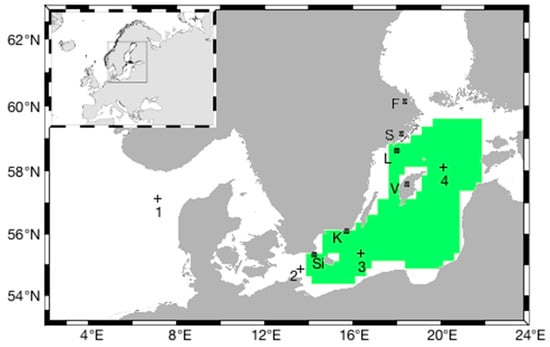
Figure 1.
Map of the Baltic Sea. Green color denotes the area of the Baltic Sea Proper used to estimate the mean SLA. Positions of selected pixels (1–4) used in the discussion of Sea Level Anomalies are indicated by crosses, while coastal tide gauge stations are indicated by black dots (Si = Simrishamn. K = Kungsholmsfort. V = Visby. L= Landsort Norra. S = Stockholm. F = Forsmark). The insert in the upper left corner shows the location of the Baltic Sea in Europe.
Thus, the overall process of exchange of water between the Baltic Sea and the North Sea includes three main components. The first component is almost continuous outflow of the low-salinity Baltic Sea water into the North Sea. This outflow is sustained by the excess input of freshwater from rivers and net precipitation. The outflow is directed into the Kattegat. The second component is associated with the baroclinic pressure gradient across the Danish Straits due to the salinity difference between the Kattegat (34) and the Arkona Basin (8). This pressure gradient stimulates the intermittent baroclinic inflows of saline water into the Baltic Sea [3,4,5,6]. Lastly, the barotropic inflows are the third component. They occur when the sea level difference between the Kattegat and the Baltic Sea becomes sufficiently large to enforce an additional inflow of salty waters into the western Baltic Sea [2,7,8,9]. When these sporadic inflows exceed 100 km3 of water, they are classified as the MBIs.
It was estimated [2] that 96 MBIs happened in the time interval between 1897 and 1997 (data were not collected during the two world wars). The MBIs took place between the end of August and the end of April, with 90% of the events occurring between October and February. In addition, the interannual variability was significant. Before the mid-1970s, the MBIs were more frequent, and later their frequency and intensity decreased. As a result, the deep waters in the central Baltic Sea experienced a prolonged period of stagnation [10,11]. In January 1993 and 2003, two isolated MBIs were documented [12,13], but they were not sufficient to substantially renew deep waters. Therefore, stagnant conditions in the BS continued until 2014, when a strong MBI was observed and followed by additional MBIs in 2015 and 2016 [14,15,16].
Observations indicated that each of the MBIs consists of a similar sequence of circumstances [9]. It is believed that a prerequisite for the barotropic MBI is the preliminary phase with easterly winds lasting on a time scale of the Baltic barotropic relaxation time (about 10 days) or longer. Easterly winds move surface waters out of the Baltic Sea. Consequently, the sea level in the central Baltic Sea can descend by about 0.5 m [11]. Often, this situation is associated with a stable high-pressure meteorological system over Scandinavia. This preliminary MBI phase is followed by strong and prolonged (at least one week) westerly winds, which force salty waters from the North Sea into the Baltic [2,11]. This is a proper inflow phase. During the MBI, the volume of the inflowing waters and the amount of transported salt is large (Table 1). After passing the shallow Danish Straits (Little Belt, Great Belt and Sound), the salty waters propagate as dense bottom currents toward the central Baltic Sea. They arrive to the central Baltic about 3 to 6 months after the start of the inflow event [17,18,19]. Time delay depends on the amount and density of the new inflowing water compared to the old water deposited in the Bornholm Basin after the previous inflow. With time, the new dense water masses are modified in the Western Baltic Sea by the entrainment of brackish waters [20,21]. While minor barotropic inflow events are observed several times a year at intermediate water depths [3], the MBIs that are strong enough to replace the bottom water in the central Baltic Sea occur on average only once every 3 to 10 years [11]. The irregular and infrequent occurrence as well as the short duration of the MBIs (about two to three weeks) presents a challenge to in situ observations of these events.

Table 1.
Five strongest Major Baltic Inflows since 1897 [1].
Recently, permanent moorings have been established with a goal of continuous hydrographic measurements for better monitoring the occurrence of the MBIs [11]. Another possible means to improve the understanding of the MBIs is through satellite observations. The main goal of this paper is to examine the satellite altimetry data and to explore if the MBIs can be observed using satellite observations. In comparison to the previous studies listed above, our analysis is based on open sea satellite-derived sea level data that are not affected by coasts and have better spatial resolution than the tide gauge data. Unfortunately, satellite altimetry data available for our analysis are considerably shorter (~ 25 years) than the historical tide gauge data. For example, in Stockholm, data were collected since 1774 [22]. Therefore, we will discuss only more recent events. Our research should be of interest to regional physical oceanographers interested in better understanding conditions favoring the occurrence of MBI events.
2. Materials and Methods
This article is based on analysis of satellite and other oceanographic data sets obtained from different sources. In each case, we have used 25-year-long (1993–2017) time series.
2.1. Satellite Sea Level Anomaly Data
To describe the variability of the sea level, we have used sea level anomalies (SLA) extracted from the delayed time (DT) multi-mission global gridded data product distributed by the Copernicus Marine and Environment Monitoring Service (CMEMS) (http://marine.copernicus.eu). The SLA data are referenced to the 20-year (1993–2012) mean sea surface height. Data were corrected for instrumental noise, orbit determination error, atmospheric attenuation (wet and dry tropospheric and ionospheric influences), sea state bias, and tidal influence [23]. The tidal aliasing correction was based on tidal models that assimilate altimetry data [24]. The SLA data were interpolated on a 0.25° × 0.25° spatial grid with one-day temporal resolution, using computing methods based on objective analysis. Details about data processing methods are explained at www.aviso.oceanobs.com. The error in the SLA data is about 1 to 2 cm. The results from a comprehensive validation of gridded satellite altimetry data product are available at hwww.aviso.altimetry.fr/en/data/products/ocean-indicators-products/mean-sea-level/validation.html. Altimetry data have been used before to discuss sea level trends and variability in the Baltic Sea [25,26,27,28,29,30]. The data set used in the present paper covers the time period from 1 January 1993 to 31 December 2017 (25 years). In order to discuss SLA changes in time, we have selected few pixels (Figure 1) where we have extracted time series data. Pixels 2–4 are located within the Baltic Proper. For comparison, we have also extracted time series data for one location in the North Sea, near the Skagerrak (pixel 1). The geographical coordinates corresponding to each time series record are listed in Table 2. The exact positions of these points are not crucial for our discussion. We merely wanted to show some examples of time series data. In addition, we have averaged SLA data over the area of the Baltic Proper (Figure 1) in order to estimate the change of the volume of water in the Baltic Sea due to the MBIs. The extent of this region has been limited to the Baltic Proper, in order to avoid contamination of the sea level time series by sea ice in the winter time.
Table 2.
Geographical positions of stations indicated in Figure 1.
2.2. ERA Interim Data
Wind and sea level pressure data have been used to characterize the meteorological conditions. Data were obtained from the European Center for Medium-Range Weather Forecasts (ECMWF) through the ERA-Interim reanalysis service (http://apps.ecmwf.int/datasets/data/interim-full-daily/). In the reanalysis, satellite data, in situ observations, and models are combined in an optimal way to derive consistent estimates of various atmospheric and oceanographic quantities. The ERA-Interim reanalysis has been carried out with a sequential data assimilation scheme, advancing forward in time. In each cycle, all available observations from in situ and satellite observations are combined with a forecast model to estimate the evolving state of the global atmosphere and its underlying surface. Daily data with 0.125° spatial resolution are used in the present work. Wind speed and direction at 10 m above sea level is given in a meteorological convention. This means that the U component is positive for a west to east wind, while the V component is positive for south to north wind. For a more detailed description of the ERA-Interim reanalysis data, the reader is referred to Reference [31] and http://www.ecmwf.int/research/era.
2.3. Tide Gauge Data
For a comparison with satellite data, we have used data from six coastal stations from the Baltic Sea (listed in Table 2 and indicated in Figure 1). We have used hourly tide gauge records provided by the SMHI (http://opendata-catalog.smhi.se/explore). Local tide gauges measure the sea level at a single location relative to local land surface, which is a measurement referred to as relative sea level (RSL). However, all sea level stations used in this paper were referenced to the Swedish national reference datum RH2000, also known as the Baltic Sea Chart Datum 2000 (BSCD2000). Downloaded, delayed mode data have been already screened and quality controlled at SMHI using the procedures described by GLOSS (The Global Sea Level Observing System), IODE (International Oceanographic Data and Information Exchange program of the Intergovernmental Oceanographic Commission at UNESCO), and CMEMS (The Copernicus Marine Environment Monitoring Service). It has to be noted that local sea levels at coastal stations are influenced by the variability of coastal currents and weather patterns, which can lead to significant storm surges in the Baltic Sea. These effects depend mostly on the local coastal topography, atmospheric pressure, wind speed, and direction. The SLA data used in this paper represent open sea conditions and are not influenced by coastal effects. Therefore, we would not expect a perfect agreement between the variability of SLA and coastal tide gauge data.
2.4. Runoff Data
On average, the mean river discharge in the Baltic Sea is about 10 times larger than the net fresh water flux from precipitation and evaporation at the sea surface [1]. Therefore, the runoff from rivers is an important component of the fresh water budget. In addition, the river discharge undergoes significant seasonal and interannual variability. This was taken into account in our calculations of the volume transport. The estimates of river discharge during each of the MBI events analyzed in our paper are based on the daily time series of discharge from the HYPE model output provided by the Swedish Meteorological and Hydrographical Institute (SMHI) (http://hypeweb.smhi.se/europehype/time-series/). The model has been validated by authors with in situ data. Full description of the HYPE model and results from model validation are given in References [32,33].
2.5. Volume Transport Estimates
Our calculations of the volume of water inflowing during a given MBI event were based on similar assumptions as described in Reference [34]. We assumed that an intense inflow event into the Baltic Sea is reflected in an increase of the total water volume (ΔV) of the Baltic Sea. In a given time interval, the increase of the total water volume ΔV can be expressed as the sum of river runoff (R), precipitation (P), and the volume inflow through the Danish Straits (Q), minus the evaporation (E).
ΔV = Q + R + P − E
Evaporation and precipitation are of minor importance because they balance each other approximately [1]. Therefore, Q can be computed simply from:
where the temporal change of the total water volume ΔV can be estimated from the temporal change of the spatially averaged sea level anomalies (SLAav) and the surface area A of the Baltic Sea east of the Danish Straits. Using this assumption, the net volume transport Q into the Baltic Sea during a given MBI event was estimated through the following expression:
Q = ΔV − R
Q = (A . ΔSLAav) − R
In these calculations, the ΔSLAav was estimated as the difference between the minimum and the maximum SLA observed during an event and R was estimated as the time integral (sum) of the total daily river runoff into the Baltic Sea based on the HYPE model output.
3. Results and Discussion
In this paper, we primarily concentrated on episodic inflows of large volumes of water (~100 km3 and more) from the North Sea into the Baltic Sea. This water is characterized by salinity of 17–25, which is significantly more than the salinity of waters encountered normally in the Baltic Sea. Salty and dense inflowing water can penetrate deeply into the Baltic Sea, moving along the series of deep basins. Such inflows, called the Major Baltic Inflows, represent the most important mechanism by which the deep water is replenished and oxygenated [2].
We focused on the MBIs from years 1993–2017 because SLA data are available since 1993. We start the discussion with the most prominent inflow during this time period, the inflow of 2014 (Table 1). This inflow and its effects on the Baltic Sea oceanography were described recently in detail in the literature [35]. Sea level data from Landsort Norra coastal station (located near Stockholm) were used to define the different phases of the inflow scenario [11]. According to the authors, the outflow phase started on 7 November 2014 (year day 311) when a sea level of +10 cm was observed at Landsort Norra. During the outflow, the sea level decreased to −47 cm when the outflow phase ended on 3 December 2014 (year day 337). The initial phase of the inflow (3–13 December 2014, year days 337–347) was followed by the fully developed phase of the MBI, which lasted until 25 December, 2014 (year day 359) [11]. On that day, the maximum sea level of +48 cm was recorded at Landsort Norra. Subsequently, during the post inflow time interval, the sea level decreased again.
We examined if this MBI could be traced in the satellite altimetry data records. Time series of SLA and meteorological data for specific pixels (as shown in Figure 1) are presented in Figure 2, to illustrate the time evolution of the 2014 MBI. The 2014 inflow was induced by a typical sequence of atmospheric patterns [7]. In November, central Europe and the Baltic Sea region were affected by a high atmospheric pressure system located over Scandinavia and Eastern Europe. During this time, the sea level air pressure over the western Baltic Sea (Figure 2b, green line) and over the North Sea near Skagerrak (Figure 2b, black line) was well above the long-term average. SLP has a direct influence on sea level, through the inverse barometer effect [36]. In case of full adjustment, the change in the SLP of more than 30 hPa observed during the 2014 MBI could correspond to about a 0.3 m change in sea level. However, meteorological conditions were quite variable. Therefore, we would not expect that a full adjustment developed. In addition, the Baltic sea level was at the same time affected not only by SLP but also by other factors, such as wind. In Figure 2c, we plotted the U component of wind speed, since it has been shown in the past that sea level in the Baltic Sea is well correlated with the zonal wind component [27,29]. Wind speed and direction are shown in Figure 2d,e, respectively. As we can see, between days 310–325 (mid-November), easterly winds with speed of 8 to 15 m s−1 acted to reinforce the outflow of the Baltic Sea waters into the North Sea, and to further decrease the sea level.
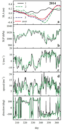
Figure 2.
Time series of (a) SLA at pixels 1–3 and SLA averaged over the area indicated in Figure 1. (b) The sea level pressure (SLP) at locations 1 and 2. (c) The U component of wind at locations 1 and 2. (d) The wind speed at locations 1 and 2. (e) The wind direction at locations 1 and 2. Data are presented for MBI in 2014.
Thus, the combined influence of high air pressure and easterly winds caused the outflow of water and the lowering of the mean sea level in the Baltic Proper. The time progression of sea level is illustrated in Figure 2a. The solid black line for pixel #1 is located in the North Sea near Skagerrak, dashed blue and green lines are for pixels #2 and #3, respectively, while the red line shows changes in SLA anomalies averaged over the area located in Baltic Proper (see Figure 1). There are significant differences in SLA between different locations.
In Figure 3, maps of SLA and SLP are displayed for the MBI event in 2014. Black crosses indicate the specific pixels discussed in the text (and listed in Table 2). Data are available with daily resolution. However, because of limited space in the paper, we displayed selected days only. Figure 3a,b show the SLA and SLP maps for day 329 (25 November), which represents the situation during the outflow phase. We note that, during that time, the SLP was relatively high over the entire area of the Baltic Sea (1020 hPa and more), while the SLA values were negative. On day 340 (5 December, Figure 3c,d) representing the situation at the beginning of the inflow phase, SLAs were about −0.4 m. After that time, SLAs increased. On day 361 (Figure 3d,g), just after the inflow ended, SLAs reached about +0.5 m almost everywhere in the Baltic Proper.
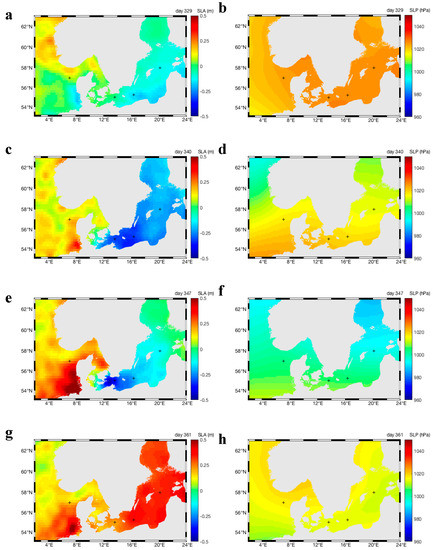
Figure 3.
Maps of sea level anomalies (column on the left side) and atmospheric pressure at sea level (column on the right side) during the MBI event in 2014. Data are shown for selected days (329, 340, 347, and 361). Crosses indicate pixels 1–4.
Changes in sea level during 2014 MBI can be evaluated in Figure 4, where we compared time series data of SLA at four selected pixels and SLA averaged over the Baltic Proper with time series of tide gauge data at several stations. The sea level at tide gauge stations is quite variable. The displayed tide gauge data have hourly resolution, while the SLA data have daily resolution. It is, therefore, expected that the tide gauge data show more variability on a short time scale than the SLA data. Nevertheless, even if the stations Landsort Norra, Stockholm, and Visby are located near each other, we can note clear differences in the sea level recorded at these stations. The differences are even larger if we consider stations that are located at larger distances from each other (Figure 4d). Tide gauges are located on the coastlines, and these observations always include coastal effects such as waves and wind surges. Storm surges in the Baltic Sea are significant, and depend on the local coastal topography and specific spatial distribution of meteorological forcing. Many problems (also those related to tectonic uplift, regional postglacial rebound) associated with the use of tide gauge data to estimate changes in the volume of water in the Baltic Sea can be avoided with application of satellite altimetry. So far, though, the MBIs were not discussed in the literature in the context of satellite data. In this paper, we are filling this gap. The advantage of using satellite sea level data is associated with the fact that such data allow us to monitor the entire surface of the Baltic and North Seas. In addition, SLA data used in this paper represent the conditions prevailing in the open sea. The disadvantage is that satellite data have poorer temporal resolution than the in situ data.
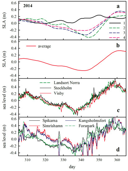
Figure 4.
Time series of SLA compared with tide gauge data at selected stations during Major Baltic Inflow in 2014: (a) time series of SLA at pixels 1–4. (b) Time series of SLA averaged over the Baltic Proper. (c) Time series of the sea level measured at Landsort Norra, Stockholm, and Visby. (d) Time series of the sea level measured at Simrishamn, Kungsholmsfort, and Forsmark. See Table 2 for geographical coordinates of the stations.
The Leibniz Institute for Baltic Sea Research in Warnemünde, Germany (IOW) provides an in-depth annual assessment of hydrographic conditions in the Baltic Sea [14,15,16]. This assessment is based on extensive data from research cruises and autonomous stations (the German MARNET monitoring network, tide gauges of the Swedish Meteorological and Hydrological Institute, SMHI, and data from the Maritime Office of the Polish Institute of Meteorology and Water Management, IMGW). The reports assess water exchange processes between the Baltic and the North Seas, and deliver information about the MBI events. According to the IOW reports, at least seven MBI events took place during the time interval (1993–2017) considered in our paper. The information about the timing of these MBI events and the volume of water delivered into the Baltic Sea is summarized in Table 3.
Table 3.
Estimates of the volume of water transported into the Baltic Sea during Major Baltic Inflows based on SLA. Column on the right side shows data from the literature.
Figure 5, Figure 6 and Figure 7 exhibit the time-dependent changes in SLA at selected pixels and SLA averaged over the Baltic Proper before and during the MBIs in 1993, 2003, 2011, 2015, and 2016. Accompanying meteorological conditions observed at pixel 1 and 2 are also shown. We can see that, analogously to what was observed for the MBI in 2014 (Figure 2), also in other cases just before a given MBI event, a relatively high SLP was detected. This was followed by a lower SLP during the main inflow phase. However, there is no strict rule regarding the exact values of SLP. For example, during the MBI in 2016 (indicated as MBI 2016A in Figure 7), SLP was quite variable during the pre-inflow and during the inflow phases. In addition, during all MBI events, we observed a change in the dominant wind direction with easterly winds present during the outflow phase and westerly winds prevailing during the main inflow phase. Thus, during all of the analyzed MBIs, there is a general agreement with the characteristic sequence of meteorological conditions described in the literature [2,11].
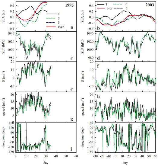
Figure 5.
Time series of (a, b) SLA at pixels 1–3 and SLA averaged over the area indicated in Figure 1. (c, d) Sea level pressure (SLP) at locations 1 and 2. (e, f) U component of wind at locations 1 and 2. (g, h) Wind speed at locations 1 and 2. (i, j) Wind direction at locations 1 and 2. Data are presented for MBIs in 1993 and 2003 in the column on the left and right side, respectively.
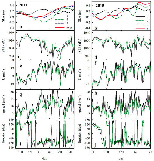
Figure 6.
The same as in Figure 5, but data are presented for MBIs in 2011 (column on the left side) and 2015 (column on the right side).
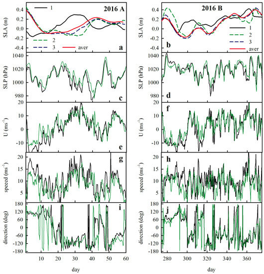
Figure 7.
The same as in Figure 5, but data are presented for MBI in 2016 (column on the left side) and for the barotropic inflow in the fall/winter of 2016 (column on the right side). This event was not classified as the MBI in the IOW reports.
On the other hand, there is also a significant variability in the meteorological conditions if one compares more closely the patterns during different MBI events. To better illustrate this point, we have decided to compare the frequency distributions of meteorological data for each of the events. First, we have defined the outflow and the inflow time intervals based on the observed changes in the mean SLA. The outflow started about 10 to 20 days before the main MBI. It began when the decrease of mean SLA was observed in the Baltic Proper, and lasted until the minimum mean SLA was recorded before the MBI event. We assumed that the inflow phase started after the minimum SLA was recorded and ended when we observed the maximum in SLA time series. Using the data from the outflow and the inflow phases, we have created histograms showing the frequency distribution of SLP (Figure 8) and wind roses (Figure 9 and Figure 10).
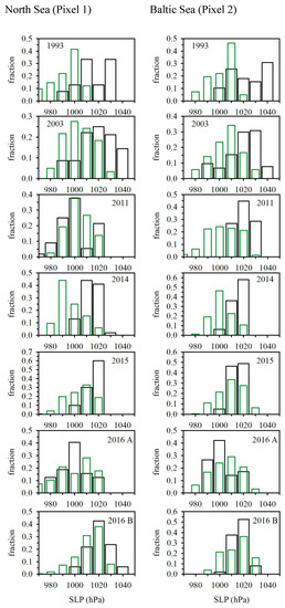
Figure 8.
Frequency distribution of sea level pressure (SLP) at pixel 1 (left side panel) and pixel 2 (right side panel) during inflow events. Data from the outflow phase are shown in black. Data for the inflow phase are plotted in green.
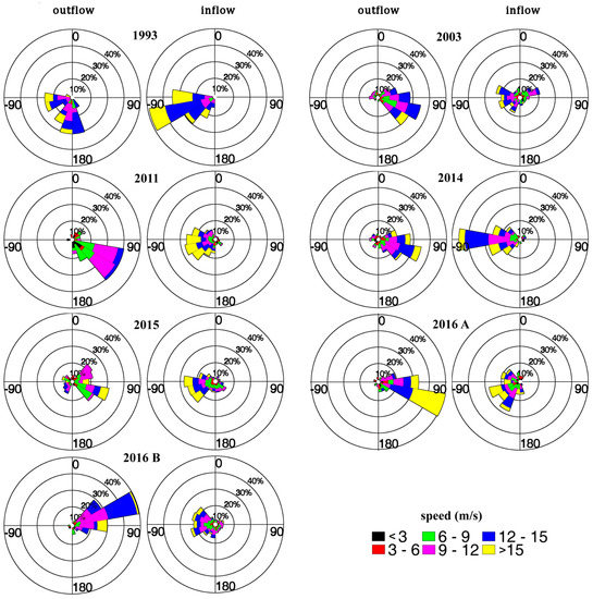
Figure 9.
Wind roses summarizing wind conditions at pixel 1 (North Sea) for different MBI events. Each wind rose shows frequency of occurrence (in %) of different wind directions (according to the meteorological convention) and frequency of occurrence of wind speed values for a given direction. Solid black rings indicate the 10%, 20%, 30%, and 40%. Plots on the left side are for the outflow phase and on the right side for the inflow phase of each MBI event.
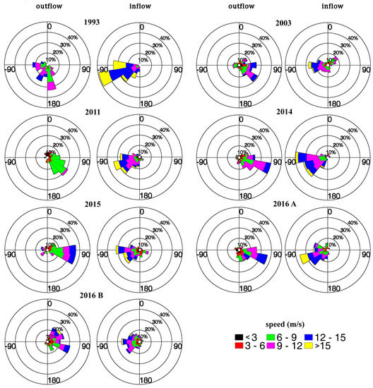
Figure 10.
As in Figure 9, but for pixel 2 (Baltic Sea).
We can see in Figure 8 that the highest SLPs were observed during the MBIs in 1993 and 2003. In 2014, such high SLP values were not observed. However, higher SLP values were recorded during the outflow phase in comparison with the inflow phase. During the spring event of 2016 (marked as 2016A), the SLP influence on the MBI development was most likely less significant than in the other years, since the SLP histogram for the outflow phase does not include very high values. Frequency distributions for wind direction and wind speed during each MBI are summarized in wind roses (Figure 9 and Figure 10). There is a striking difference between wind conditions during the outflow and the inflow phases. Most importantly, there is a significant difference in the dominant wind direction. During the outflow phase, the winds from southeast and south dominated, while, during the inflow phase, westerly winds were the most frequent. If we compare all data for all the MBIs, we note that, in 1993, the wind directions during the outflow phase were more variable and easterly winds were more rare than during outflow time intervals preceding the other MBIs.
On the other hand, the MBI in 1993 was preconditioned by high SLP during the outflow phase. The SLP decreased significantly during the inflow phase and this change in SLP contributed to observed trends in SLA. This MBI was additionally strengthened by favorable high wind speed from the west observed during the inflow phase. The MBI in 1993 was the second most important MBI recorded in our data set. The most prominent MBI according to our analysis was the MBI in 2014. As mentioned before, this MBI was preconditioned by high SLP values during the outflow phase, but these values were not as high as during the 1993 outflow. However, the MBI in 2014 during the outflow phase was accompanied by very strong winds from easterly directions, and this is probably why the SLA reached lower values during the outflow phase of 2014 than in 1993. The role of wind was also relatively important during the outflow phase in 2016A MBI. Strong winds were observed more often during the inflow phase of the MBIs in 1993, 2011, and 2014 than during other events. It is impossible to evaluate the relative importance of specific meteorological conditions for the development of MBIs using simple histograms, but our data underline the fact that there was a significant variability in meteorological conditions accompanying the MBI events. There are also notable differences between the meteorological conditions recorded at the North Sea site and in the Baltic Proper. During some inflow events, the winds at the North Sea site reach higher speeds more often than at the Baltic Sea site, and this most likely also influences the development of the MBI events. More thorough cause- effect analysis of atmospheric forcing on the MBIs should be based on a modeling study and is out of the scope of the present paper.
Figure 11 shows how the SLA patterns during the MBI events compare to the full time series of SLA variability. Time series plotted in Figure 11 include data for pixel 1 (North Sea), pixel 2 (western Baltic Sea), and SLA averaged over the Baltic Proper. It has to be noted that our plots looked exactly the same when we replaced data from pixel 1 with the SLA averaged over 2 × 2 degree area (55–57° N, 4–6° E) in the North Sea (not shown). In Figure 11, the MBI events are highlighted by horizontal blue lines. The characteristic pattern for the MBI involves an initial decrease of the SLA. Usually, during this phase, the SLA decreases more inside the Baltic Sea and less in the North Sea. This is followed by a significant increase of the SLA in the North Sea, with the SLA values inside the Baltic Sea appearing low. This leads to the situation where the SLA values in the North Sea are larger than the SLA inside the Baltic Sea. Lastly, at the end of the MBI, the SLA in the North and Baltic Seas become very close in values. Later, the SLA in the Baltic Sea can increase even more. Thus, the presence of the MBI can be traced on the SLA time series as an event when there is a significant discrepancy between the SLA in the North Sea and in the Baltic Sea.
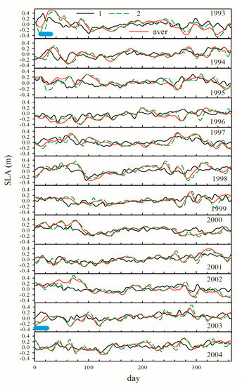
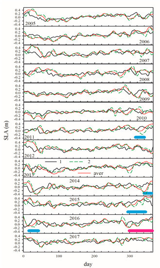
Figure 11.
Time series of SLA in years 1993–2017. Data for pixel 1 (North Sea) are shown as a solid black line, for pixel 2 as a dashed green line, and for the mean SLA in the Baltic Sea proper as a red line. Horizontal thick blue lines indicate MBI events. The inflow event during the fall of 2016 has been marked in red, which has not been classified in IOW reports as the MBI.
In Figure 11, there are also smaller events, when minor inflows due to the sea level difference could have most likely taken place. However, these events have not been classified as the Major Baltic Inflows, because they were too small. On the other hand, we note synchronous changes in the SLA patterns present in the time series from both the Baltic Sea and the North Sea. Such changes are in agreement with the fact that SLA in both seas undergo a similar annual pattern of variability and are also significantly influenced by the zonal wind component, which changes on a synoptic time scale [27,30].
4. Summary and Conclusions
Variability of the sea level in the North and Baltic Seas enforced by weather patterns affects the intensity of water exchange between these seas. Transfer of salty water from the North Sea is very important for the hydrography of the Baltic Sea. It was studied for many years. Particular attention was paid to events associated with transfers of large volumes of salty water including the Major Baltic Inflows [9,17,18,19,37]. In recent years, the society, politicians, and scientists have become worried that the ‘environmental health’ of the Baltic Sea is in an inferior condition. Reports describing the increase of the ‘dead bottom areas’ were published [38]. It is, therefore, crucial to advance our understanding of the dynamic connections of this marine system with the external ocean, and to achieve a better perception of the possible cause-effect relationships between sea level variability, its impact on water exchange with the North Sea, and their significance for the ecological status of the Baltic Sea.
MBI events are unpredictable and of relatively short duration. Therefore, it is very challenging to collect data sets documenting in full detail the temporal development of such events based on oceanographic cruises. With the advent of autonomous oceanographic instrumentation, long-term continuous hydrographic data covering the MBI events were collected [9]. Since 1993, several MBIs were recorded where the most prominent one was in 2014. Based on field data, detailed analyses of the MBIs in 1993 [12], 2003 [4,5,39], and 2014 [11,17,18,34,40] were published. Until now, in research about the MBIs, the tide gauge data were used to represent the large-scale sea level variability in the Baltic Sea. In the present paper, we carried out a similar analysis using remote sensing altimetry data. Our research is based on data that systematically cover the area of the entire Baltic Sea, but were not explored before in the context of the MBIs.
We have shown that remote sensing should be used as a complementary source of information about the MBI events. The advantage of using such data is that large-scale spatial information about SLA is available with daily resolution. In contrast, the oceanographic cruise data, the mooring or tide gauge data provide information with poor spatial resolution. In addition, traditional datasets from tide gauges display a substantial spatial heterogeneity, which reflects the diverse local and regional processes impacting tide gauge records. It is, therefore, exciting to apply more modern satellite altimetry data in the research on the MBIs. In the near future, we expect that a new generation of satellite altimeters and improved methods of altimetry data processing will have even better capabilities to deliver improved altimetry data sets for research in the Baltic Sea. This opens the possibility that, in the future, a near real-time monitoring system of the Baltic Sea environment will include satellite altimetry observations. In addition to the MBIs, which happen rarely and at irregular intervals of time (every few years), there are also more frequent but weak inflows of salty water into the Baltic Sea. They can be overlooked or are underestimated with traditional observational techniques. These smaller inflows have low impact on the status of the deep waters. They cannot displace the bottom water masses and do not influence conditions significantly for the organisms living in the deep basins of the sea. However, these minor inflows most likely have the capability to precondition the deep-water masses and facilitate the spreading of the water brought into the Baltic Sea during the MBI events. These smaller events have also undoubtedly significant influence on the salinity of the Baltic Sea water at intermediate depths. Satellite observations can be useful for observations of these inflows as well.
Summarizing the most important findings:
- We have shown that satellite altimetry data can be used to monitor Major Baltic Inflows.
- MBI events correspond to specific patterns in SLA time series that include asynchronous change in SLA in the North and Baltic Seas. That is, after the initial decrease in SLA observed in both seas during the outflow phase, the SLA increases more rapidly in the North Sea than in the Baltic Sea during the inflow phase. With progression of the inflow, the SLA returns to normal values and usually increases above the average level in the Baltic Sea.
- Our analysis allowed us to approximately quantify the volumes of water transported into the Baltic Sea during the MBIs observed in the time interval from 1993 to 2017. The results were similar to the values published in the past in the literature and based on in situ data.
- It was confirmed that, during the investigated time interval, the largest MBI happened in 2014 and the second largest happened in 1993.
- Based on the analysis of SLA and meteorological data from ERA Interim, we confirmed that MBIs are linked to a characteristic sequence of weather conditions, as described in the past.
- Even if the general pattern is similar, there is a significant variability of meteorological conditions forcing different MBI events.
- Most of the time, when the MBIs are not present, the SLA changes in both seas are almost synchronous. However, we also noted some events with similar SLA patterns as those observed during the MBIs, but with a smaller range of SLA variability. These patterns most likely indicate small barotropic inflows.
Author Contributions
Conceptualization, M.S. Formal analysis, M.S. and P.A. Methodology, M.S. Visualization, M.S. and P.A. Writing—original draft, M.S.
Funding
The National Science Center in Poland (contract number: 2017/25/B/ST10/00159 entitled: “Numerical simulations of biological-physical interactions and phytoplankton cycles in the Baltic Sea”) funded this research. Partial support comes from the statutory funds of the Institute of Oceanology of the Polish Academy of Sciences (IO PAN). A scholarship from the Leading National Research Center (KNOW), obtained by the Center for Polar Studies in Poland, also supported P.A.
Acknowledgments
The authors are grateful to all the persons involved in the programs providing free access to the data sets used in this study. The altimeter data were processed by Ssalto/Duacs and distributed by the Copernicus Marine and Environment Monitoring Service (CMEMS) (http://marine.copernicus.eu). The meteorological reanalysis data were obtained from the ERA-Interim project at the European Center for Medium-Range Weather Forecasts (ECMWF) (http://apps.ecmwf.int/datasets/data/interim-full-daily/). Tide gauge and river runoff data were downloaded from the SMHI open data service.
Conflicts of Interest
The authors declare no conflict of interest.
References
- Leppäranta, M.M.; Myrberg, K. Physical Oceanography of the Baltic Sea. Springer-Praxis Book Series in Geophysical Sciences; Springer: Chichester, UK, 2009; p. 378. [Google Scholar]
- Matthäus, W.W.; Franck, H. Characteristics of major Baltic inflows—A statistical analysis. Cont. Shelf Res. 1992, 12, 1375–1400. [Google Scholar] [CrossRef]
- Sellschopp, J.J.; Arneborg, L.L.; Knoll, M.M.; Fiekas, V.V.; Gerdes, F.F.; Burchard, H.H.; Lass, H.U.U.; Mohrholz, V.V.; Umlauf, L. Direct observations of a medium-intensity inflow into the Baltic Sea. Cont. Shelf Res. 2006, 26, 2393–2414. [Google Scholar] [CrossRef]
- Feistel, R.R.; Nausch, G.G.; Matthäus, W.W.; Hagen, E. Temporal and spatial evolution of the Baltic deep water renewal in spring 2003. Oceanologia 2003, 45, 623–642. [Google Scholar]
- Feistel, R.R.; Hagen, E.E.; Nausch, G. Unusual Baltic inflow activity in 2002–2003 and varying deep-water properties. Oceanologia 2006, 48, 21–35. [Google Scholar]
- Reissmann, J.H.H.; Burchard, H.H.; Feistel, R.R.; Hagen, E.E.; Lass, H.U.U.; Mohrholz, V.V.; Nausch, G.G.; Umlauf, L.L.; Wieczorek, G. Vertical mixing in the Baltic Sea and consequences for eutrophication—A review. Prog. Oceanogr. 2009, 82, 47–80. [Google Scholar] [CrossRef]
- Schinke, H.H.; Matthäus, W. On the causes of major Baltic inflows - an analysis of long time series. Cont. Shelf Res. 1998, 18, 67–97. [Google Scholar] [CrossRef]
- Matthäus, W. The history of investigation of salt water inflows into the Baltic Sea—From the early beginning to recent results. Meereswiss. Ber. 2006, 65, 1–73. [Google Scholar]
- Matthäus, W.W.; Nehring, D.D.; Feistel, R.R.; Nausch, G.G.; Mohrholz, V.V.; Lass, H.-U. The inflow of highly saline water into the Baltic Sea. In State and Evolution of the Baltic Sea, 1952–2005; Feistel, R.R., Nausch, G.G., Wasmund, N., Eds.; Wiley: Hoboken, NJ, USA, 2008; pp. 265–309. [Google Scholar]
- Nehring, D.D.; Matthäus, W.W.; Lass, H.-U.U.; Nausch, G.G.; Nagel, K. The Baltic Sea in 1995—Beginning of a new stagnation period in its central Baltic deep waters and decreasing nutrient load in its surface layer. Dtsch. Hydrogr. Z. 1995, 47, 319–327. [Google Scholar] [CrossRef]
- Mohrholz, V.V.; Naumann, M.M.; Nausch, G.G.; Krüger, S.S.; Gräwe, U. Fresh oxygen for the Baltic Sea—An exceptional saline inflow after a decade of stagnation. J. Mar. Syst. 2015, 148, 152–166. [Google Scholar] [CrossRef]
- Matthäus, W.W.; Lass, H.U. The recent salt inflow into the Baltic Sea. J. Phys. Oceanogr. 1995, 25, 280–286. [Google Scholar] [CrossRef]
- Feistel, R.R.; Nausch, G.G.; Matthäus, W.W.; Łysiak-Pastuszak, E.E.; Seifert, T.T.; Sehested Hansen, I.I.; Mohrholz, V.V.; Krüger, S.S.; Buch, E.E.; Hagen, E. Background Data to the Exceptionally Warm Inflow into the Baltic Sea in late Summer of 2002; Technical Report; Leibniz Institute for Baltic Sea Research: Rostock, Germany, 2004. [Google Scholar]
- Nausch, G.G.; Naumann, M.M.; Umlauf, L.L.; Mohrholz, V.V.; Siegel, H. Hydrographisch-hydrochemische Zustandseinschätzung der Ostsee 2013. Meereswiss. Ber. Warnemünde 2014, 93. [Google Scholar] [CrossRef]
- Nausch, G.G.; Naumann, M.M.; Umlauf, L.L.; Mohrholz, V.V.; Siegel, H.H.; Schulz-Bull, D. Hydrographic-hydrochemical assessment of the Baltic Sea 2015. Meereswiss. Ber. Warnemünde 2016, 101. [Google Scholar] [CrossRef]
- Naumann, M.M.; Umlauf, L.L.; Mohrholz, V.V.; Kuss, J.J.; Siegel, H.H.; Waniek, J.J.; Schulz-Bull, D. Hydrographic-hydrochemical assessment of the Baltic Sea 2016. Meereswiss. Ber. Warnemünde 2017, 104. [Google Scholar] [CrossRef]
- Holtermann, P.L.L.; Prien, R.R.; Naumann, M.M.; Mohrholz, V.V.; Umlauf, L. Deepwater dynamics and mixing processes during a major inflow event in the central Baltic Sea. J. Geophys. Res. Oceans 2017, 122, 6648–6667. [Google Scholar] [CrossRef]
- Neumann, T.T.; Radtke, H.H.; Seifert, T. On the importance of Major Baltic Inflows for oxygenation of the central Baltic Sea. J. Geophys. Res. 2017, 122, 1090–1101. [Google Scholar] [CrossRef]
- Hagen, E.E.; Feistel, R. Spreading of Baltic deep water: A case study for the winter 1997–1998. Meereswiss. Ber. 2001, 45, 99–133. [Google Scholar]
- Umlauf, L.L.; Arneborg, L. Dynamics of rotating shallow gravity currents passing through a channel. Part I: Observation of transverse structure. J. Phys. Oceanogr. 2009, 39, 2385–2401. [Google Scholar] [CrossRef]
- Liblik, T.T.; Naumann, M.M.; Alenius, P.P.; Hansson, M.M.; Lips, U.; Nausch, G.; Tuomi, L.; Wesslander, K.; Laanemets, J.; Viktorsson, L. Propagation of impact of the recent Major Baltic Inflows from the Eastern Gotland Basin to the Gulf of Finland. Front. Mar. Sci. 2018, 5, 222. [Google Scholar] [CrossRef]
- Ekman, M. The Changing Level of the Baltic Sea during 300 Years: A Clue to Understanding the Earth; Summer Institute for Historical Geophysics: Åland Islands, Finland, 2009; p. 155. ISBN 978- 952-92-5241-1. [Google Scholar]
- Nerem, R.S.; Chambers, D.P.; Choe, C.; Mitchum, G.T. Estimating mean sea level change from the TOPEX and Jason altimeter missions. Mar. Geod. 2010, 33, 435–446. [Google Scholar] [CrossRef]
- Le Provost, C. Ocean tides. In Satellite Altimetry and Earth Sciences: A Handbook of Techniques and Applications; Fu, L.-L., Cazenave, A., Eds.; Academic Press: San Diego, CA, USA, 2000; pp. 267–304. ISBN 0122695453. [Google Scholar]
- Stramska, M.; Chudziak, N. Recent multiyear trends in the Baltic Sea level. Oceanologia 2013, 55, 319–337. [Google Scholar] [CrossRef]
- Stramska, M.; Kowalewska-Kalkowska, H.; Świrgoń, M. Seasonal variability of the Baltic Sea level. Oceanologia 2013, 55, 787–807. [Google Scholar] [CrossRef]
- Stramska, M. Temporal variability of the Baltic Sea level based on satellite observations. Estuar. Coast. Shelf Sci. 2013, 133, 244–250. [Google Scholar] [CrossRef]
- Passaro, M.; Cipollini, P.; Benveniste, J. Annual sea level variability of the coastal ocean: The Baltic Sea-North Sea transition zone. J. Geophys. Res. Oceans 2015, 120, 3061–3078. [Google Scholar] [CrossRef]
- Xu, Q.; Cheng, Y.; Plag, H.P.; Zhang, B. Investigation of sea level variability in the Baltic Sea from tide gauge, satellite altimeter data, and model reanalysis. Int. J. Remote Sens. 2015, 36, 2548–2568. [Google Scholar] [CrossRef]
- Cheng, Y.; Xu, Q.; Li, X. Spatio-Temporal Variability of Annual Sea Level Cycle in the Baltic Sea. Remote Sens. 2018, 10, 528. [Google Scholar] [CrossRef]
- Dee, D.P.; Uppala, S.M.; Simmons, A.J.; Berrisford, P.; Poli, P.; Kobayashi, S.; Andrae, U.; Balmaseda, M.A.; Balsamo, G.; Bauer, P.; et al. The ERA-Interim reanalysis: Configuration and performance of the data assimilation system. Q. J. R. Meteorol. Soc. 2011, 137, 533–597. [Google Scholar] [CrossRef]
- Arheimer, B. E-HypeWeb: Service for water and climate information—And future hydrological collaboration across Europe. In Environmental Software Systems. Frameworks of eEnvironment, IFIP Advances in Information and Communication Technology; Hřebíček, J., Schimak, G., Denzer, R., Eds.; Springer: Berlin, Germany, 2011; Volume 359, pp. 657–666. [Google Scholar]
- Donnelly, C.H.; Andersson, J.C.M.; Arheimer, B. Using flow signatures and catchment similarities to evaluate the E-HYPE multi-basin model across Europe. Hydrol. Sci. J. 2016, 61, 255–273. [Google Scholar] [CrossRef]
- Mohrholz, V. Major Baltic Inflow Statistics—Revised. Front. Mar. Sci. 2018, 5, 384. [Google Scholar] [CrossRef]
- Gräwe, U.; Naumann, M.; Mohrholz, V.; Burchard, H. Anatomizing one of the largest saltwater inflows into the Baltic Sea in December 2014. J. Geophys. Res. Oceans 2015, 120, 7676–7697. [Google Scholar] [CrossRef]
- Wunsch, C.; Stammer, D. Atmospheric loading and the oceanic “inverted barometer” effect. Rev. Geophys. 1997, 35, 79–107. [Google Scholar] [CrossRef]
- Gustafsson, B.G.; Stigebrandt, A. Dynamics of nutrients and oxygen/hydrogen sulfide in the Baltic Sea deep water. J. Geophys. Res. 2007, 112, G02023. [Google Scholar] [CrossRef]
- Pawlak, J.; Laamanen, M.; Andersen, J.H. Eutrophication in the Baltic Sea—An integrated thematic assessment of the effects of nutrient enrichment and eutrophication in the Baltic Sea region. Balt. Sea Environ. Proc. 2009, 115B, 148. [Google Scholar] [CrossRef]
- Piechura, J.; Beszczyńska-Möller, A. Inflow waters in the deep regions of the southern Baltic Sea—Transport and transformations. Oceanologia 2004, 46, 113–141. [Google Scholar]
- Rak, D. The inflow in the Baltic Proper as recorded in January–February 2015. Oceanologia 2016, 58, 241–247. [Google Scholar] [CrossRef]


© 2019 by the authors. Licensee MDPI, Basel, Switzerland. This article is an open access article distributed under the terms and conditions of the Creative Commons Attribution (CC BY) license (http://creativecommons.org/licenses/by/4.0/).