Hyperspectral Unmixing with Gaussian Mixture Model and Low-Rank Representation

Abstract

Gaussian mixture model (GMM) has been one of the most representative models for hyperspectral unmixing while considering endmember variability. However, the GMM unmixing models only have proper smoothness and sparsity prior constraints on the abundances and thus do not take into account the possible local spatial correlation. When the pixels that lie on the boundaries of different materials or the inhomogeneous region, the abundances of the neighboring pixels do not have those prior constraints. Thus, we propose a novel GMM unmixing method based on superpixel segmentation (SS) and low-rank representation (LRR), which is called GMM-SS-LRR. we adopt the SS in the first principal component of HSI to get the homogeneous regions. Moreover, the HSI to be unmixed is partitioned into regions where the statistical property of the abundance coefficients have the underlying low-rank property. Then, to further exploit the spatial data structure, under the Bayesian framework, we use GMM to formulate the unmixing problem, and put the low-rank property into the objective function as a prior knowledge, using generalized expectation maximization to solve the objection function. Experiments on synthetic datasets and real HSIs demonstrated that the proposed GMM-SS-LRR is efficient compared with other current popular methods.

1. Introduction

In the last few decades, Hyperspectral image (HSI) has received considerable attention in the field of earth observation and geoinformation science. With the wealth of spatial and spectral information, HSI has been successfully applied in many applications, such as spectral unmixing, environment monitoring, matching and object classification [1,2,3,4,5,6,7,8]. However, due to the low spatial resolution of current HSI sensors and the mixed effects of the ground surface, these factors will seriously affect the accurate interpretation of the image content. In this case, spectral unmixing (SU) problem has become a major issue for the deep development of HSI.

The information of hyperspectral images can be simplified by the linear mixing model (LMM), which assumes that the physical region corresponding to a pixel contains several pure materials. Hence, the observed spectra ${\mathbf{y}}_n\in {\mathbb{R}}^B,n=1,\dots ,N$ (B is the number of wavelengths and N is the number of pixels) is a (non-negative) linear combination of the pure material (called endmember) spectra $m_j\in {\mathbb{R}}^B,j=1,\dots ,M$ (M is the number of endmembers) [9], i.e.,

$${\mathbf{y}}_n={\displaystyle \sum _{j=1}^M}{\mathbf{m}}_j{\alpha }_{nj}+{\mathbf{n}}_n,\mathrm{s}.\mathrm{t}.{\alpha }_{nj}\ge 0,{\displaystyle \sum _{j=1}^M}{\alpha }_{nj}=1,$$

(1)

where ${\alpha }_{nj}$ is the proportion (called abundance) for the jth endmember at the nth pixel (with the positivity and sum-to-one constraint) and ${\mathbf{n}}_n\in {\mathbb{R}}^B$ is additive noise. Here, the endmember set ${\mathbf{m}}_j:j=1,\dots ,M$ is fixed for all the pixels. Many endmember detection algorithms are under the pixel purity assumption to extract the pure endmembers, such as the pixel purity index [10], successive projection algorithm [11], and vertex component analysis (VCA) [12]. Other algorithms assume that all the pixels lie in a convex hull in a high-dimensional subspace: N-Finder [13] and iterative constrained endmembers (ICE) [14]. In our proposed abundance estimation method, the pure endmembers are assumed to be known or they can be identified from the target image by one of these endmember detection techniques.

However, in practice, the LMM may not be an appropriate model in many real scenarios. Even for a pure pixel that only contains one material, over the whole image its spectrum may not be consistent. This is due to several factors such as intrinsic variability, atmospheric conditions and topography. Equation (1) can be generalized to a more abstract form, ${\mathbf{y}}_n=S\left({\mathbf{m}}_j,{\alpha }_{nj}:j=1,\dots ,M\right)$, which is called nonlinear mixing models (NLMMs). For example, in [15], the generalized bilinear model (GBM) generalizes the LMM by introducing bilinear terms to handle the vegetation case with taking into account the multipath effects. In that case, various representative abundance estimation algorithms have been proposed based on different nonlinear model assumptions, such as least squares [16], kernel-based least squares [17,18], and Bayesian methods [15]. A panoply of nonlinear models can be found in the review article [19]. The reason we note those models is that the endmember set is still assumed to be fixed.

Although NLMM models have abounded recently, it is still not appropriate to account for all the scenarios. LMM has also been widely used due to its simplicity and physical meaning. To model real scenarios more accurately, researchers have taken another route by generalizing Equation (1) to

$${\mathbf{y}}_n={\displaystyle \sum _{j=1}^M}{\mathbf{m}}_{nj}{\alpha }_{nj}+{\mathbf{n}}_n,\mathrm{s}.\mathrm{t}.{\alpha }_{nj}\ge 0,{\displaystyle \sum _{j=1}^M}{\alpha }_{nj}=1,$$

(2)

where ${\mathbf{m}}_{nj}\in {\mathbb{R}}^B:j=1,\dots ,M,n=1,\dots ,N$. We note that the endmember set in that case is not fixed and the endmember spectra could be different for each pixel ${\mathbf{y}}_n$. This is called endmember variability. Given ${\mathbf{y}}_n$, inferring ${\mathbf{m}}_{nj},{\alpha }_{nj}$ is a much more difficult problem than inferring ${\mathbf{m}}_j,{\alpha }_{nj}$ in Equation (1).

In the review paper [20], the methods taking into account the endmember variability can be expressed in two categories: (1) endmembers represented as a discrete set; or (2) endmembers represented using a continuous distribution. In the first category, the endmember spectra are modeled as a series of spectra clusters, and expressed as discrete sets in mathematical form. The multiple endmember spectral mixture analysis (MESMA) is one of the widely used methods of this category [21], which tries every endmember combination to search the minimum mean square error in the discrete set as the final calculation result. There are many variations to the original MESMA, such as the multiple-endmember linear spectral unmixing model (MELSUM) [22], Auto-Monte Carlo Unmixing (AutoMCU) [23,24] and the Bayesian spectral mixture analysis (BSMA) [25]. Besides those variants, there are also some other set based methods, e.g., endmember bundles [26] and band weighting or transformation approaches [27,28]. However, those methods mentioned above have a common disadvantage that, when the spectral library is large, their complexity will increase exponentially, resulting in extreme computational inefficiency difficulties.

The second category usually takes statistical method to model the endmember distribution. Specifically, it is assumed that the endmembers of each pixel are sampled from a probability distribution, and hence embrace large libraries while being numerically tractable. In [29], Eches et al. proposed the normal compositional model (NCM). This model is the early representative work in this direction, which assumes the endmembers for each pixel are sampled from unimodal Gaussian distribution (primarily due to mathematical simplicity). Due to the complexity of the model’s prior knowledge and hyperparameters, the maximum a posteriori (MAP) constructed is often a non-convex function. Then, NCM uses different optimization approaches, such as expectation maximization [30], sampling method [31], and particle swarm optimization [32], to determine the hyperparameters. However, the NCM allows for endmember samples to range outside the interval of $[0,1]$ and in the real scenarios the endmember distribution could be skewed. Hence, Du et al. proposed a Beta compositional model (BCM) to model the endmember variability in the HSI unmixing [33]. However, the true distribution may not be well approximated by either a Gaussian or Beta distribution. In that case, Zhou et al. proposed the Gaussian mixture model (GMM) to solve the LMM by considering endmember variability [34]. GMM method assumes that the endmember ${\mathbf{m}}_{nj}$ follows the GMM distribution and noise ${\mathbf{n}}_n$ follows the Gaussian distribution: $p\left({\mathbf{n}}_n\right):=\mathcal{N}\left({\mathbf{n}}_n\right|0,\mathbf{D})$, where $\mathbf{D}$ is the noise covariance matrix, and with proper abundances constraint under the Bayesian framework to lead the conditional density function to a standard MAP problem.

The performance of those methods in this category is often dependent on the initial value of parameters, but does not rely on the large-scale spectral database, which is the research hotspot for the endmember variability problem. However, neither method mentioned above takes into account the possible spatial correlation between local pixels. Researchers in [2,35,36] proved that the spatial correlations between the observed pixels can enhance the performance of spectral unmixing. On the other hand, this strategy has great advantages of easily generalizing the Bayesian algorithms, which is introduced in [37,38]. In that vein, in an attempt to achieve better abundance estimation results, Zhou’s model (GMM) [34] uses the proper smoothness and sparsity prior constraints on the abundances, while Iordache et al. [39] tried to find the minimum difference of the abundance between the adjacent pixels by the total variation (TV) constraint. However, those prior constraint assumptions require a rather strict assumption that the abundance of the local pixel should be piecewise smooth, which means that the mixing pixel and its associated abundance should be similar for the adjacent pixels. When the pixels lie on the boundaries of different materials or the inhomogeneous region, the abundances in the neighboring pixels do not have those prior constraints. Driven by those considerations, to further exploit the spatial data structure, we take superpixel segmentation (SS) in the first principal component of HSI to get the homogeneous regions. Then, the hyperspectral image to be unmixed is partitioned into several homogeneous regions (or classes) in which the abundance vector has the same first and second order statistical moments (means and covariances). The shape and size can be accustomed on the basis of different spatial structures, and each superpixel can be seen as a non-overlapping region.

Furthermore, in those homogeneous regions, there is a high degree of correlation among the spectral signatures of the neighboring pixels. The high spatial similarity usually implies the low-rank property in the abundance map. Qu et al. [40] proved that the abundance matrix has low-rank property in homogeneous region and constructed an unmixing model by using low-rank property to verify the effectiveness in homogeneous region unmixing. Giampouras et al. [36] proposed a novel low-rank representation (LRR) for HSI unmixing, which jointly obtains a representation for all the data under a global lowest rank constraint. In that vein, we take LRR to further exploit the spatial information between the local pixels in the homogeneous region, using the Bayesian framework to construct the objective function together seeking the lowest rank.

Thus, in this paper, in an attempt to achieve better abundance estimation performance and fully consider the possible spatial correlation between local pixels, we propose a novel GMM unmixing method based on SS and LRR, which is called GMM-SS-LRR. Firstly, we adopt the SS algorithm to cut the HSI into different regions. In these regions, pixels are highly spatial correlated, the mixing pixel and its associated abundance should be similar for the adjacent pixels and the abundance map has low-rank property. Secondly, considering the endmember variability phenomenon, under the Bayesian framework, we use GMM to formulate the unmixing problem, and put the low-rank property into the objective function as a prior knowledge. Finally, we use generalized expectation maximization (GEM) to solve the objective function [41].

In summary, the main contribution in this paper are two folds:

(1) We take SS in the first principal component of HSI to get the homogeneous regions, which can help the GMM method make pixels and their associated abundances similar for the adjacent pixels, since directly using the GMM method to unmixing will make the estimated distribution of the clusters cannot fit the ground truth well and using SS can enhance the performance of the endmember estimation.

(2) We take LRR for the abundance estimation problem, which can further exploit the spatial information between the local pixels. Because after taking SS, the regions will be homogeneous, and the high spatial correlation of the data implies the low-rank property of the abundance matrix, using the LRR property can better capture the spatial data structure by seeking the lowest rank representation, and also get better abundance estimation.

The rest of this paper is structured as follows. In Section 2, we briefly introduce the related GMM method. In Section 3, we describe the proposed model GMM-SS-LRR and the GEM for solving and optimization are introduced. In Section 4, we evaluate the performances of the proposed GMM-SS-LRR and the compared state-of-the-art algorithms on the synthetic datasets and real HSIs. We conclude this paper in Section 5.

2. Related Models

Since the proposed model is closely related with the GMM method, we briefly introduce the GMM in this section.

GMM method [34] is an LMM by considering the endmember variability, use a mixture of Gaussians to approximate any distribution of the endmember and can be classified in the second category mentioned above (endmembers represented using a continuous distribution). GMM model assumes the endmember $p\left({\mathbf{m}}_{nj}\right)$ follows a mixture of Gaussians, and has the density function as follows:

$$p\left({\mathbf{m}}_{nj}\right|\mathbf{\Theta }):=f_{{\mathbf{m}}_j}\left({\mathbf{m}}_{nj}\right)={\displaystyle \sum _{k=1}^{K_j}}{\pi }_{jk}\mathcal{N}\left({\mathbf{m}}_{nj}\right|{\mathit{\mu }}_{jk},{\mathbf{\Sigma }}_{jk}),$$

(3)

subject to ${\pi }_{jk}\ge 0,{\sum }_{k=1}^{K_j}{\pi }_{jk}=1$, with $K_j$ being the number of components, ${\pi }_{jk}$$({\mathit{\mu }}_{jk}\in {\mathbb{R}}^B)$ or ${\mathbf{\Sigma }}_{jk}\in {\mathbb{R}}^{B\times B}$ being the weight (mean or covariance matrix) of its kth Gaussian component, $\mathbf{\Theta }:={\pi }_{jk},{\mathit{\mu }}_{jk},{\mathbf{\Sigma }}_{jk}:j=1,\dots ,M,k=1,\dots ,K_j,{\mathbf{m}}_{nj}:j=1,\dots ,M$ are independent. The noise ${\mathbf{n}}_n$ also follows the Gaussian distribution, which has the density function $p\left({\mathbf{n}}_n\right):=\mathcal{N}\left({\mathbf{n}}_n\right|0,\mathbf{D})$, where $\mathbf{D}$ is the noise covariance matrix and then obtains the distribution of ${\mathbf{y}}_n$ by the equation ${\mathbf{y}}_n={\sum }_{j=1}^M{\mathbf{m}}_{nj}{\alpha }_{nj}+{\mathbf{n}}_n$, which turns out to be another mixture of Gaussians, we can obtain the density function of ${\mathbf{y}}_n$ as follows:

$$p\left({\mathbf{y}}_n\right|{\mathit{\alpha }}_n,\mathbf{\Theta },\mathbf{D})=\sum _{\mathbf{k}\in \mathcal{K}}{\pi }_{\mathbf{k}}\mathcal{N}\left({\mathbf{y}}_n|{\mathit{\mu }}_{n\mathbf{k}},{\mathbf{\Sigma }}_{n\mathbf{k}}\right),$$

(4)

where $\mathcal{K}:=\left\{1,\dots ,K_1\right\}\times \left\{1,\dots ,K_2\right\}\times \dots \times \left\{1,\dots ,K_M\right\}$ is the Cartesian product of the M index sets, $\mathbf{k}$: = $(k_1,\dots ,k_M)\in \mathcal{K},{\pi }_{\mathbf{k}}\in \mathbb{R},{\mathbf{\Sigma }}_{n\mathbf{k}}\in {\mathbb{R}}^{B\times B}$, are defined by:

$${\pi }_{\mathbf{k}}:={\displaystyle \prod _{j=1}^M}{\pi }_{j{k}_j},{\mathit{\mu }}_{n\mathbf{k}}:={\displaystyle \sum _{j=1}^M}{\alpha }_{nj}{\mathit{\mu }}_{j{k}_j},{\mathbf{\Sigma }}_{n\mathbf{k}}:={\displaystyle \sum _{j=1}^M}{\alpha }_{nj}^2{\mathbf{\Sigma }}_{j{k}_j}+\mathbf{D}.$$

(5)

More specifically, in the prior of the abundances of $p\left(\mathbf{A}\right)$, Zhou’s model [34] assumes the abundances $\mathbf{A}$ have the proper smoothness and sparsity prior constraints. The density function of the abundances $\mathbf{A}$ can be generalized as follows:

$$p\left(\mathbf{A}\right)\propto exp\left\{-\frac{{\beta }_1}{2}\mathrm{Tr}\left({\mathbf{A}}^T\mathbf{LA}\right)+\frac{{\beta }_2}{2}\mathrm{Tr}\left({\mathbf{A}}^T\mathbf{A}\right)\right\},$$

(6)

where $\mathbf{L}$ is a graph Laplacian matrix constructed from $w_{nm},n,m=1,\dots ,N$ with $w_{nm}=e^{\Vert {\mathbf{y}}_n-{\mathbf{y}}_m{\Vert }^2/2B{\eta }^2}$ for neighboring pixels and 0 otherwise. $\mathrm{Tr}(·)$ is the trace of the matrix, and $\mathrm{Tr}\left({\mathbf{A}}^T\mathbf{LA}\right)=\frac{1}{2}{\sum }_{n,m}{w}_{nm}\Vert {\alpha }_n-{\alpha }_m{\Vert }^2$, with ${\beta }_1$ controlling smoothness and ${\beta }_2$ controlling sparsity of the abundance maps.

3. GMM Unmixing with Superpixel Segmentation and Low-Rank Representation

In this section, we describe the specific steps in implementing the superpixel segmentation at first, then introduce the GMM unmixing based on the low-rank representation, finally develop an GEM for solving the proposed unmixing method GMM-SS-LRR.

3.1. Formulation of the Proposed GMM-SS-LRR

When considering the endmember variability, the current popular unmixing methods which model the endmember following the probability distribution have been mentioned above: normal compositional model (NCM) [29], beta compositional model (BCM) [33] and Gaussian mixture model (GMM) [34]. Those methods all ignore the local spatial correlation of HSI. However, the spatial correlation of HSI is very important in the analysis of HSI, and researchers in [2,35,36] proved that the spatial correlations between the observed pixels can enhance the performance of spectral unmixing. In [34], the abundance A has been modeled as assumed having proper smoothness and sparsity prior constraints. From Equation (6) we can get that the smoothness is modeled by the well known symmetric positive semidefinite graph Laplacian matrix. This constraint is based on the assumptions that both the mixing material and its associated abundance should be similar for the adjacent pixels. When the pixels lie on the boundaries of different materials or the pixels are concentrated on different components, the prior will not have the smoothness property. The pixels in that region are not pure; this also cannot conduct a sparse prior constraint. In that vein, to better incorporate the abundance prior constraints, we take SS to cut the HSI into several homogeneous regions. The SS methods are originally designed for the visible images, since the whole original HSI cube usually has hundreds of bands, and the SS cannot be directly used for the HSI cube; hence, we take PCA to get the first principle component of HSI which is used as the base image when using the SS. Since entropy rate (ER) possesses the advantage of the computational efficiency [42], and the superpixels incline to have common features and similar sizes [43]. Therefore, in this paper, we adapt the ER to generate superpixels.

After adopting the PCA and SS, the HSI is segmented into several homogeneous regions, and, as shown in Figure 1, each superpixel can be seen as a non-overlapping region, the shape is adaptive and size can be accustomed on the basis of different spatial structures. Thus, each superpixel in these regions, pixels are highly spatial correlated, and the abundance matrix has the low-rank property. According to Horn and Johnson [44], we further propose to exploit its rank property by the following theorem:

Theorem 1.

Assume$\mathit{Z}\in {\mathbb{N}}^{L\times B},\mathit{E}\in {\mathbb{B}}^{L\times M}$, and$\mathit{A}\in {\mathbb{R}}^{N\times M}$which satisfy$\mathit{Z}=\mathit{EA}$. If$\mathrm{rank}\left(\mathit{Z}\right)=k\le min(R,N)$and$\mathrm{rank}\left(\mathit{E}\right)=M$, then we have

$$\mathrm{rank}\left(\mathbf{Z}\right)=\mathrm{rank}\left(\mathbf{A}\right)=k.$$

(7)

For the real HSI, the extracted endmembers E are generally distinct from each other and the number of bands L is usually larger than the total number of the endmember R, which makes the $\mathrm{rank}\left(\mathbf{E}\right)=R$, and $\mathrm{rank}\left(\mathbf{Z}\right)=k\le \min (R,N)$; according to Theorem 1, we can get $\mathrm{rank}\left(\mathbf{Z}\right)=\mathrm{rank}\left(\mathbf{A}\right)$, since adopting the PCA and SS, the original HSI has been cut into different regions, and the columns of Z are highly correlated, which means that the matrix Z is low rank, thus the abundance matrix $\mathbf{A}$ in each homogeneous regions is also low rank. To use this property, together with the proper smoothness and sparse prior constraints, and after conducting principal component analysis (PCA) and SS on the HSI, the priors for abundance $\mathbf{A}$ based on the proposed GMM-SS-LRR can be mathematically written as follows:

$$p\left(\mathbf{A}\right)\propto exp\left\{-\frac{{\beta }_1}{2}\mathrm{Tr}\left({\mathbf{A}}^T\mathbf{LA}\right)+\frac{{\beta }_2}{2}\mathrm{Tr}\left({\mathbf{A}}^T\mathbf{A}\right)+\frac{{\beta }_3}{2}\mathrm{rank}\left(\mathbf{A}\right)\right\}.$$

(8)

However, Equation (8) is a highly nonconvex optimization problem or even NP-hard, which is very difficult to work out. According to Liu et al. [45], we use the nuclear norm to substitute the rank function, and the nuclear norm is widely used as a surrogate to the rank function. Thus, the prior constraints on $\mathbf{A}$ can be reformulated as:

$$p\left(\mathbf{A}\right)\propto exp\left\{-\frac{{\beta }_1}{2}\mathrm{Tr}\left({\mathbf{A}}^T\mathbf{LA}\right)+\frac{{\beta }_2}{2}\mathrm{Tr}\left({\mathbf{A}}^T\mathbf{A}\right)+\frac{{\beta }_3}{2}{\Vert \mathbf{A}\Vert }_{\ast }\right\},$$

(9)

where ${\Vert \mathbf{A}\Vert }_{\ast }$ denotes the nuclear norm of the matrix A defined as

$${\Vert \mathbf{A}\Vert }_{\ast }=\mathrm{trace}\left(\sqrt{{\mathbf{A}}^T\mathbf{A}}\right).$$

(10)

Then, based on GMM method analysis in the Section 2, given all the abundances $\mathbf{A}:=[{\alpha }_1,\dots ,{\alpha }_N]\in {\mathbb{R}}^{N\times M}({\alpha }_N:={[{\alpha }_1,\dots ,{\alpha }_{nM}]}^T)$ and GMM parameters $\mathbf{\Theta }$, we can model the conditional distribution of the pixels $\mathbf{Y}:=[{\mathrm{y}}_1,\dots ,{\mathrm{y}}_N]\in {\mathbb{R}}^{N\times B}$, together we also assume the noise $\mathbf{D}$ follows the Gaussian distribution, and assuming the conditional distributions of each ${\mathbf{y}}_n$ are both independent, then, using the result in Equation (4), given $\mathbf{A},\mathbf{\Theta },\mathbf{D}$ becomes:

$$p\left(\mathbf{Y}\right|\mathbf{A},\mathbf{\Theta },\mathbf{D})={\displaystyle \prod _{n=1}^N}p\left({\mathbf{y}}_n\right|{\mathit{\alpha }}_{\mathbf{n}},\mathbf{\Theta },\mathbf{D}).$$

(11)

On the basis of the conditional density function, the priors and Bayes’ theorem, we can obtain the posterior given by

$$p(\mathbf{A},\mathbf{\Theta }|\mathbf{Y},\mathbf{D})\propto p(\mathbf{Y}|\mathbf{A},\mathbf{\Theta },\mathbf{D})p\left(\mathbf{A}\right)p(\mathbf{\Theta }),$$

(12)

where $p(\mathbf{\Theta })$ is assumed to be a uniform distribution. Since we have obtained the distribution of $p\left(\mathbf{Y}\right|\mathbf{A},\mathbf{\Theta },\mathbf{D})$ (Equation (11)), $p\left(\mathbf{A}\right)$ (Equation (9)), and maximizing $p(\mathbf{A},\mathbf{\Theta }|\mathbf{Y},\mathbf{D})$ is equivalent to minimizing $-logp(\mathbf{A},\mathbf{\Theta }|\mathbf{Y},\mathbf{D})$, we can obtain the objective function as follows:

$$\begin{array}{cc}\hfill \epsilon (\mathbf{A},\mathbf{\Theta })& =-{\displaystyle \sum _{n=1}^N}log\sum _{\mathbf{k}\in \mathcal{K}}{\pi }_{\mathbf{k}}\mathcal{N}\left({\mathbf{y}}_n\right|{\mathit{\mu }}_{n\mathbf{k}},{\mathbf{\Sigma }}_{n\mathbf{k}})+{\epsilon }_{prior}\left(\mathbf{A}\right),\hfill \\ \hfill \mathrm{s}.\mathrm{t}.& {\pi }_{\mathbf{k}}\ge 0,{\displaystyle \sum _{\mathbf{k}\in \mathcal{K}}^{}}{\pi }_{\mathbf{k}}=1,{\alpha }_{nj}\ge 0,{\displaystyle \sum _{j=1}^M}{\alpha }_{nj}=1,\forall n,\hfill \end{array}$$

(13)

where ${\epsilon }_{prior}\left(\mathbf{A}\right)=-\frac{{\beta }_1}{2}\mathrm{Tr}\left({\mathbf{A}}^T\mathbf{LA}\right)+\frac{{\beta }_2}{2}\mathrm{Tr}\left({\mathbf{A}}^T\mathbf{A}\right)+\frac{{\beta }_3}{2}{\Vert \mathbf{A}\Vert }_{\ast }$ and ${\mathit{\mu }}_{n\mathbf{k}},{\mathbf{\Sigma }}_{n\mathbf{k}}$ are defined in Equation (5).

3.2. Optimization of the Proposed GMM-SS-LRR

There are numerical methods in estimating the parameters of GMM method, such as expectation maximization (EM) [46,47] and projection-based clustering [48]. However, in our method, each pixel ${\mathbf{y}}_n$ is generated to be a different GMM determined by the coefficients ${\mathit{\alpha }}_n$, which is a more challenging problem to estimate the parameters. Since EM is more flexible and can be seen as a special case of majoriziation-minimization algorithms [49], we take this method to approach. Because the parameters $\mathbf{A}$, $\mathbf{\Theta }$ both need to be updated in each M step, we adopt the method called generalized expectation maximization [41], where both parameters $\mathbf{A}$, $\mathbf{\Theta }$ are updated sequentially as long as the complete data log-likelihood increases.

Then, following the EM step, we calculate the posterior probability of the latent variable ${\gamma }_{n\mathbf{k}}$ given the observed data and old parameters in the E step:

$${\gamma }_{n\mathbf{k}}=\frac{{\pi }_{\mathbf{k}}\mathcal{N}\left({\mathbf{y}}_n\right|{\mathit{\mu }}_{n\mathbf{k}},{\mathbf{\Sigma }}_{n\mathbf{k}})}{{\sum }_{\mathbf{k}\in \mathcal{K}}{\pi }_{\mathbf{k}}\mathcal{N}\left({\mathbf{y}}_n\right|{\mathit{\mu }}_{n\mathbf{k}},{\mathbf{\Sigma }}_{n\mathbf{k}})}.$$

(14)

In the M step, we maximize the expected value of the complete data log-likelihood. Putting the priors in the Bayesian formulation, the final objective function ${\epsilon }_M$ we need to minimize becomes the following:

$${\epsilon }_M=-{\displaystyle \sum _{n=1}^N}\sum _{\mathbf{k}\in \mathcal{K}}{\gamma }_{n\mathbf{k}}\left\{log{\pi }_{\mathbf{k}}+log\mathcal{N}\left({\mathbf{y}}_n\right|{\mathit{\mu }}_{n\mathbf{k}},{\mathbf{\Sigma }}_{n\mathbf{k}})\right\}+{\epsilon }_{prior},$$

(15)

where the ${\epsilon }_{prior}$ are defined in Equation (13). The weight of the gaussian mixture ${\pi }_{\mathbf{k}}$ can be updated as

$${\pi }_{\mathbf{k}}=\frac{1}{N}{\displaystyle \sum _{n=1}^N}{\gamma }_{n\mathbf{k}}.$$

(16)

In the next step, we need to update the ${\mathit{\mu }}_{jk},{\mathbf{\Sigma }}_{jk}$ and $\mathbf{A}$. Using Equation (5), we can obtain the derivatives of the objective function ${\epsilon }_M$ in Equation (15) with respect to ${\mathit{\mu }}_{jk},{\mathbf{\Sigma }}_{jk},{\alpha }_{nj}$

$$\frac{\partial {\epsilon }_M}{\partial {\mathit{\mu }}_{jl}}=-{\displaystyle \sum _{n=1}^N}{\displaystyle \sum _{\mathbf{k}\in \mathcal{K}}^{}}{\delta }_{l{k}_j}{\alpha }_{nj}{\mathit{\lambda }}_{n\mathbf{k}},$$

(17)

$$\frac{\partial {\epsilon }_M}{\partial {\mathbf{\Sigma }}_{jl}}=-{\displaystyle \sum _{n=1}^N}{\displaystyle \sum _{\mathbf{k}\in \mathcal{K}}^{}}{\delta }_{l{k}_j}{\alpha }_{nj}^2{\mathbf{\Psi }}_{n\mathbf{k}},$$

(18)

$$\begin{array}{cc}\hfill \frac{\partial {\epsilon }_M}{\partial {\alpha }_{nj}}=& -{\displaystyle \sum _{\mathbf{k}\in \mathcal{K}}^{}}{\mathit{\lambda }}_{n\mathbf{k}}^T{\mathit{\mu }}_{j{k}_j}-2{\alpha }_{nj}\sum _{\mathbf{k}\in \mathcal{K}}\mathrm{Tr}\left({\mathbf{\Psi }}_{n\mathbf{k}}^T{\mathbf{\Sigma }}_{j{k}_j}\right)\hfill \\ & +{\beta }_1{\left(\mathbf{KA}\right)}_{nj}-{\beta }_3{\left({\mathbf{UV}}^T\right)}_{nj},\hfill \end{array}$$

(19)

where ${\delta }_{l{k}_j}=1$ when $l=k_j$ and 0 otherwise, ${\mathit{\lambda }}_{n\mathbf{k}}\in {\mathbb{R}}^{B\times 1}$ and ${\mathbf{\Psi }}_{n\mathbf{k}}\in {\mathbb{R}}^{B\times B}$ are given by

$${\mathit{\lambda }}_{n\mathbf{k}}={\gamma }_{n\mathbf{k}}{\mathbf{\Sigma }}_{n\mathbf{k}}^{-1}({\mathbf{y}}_n-{\mathit{\mu }}_{n\mathbf{k}}),$$

(20)

$${\mathbf{\Psi }}_{n\mathbf{k}}=\frac{1}{2}{\gamma }_{n\mathbf{k}}{\mathbf{\Sigma }}_{n\mathbf{k}}^{-T}({\mathbf{y}}_n-{\mathit{\mu }}_{\mathit{n}\mathbf{k}})({\mathbf{y}}_n-{\mathit{\mu }}_{n\mathbf{k}}^T){\mathbf{\Sigma }}_{n\mathbf{k}}^{-T}-\frac{1}{2}{\gamma }_{n\mathbf{k}}{\mathbf{\Sigma }}_{n\mathbf{k}}^{-T},$$

(21)

and the $\mathbf{K}=\mathbf{L}-\frac{{\beta }_2}{{\beta }_1}{\mathbf{I}}_N$ (suppose ${\beta }_1\ne 0$), $\mathbf{U},\mathbf{V}$ are the singular value decomposition of the abundance A.

$$\mathbf{A}=\mathbf{U}\mathbf{\Sigma }{\mathbf{V}}^T,\mathbf{\Sigma }=\mathrm{diag}\left({\left\{{\pi }_i\right\}}_{1\le i\le r}\right),$$

(22)

where $\mathbf{U}\in {\mathbb{R}}^{n\times r}$ and $\mathbf{V}\in {\mathbb{R}}^{m\times r}$ are matrices with orthogonal columns and the singular values ${\pi }_i(1\le i\le r)$ are positive. It is convenient to represent the derivatives in matrix forms. Considering the multiple summations in Equations (17)–(19), we can write them as

$$\frac{\partial {\epsilon }_M}{\partial {\mathit{\mu }}_{jl}}=-\sum _{\mathbf{k}\in \mathcal{K}}{\delta }_{l{k}_j}{\left({\mathbf{A}}^T{\mathbf{\Lambda }}_{\mathbf{k}}\right)}_j,$$

(23)

$$\frac{\partial {\epsilon }_M}{\partial \mathrm{vec}\left({\mathbf{\Sigma }}_{jl}\right)}=-\sum _{\mathbf{k}\in \mathcal{K}}{\delta }_{l{k}_j}{\left({(\mathbf{A}\circ \mathbf{A})}^T{\mathbf{\Psi }}_{\mathbf{k}}\right)}_j,$$

(24)

$$\frac{\partial {\epsilon }_M}{\partial \mathbf{A}}=-\sum _{\mathbf{k}\in \mathcal{K}}{\mathbf{\Lambda }}_{\mathbf{k}}{\mathbf{R}}_{\mathbf{k}}^T-2\mathbf{A}\circ \sum _{\mathbf{k}\in \mathcal{K}}{\mathbf{\Psi }}_{\mathbf{k}}{\mathbf{S}}_{\mathbf{k}}^T+{\beta }_1\left(\mathbf{KA}\right)-{\beta }_3\left({\mathbf{UV}}^T\right),$$

(25)

where ∘ denotes the Hadamard product, ${\mathbf{\Lambda }}_{\mathbf{k}}\in {\mathbb{R}}^{N\times B}$, ${\mathbf{\Psi }}_{\mathbf{k}}\in {\mathbb{R}}^{N\times B^2}$ denote the matrices formed by ${\mathit{\lambda }}_{n\mathbf{k}},{\mathbf{\Psi }}_{\mathit{n}\mathbf{k}}$ as follows:

$${\mathbf{\Lambda }}_{\mathbf{k}}:={[{\mathit{\lambda }}_{\mathbf{1}\mathbf{k}},{\mathit{\lambda }}_{\mathbf{2}\mathbf{k}},\dots ,{\mathit{\lambda }}_{\mathit{N}\mathbf{k}}]}^T,$$

$${\mathbf{\Psi }}_{\mathbf{k}}:={[\mathrm{vec}\left({\mathbf{\Psi }}_{\mathbf{1}\mathbf{k}}\right),\mathrm{vec}\left({\mathbf{\Psi }}_{\mathbf{1}\mathbf{k}}\right),\dots ,\mathrm{vec}\left({\mathbf{\Psi }}_{\mathit{N}\mathbf{k}}\right)]}^T,$$

$\mathrm{vec}(·)$ denotes the vectorization of the matrix and ${\mathbf{R}}_{\mathbf{k}}\in {\mathbb{R}}^{M\times B}$, ${\mathbf{S}}_{\mathbf{k}}\in {\mathbb{R}}^{M\times B^2}$ are defined by

$${\mathbf{R}}_{\mathbf{k}}:={[{\mathit{\mu }}_{1k_1},{\mathit{\mu }}_{2k_2},\dots ,{\mathit{\mu }}_{M{k}_M}]}^T,$$

(26)

$${\mathbf{S}}_{\mathbf{k}}:={[\mathrm{vec}\left({\mathbf{\Sigma }}_{1k_1}\right),\mathrm{vec}\left({\mathbf{\Sigma }}_{2k_2}\right),\dots ,\mathrm{vec}\left({\mathbf{\Sigma }}_{M{k}_M}\right)]}^T.$$

(27)

If the optimization problem has no constraint condition, we can let $\frac{\partial {\epsilon }_M}{\partial {\mathit{\mu }}_{jl}}=0,\frac{\partial {\epsilon }_M}{\partial {\mathbf{\Sigma }}_{jl}}=0$ and $\frac{\partial {\epsilon }_M}{\partial \mathbf{A}}=0$ to get the minimum of ${\epsilon }_M$. However, the ${\mathbf{\Sigma }}_{\mathit{jk}}$ has the positive definite constraint and ${\alpha }_{nj}$ has the non-negativity (ANC) and sum-to-one (ASC) constraint, which make minimizing ${\epsilon }_M$ become very difficult. Thus, we follow the method [24]. In each M step, using Equations (23)–(25) and decreasing the objective function by project gradient decent. In estimating the number of components $K_j$ from the data, we use the Kullback–Leibler (KL) divergence to minimize difference with true density function and the estimated density function, and can be mathematically written as follows:

$$\begin{array}{cc}\hfill {\mathcal{D}}_{KL}(g_{m_j}\Vert f_{m_j})& ={\int }_{{\mathbb{R}}^B}{g}_{m_j}\left(\mathbf{y}\right)log\frac{g_{m_j}\left(\mathbf{y}\right)}{f_{m_j}\left(\mathbf{y}\right|{\mathbf{\Theta }}_j)}d\mathbf{y}\hfill \\ & \approx -\frac{1}{N_j}{\displaystyle \sum _{n=1}^{N_j}}log{f}_{m_j}\left({\mathbf{y}}_n^j\right|{\mathbf{\Theta }}_j)+\mathrm{const},\hfill \end{array}$$

(28)

where $f_{m_j}\left(\mathbf{y}\right|{\mathbf{\Theta }}_j)$ is the estimated density function with ${\mathbf{\Theta }}_j:=\left\{{\pi }_{jk},{\mathit{\mu }}_{j}k,{\mathbf{\Sigma }}_{j}k:k=1,\dots ,{\mathrm{K}}_j\right\}$, $g_{m_j}\left(\mathbf{y}\right)$ is the true density function, $N_j$ denotes number of the jth endmember and ${\mathbf{y}}_n^j$ denotes nth element for the jth endmember. Then, we take the cross-validation-based information criterion CVIC [50,51] to correct for the bias. To sum up, the detailed procedure for solving Equation (15) is listed in Algorithm 1.

Algorithm 1 Solving Equation (15) with EM.

Input: Collect mixed pixel matrix $\mathbf{Y}$, endmember $\mathbf{E}$, the parameter of smoothness and sparse constraint ${\beta }_1,{\beta }_2$, and the parameter of low-rank property ${\beta }_3$; Output: The estimated abundance matrix $\mathbf{A}$;  1: Implement PCA and set ${\alpha }_{n\mathbf{k}}\leftarrow {({\mathbf{R}}_{\mathbf{k}}{\mathbf{R}}_{\mathbf{k}}^T+ϵ{\mathbf{I}}_M)}^{-1}{\mathbf{R}}_{\mathbf{k}}{\mathbf{y}}_n$ as initialization;  2: Using the KL divergence to get the number of components $K_j$;  3: Using CVIC to correct for the bias;  4: while not converged do  5: E step: $${\gamma }_{n\mathbf{k}}=\frac{{\pi }_{\mathbf{k}}\mathcal{N}\left({\mathbf{y}}_n\right|{\mathit{\mu }}_{n\mathbf{k}},{\mathbf{\Sigma }}_{n\mathbf{k}})}{{\sum }_{\mathbf{k}\in \mathcal{K}}{\pi }_{\mathbf{k}}\mathcal{N}\left({\mathbf{y}}_n\right|{\mathit{\mu }}_{n\mathbf{k}},{\mathbf{\Sigma }}_{n\mathbf{k}})},$$  6: M step: $$\frac{\partial {\epsilon }_M}{\partial {\mathit{\mu }}_{jl}}=-{\displaystyle \sum _{n=1}^N}{\displaystyle \sum _{\mathbf{k}\in \mathcal{K}}^{}}{\delta }_{l{k}_j}{\alpha }_{nj}{\mathit{\lambda }}_{n\mathbf{k}}=0,$$ $$\frac{\partial {\epsilon }_M}{\partial {\mathbf{\Sigma }}_{jl}}=-{\displaystyle \sum _{n=1}^N}{\displaystyle \sum _{\mathbf{k}\in \mathcal{K}}^{}}{\delta }_{l{k}_j}{\alpha }_{nj}^2{\mathbf{\Psi }}_{n\mathbf{k}}=0,$$ $$\begin{array}{cc}\hfill \frac{\partial {\epsilon }_M}{\partial {\alpha }_{nj}}=& -{\displaystyle \sum _{\mathbf{k}\in \mathcal{K}}^{}}{\mathit{\lambda }}_{n\mathbf{k}}^T{\mathit{\mu }}_{j{k}_j}-2{\alpha }_{nj}\sum _{\mathbf{k}\in \mathcal{K}}\mathrm{Tr}\left({\mathbf{\Psi }}_{n\mathbf{k}}^T{\mathbf{\Sigma }}_{j{k}_j}\right)\hfill \\ & \hfill +{\beta }_1{\left(\mathbf{KA}\right)}_{nj}-{\beta }_3{\left({\mathbf{UV}}^T\right)}_{nj}=0.\end{array}$$  7: Update ${\gamma }_{n\mathbf{k}}$ and A;  8: end while  9: Return $\mathbf{A}$.

Given the complexity of EM scheme in solving GMM-SS-LRR, the most time-consuming step is estimating the abundances $\mathbf{A}$ in each iteration. Thus, the EM complexity of GMM-SS-LRR has spatial complexity $O\left(N{B}^2\right)$ and time complexity $O\left(N{B}^3\right)$. The detailed procedure of the proposed GMM-SS-LRR is listed in Algorithm 2.

Algorithm 2 Proposed GMM-SS-LRR.

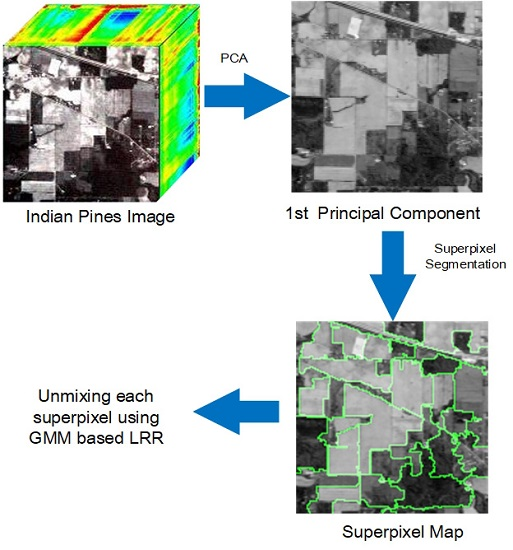
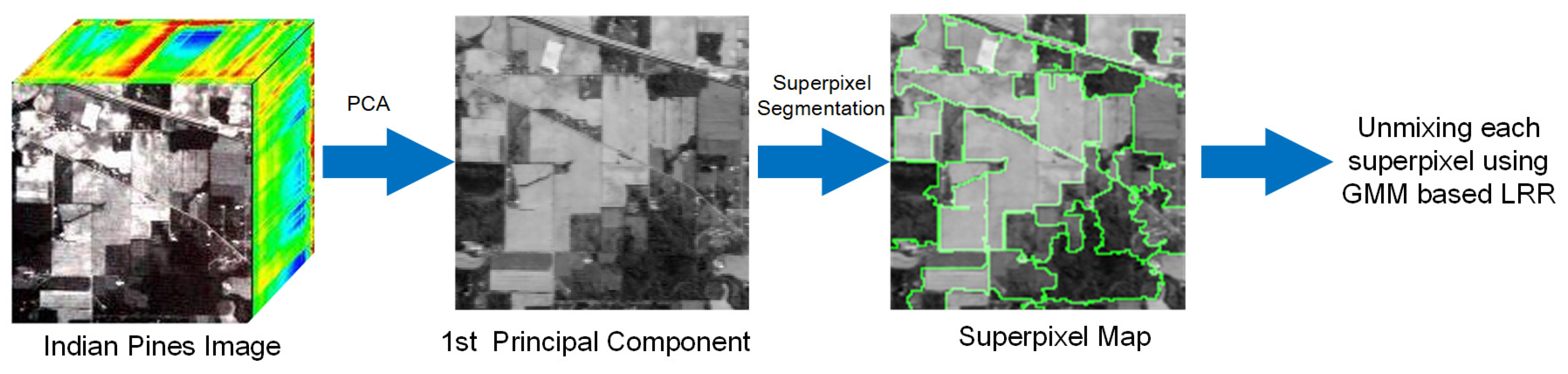
Input: Collect mixed pixel matrix $\mathbf{Y}$, endmember $\mathbf{E}$, the parameter of smoothness and sparse constraint ${\beta }_1,{\beta }_2$, and the parameter of low-rank property ${\beta }_3$ and the number of the superpixels S; Output: The estimated abundance matrix $\mathbf{A}$;  1: Implement PCA on $\mathbf{Y}$ and obtain the first principal component;  2: Segment $\mathbf{Y}$ into homogeneous regions based on its first principal component by using entropy rate [42];  3: for each homogeneous region do  4:  |Recover $\mathbf{A}$ with Algorithm 1;  5: end for  6: Obtain $\mathbf{A}$ from each homogeneous region;  7: Return $\mathbf{A}$.

4. Experimental Result

We evaluated the performances of the proposed GMM-SS-LRR and compared it with the state-of-the-art algorithms on synthetic datasets and real HSIs. To demonstrate the efficiency of the proposed GMM-SS-LRR, we mainly compared it with three other algorithms, namely the normal compositional model (NCM), the beta compositional model (BCM) (BCM takes the spectral version with quadratic programming) and GMM, because these three methods are both based on LMM and model the endmember using continuous distribution. For the proposed method GMM-SS-LRR and GMM, the original image data were projected to a subspace with 10 dimensions to speed up the computation for abundance estimation. Since NCM is a supervised algorithm, we took the ground truth pixels as input, and modeled them by an unimodal Gaussian distribution and obtained the abundance maps by maximizing the log-likelihood. BCM was also implemented as a supervised algorithm; ground truth pure pixels were again taken as input and the results were the abundance maps. In the following experiments, we implemented the algorithm in MATLAB^® and experiments were performed on a laptop with 2.6-GHz Intel Core CPU, 16-GB memory. All parameters of ${\beta }_1$ (smoothness prior constraint) and ${\beta }_2$ (sparse prior constraint) were set following the GMM method [34] (in the synthetic dataset, the parameters were set to ${\beta }_1=0.1,{\beta }_2=0.1$; and in the real HSIs, the parameters were set to ${\beta }_1=5,{\beta }_2=5$ ), and, for the proposed GMM-SS-LRR method, the low-rank property in the synthetic dataset was set to ${\beta }_3=0.1$ and in the real HSIs was set to ${\beta }_3=1$. The number of superpixels for both synthetic dataset and real HSIs was set to $\mathrm{S}=5$.

For comparison of abundances, we calculated the root mean squared error (RMSE) for abundance error, which is defined as follows:

$$\mathrm{RMSE}=(\frac{1}{N}\sum _n|{\alpha }_{nj}^{GT}-{\alpha }_{nj}^{est}{{|}^2)}^{1/2},$$

(29)

where ${\alpha }_{nj}^{GT}$ are the ground truth abundances and ${\alpha }_{nj}^{est}$ are the estimated values. Since only some pure pixels were identified as ground truth in the real HSI dataset, we calculated ${\mathrm{error}}_j=(\frac{1}{\left|\mathcal{I}\right|}{\sum }_{n\in \mathcal{I}}|{\alpha }_{nj}^{GT}-{\alpha }_{nj}^{est}{{|}^2)}^{1/2}$ given the pure pixel index set $\mathcal{I}$.

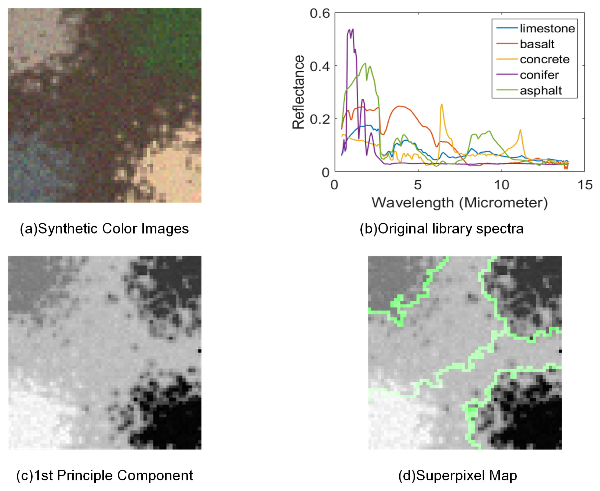
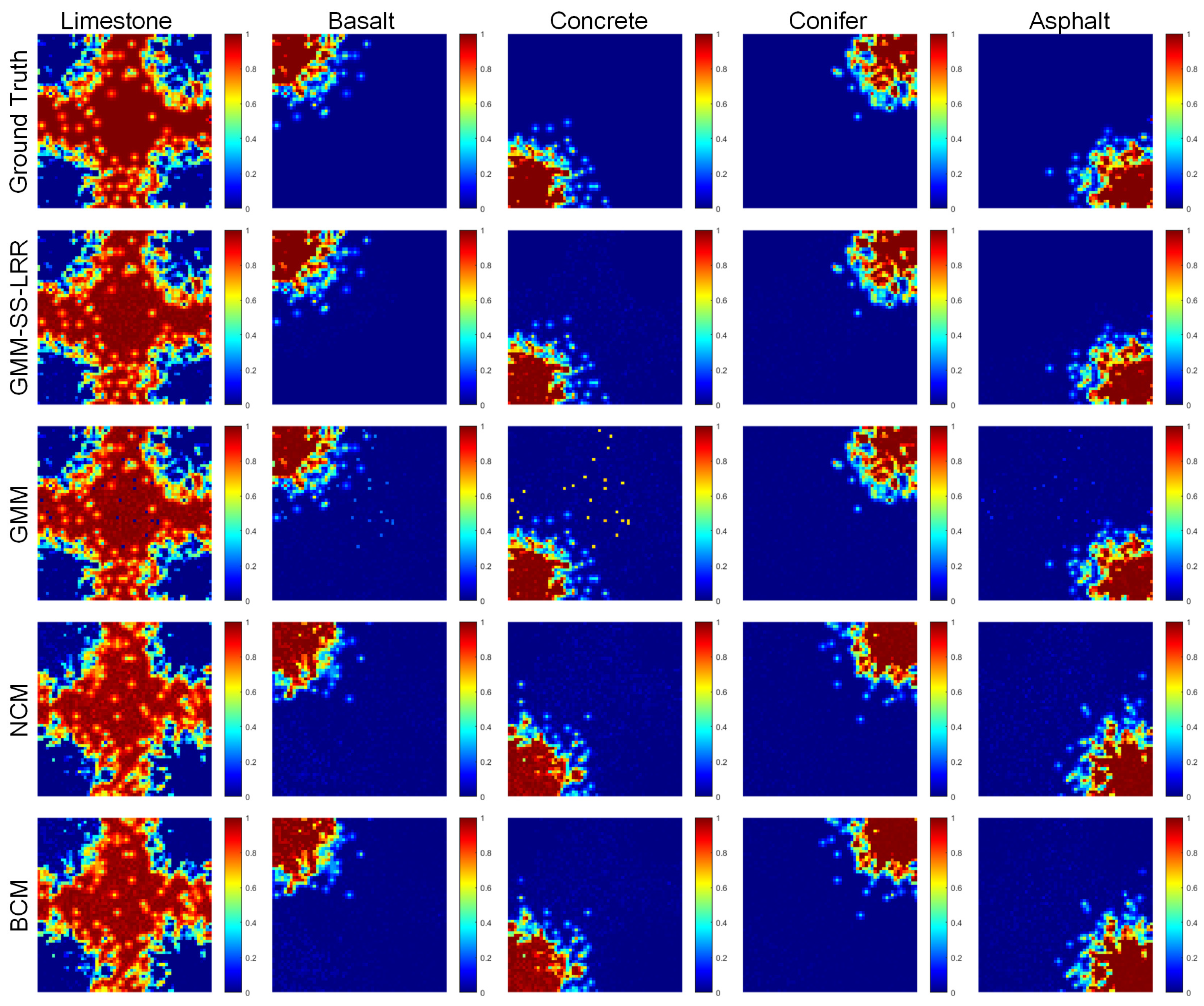
4.1. Synthetic Datasets

For the synthetic data experiments, the mean endmember spectra we used were randomly selected from the ASTER spectral library [24] with slight constant changes (their original spectra are shown in Figure 2b), which determined a spectral range from 0.4 μm to 14 μm. The size of the synthetic was $60\times 60$ pixels and constructed from five endmembers (limestone, basalt, concrete, conifer and asphalt), whose spectral signatures are highly differentiable. The covariance matrices Were constructed by ${\alpha }_{jk}^2{\mathbf{I}}_B+b_{jk}^2{\mathit{\mu }}_{jk}{\mathit{\mu }}_{jk}^T$ where ${\mathit{\mu }}_{jk}$ is a unit vector controlling the major variation direction. We made the first material as background, and the procedure of generating the abundance maps followed Zhou et al. [52]: for each other material (not as background), 600 Gaussian blobs were randomly placed in the corner, and the shape, width and location were sampled from Gaussian distributions. The Gaussian noise was added to generated pixels; the noise sigma was set with ${\sigma }_Y=0.001$. Figure 2a shows the resulting color images by extracting the bands corresponding to wavelengths 488 nm, 556 nm, and 693 nm. The endmember spectra we used to generate the synthetic data are shown in Figure 3, where we can see the centers and the major variations of the Gaussians.

Figure 2c,d shows the first principle component of the synthetic dataset and the superpixel map we used, respectively. The synthetic image was correctly partitioned into several regions, whose shape and size were accustomed on the basis of different spatial structures, meaning there was a high degree of correlation among the spectral signatures of the neighboring pixels, hence we could take low-rank representation to further exploit the spatial information and improve the abundance estimation. The abundance maps of our method and other comparison algorithms for the synthetic dataset are shown in Figure 4; since the materials were randomly placed in the corner, the abundance maps of the last four materials (basalt, concrete, conifer and asphalt) look relatively clean and less cluttered. Comparing them with the ground truth, we can see that all algorithms correctly estimated the abundance maps scatter. However, for BCM and NCM, although the abundance maps performed relatively clean as well, the shape and size were quite different compared with the ground truth. This means that many pixels with original abundance of 1 were predicted to have abundance of 0, which caused a relatively large value of RMSE. As for the GMM method, although the abundance maps appeared to have clutter point, the shape and size were similar to the ground truth. Hence, the estimating accuracy was higher than NCM and BCM. The GMM-SS-LRR algorithm with SS and low-rank property was much closer to the ground truth map. The quantitative analysis of those four algorithms is shown in

Table 1. Abundance errors for synthetic dataset.

$\times {10}^{-4}$	GMM-SS-LRR	GMM	NCM	BCM
Limestone	142	816	566	743
Basalt	59	182	278	311
Concrete	94	539	460	586
Conifer	50	50	248	273
Asphalt	45	123	262	277
Whole map	78	342	363	438

.

The histograms of the synthetic pure pixels for the five materials are shown in Figure 5. Since the BCM algorithm was not modeled as Gaussian distribution, the probability of each distribution was only compared among GMM-SS-LRR, GMM and NCM algorithm. The histogram was the statistical probability value of the pure materials for the five materials (when projected to one-dimensional space determined by performing PCA). The probability of each distribution was calculated by multiplying the value of the density function at each bin location with the bin size. Figure 5 shows that the graph of NCM is similar to GMM and GMM-SS-LRR when the distribution of pure pixels was generated by an unimodal Gaussian. Nevertheless, for basalt and concrete, GMM and GMM-SS-LRR provided a more accurate estimation because NCM was modeled by a single Gaussian hypothesis. When comparing GMM and GMM-SS-LRR, the distribution was similar for limestone, concrete, conifer and asphalt. However, for basalt, GMM-SS-LRR fitted the histograms better than GMM, as the first step in GMM approach was to separate the library into several groups, each of which representing a material and clustered into several centers. The size of each cluster affected the probability of picking its center to a large extent. When directly using the GMM method for unmixing, sometimes the estimated distribution of the cluster did not fit the ground truth well. Taking SS in the first principle component of HSI helped the GMM better separate the clusters. The quantitative analysis of these three algorithms is shown in

Table 2. The RMSE calculated between the probability value in each histogram and the estimated value at each bin location for the synthetic dataset.

$\times {10}^{-4}$	GMM-SS-LRR	GMM	NCM
Limestone	60	62	81
Basalt	89	134	248
Concrete	90	93	259
Conifer	72	72	160
Asphalt	94	94	140

. We calculated the probability value in each histograms between the ground truth and estimate value using Equation (29).

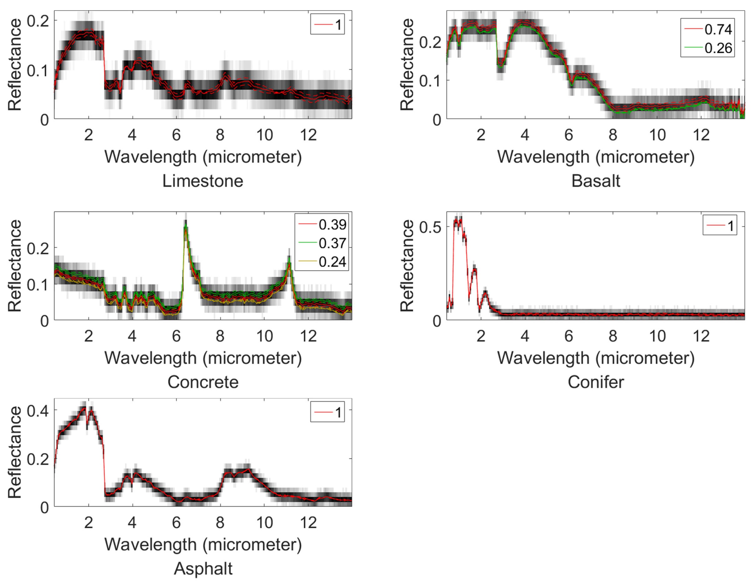
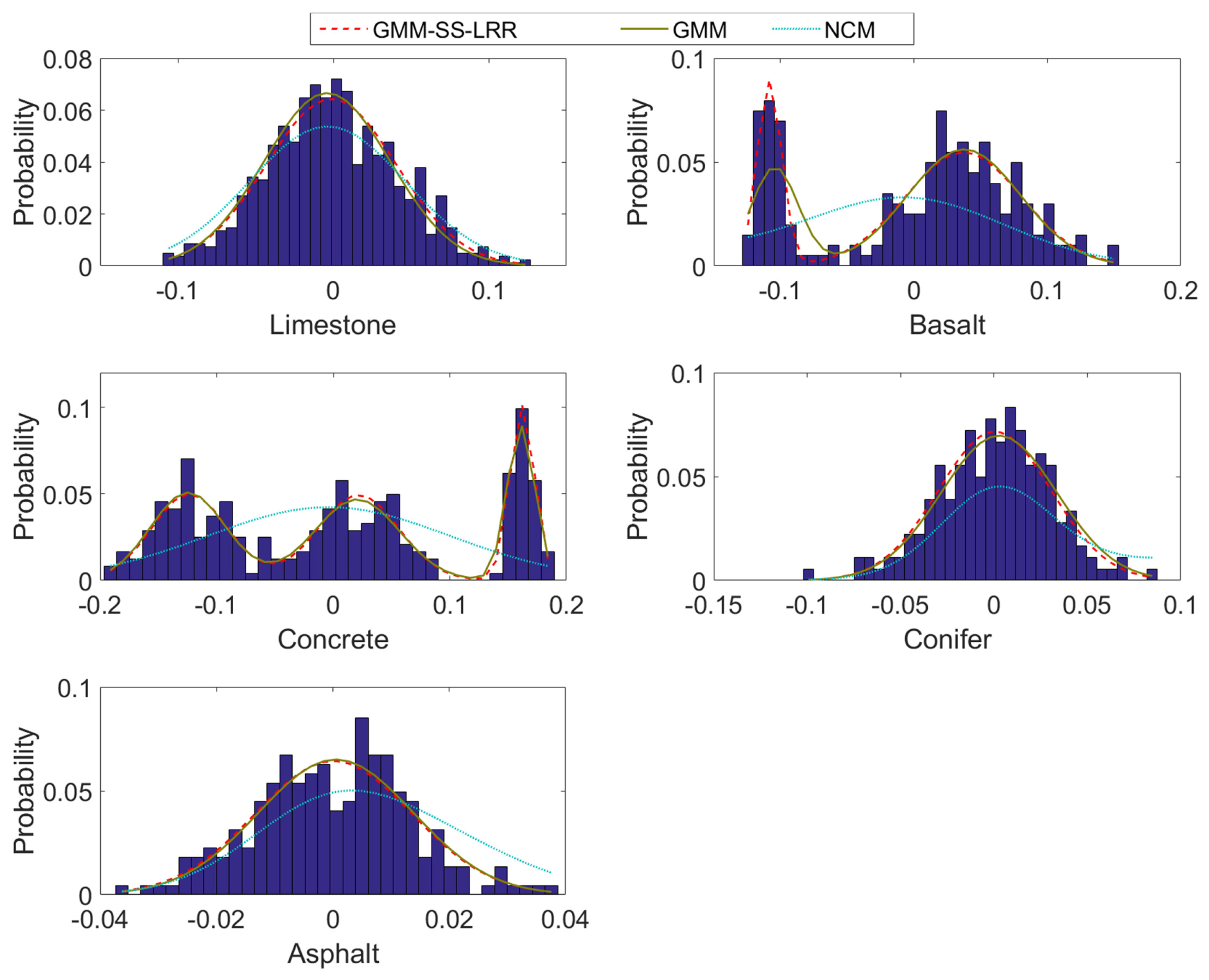
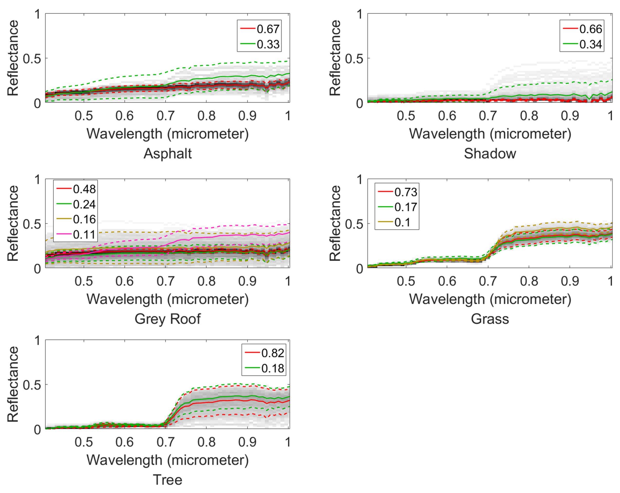
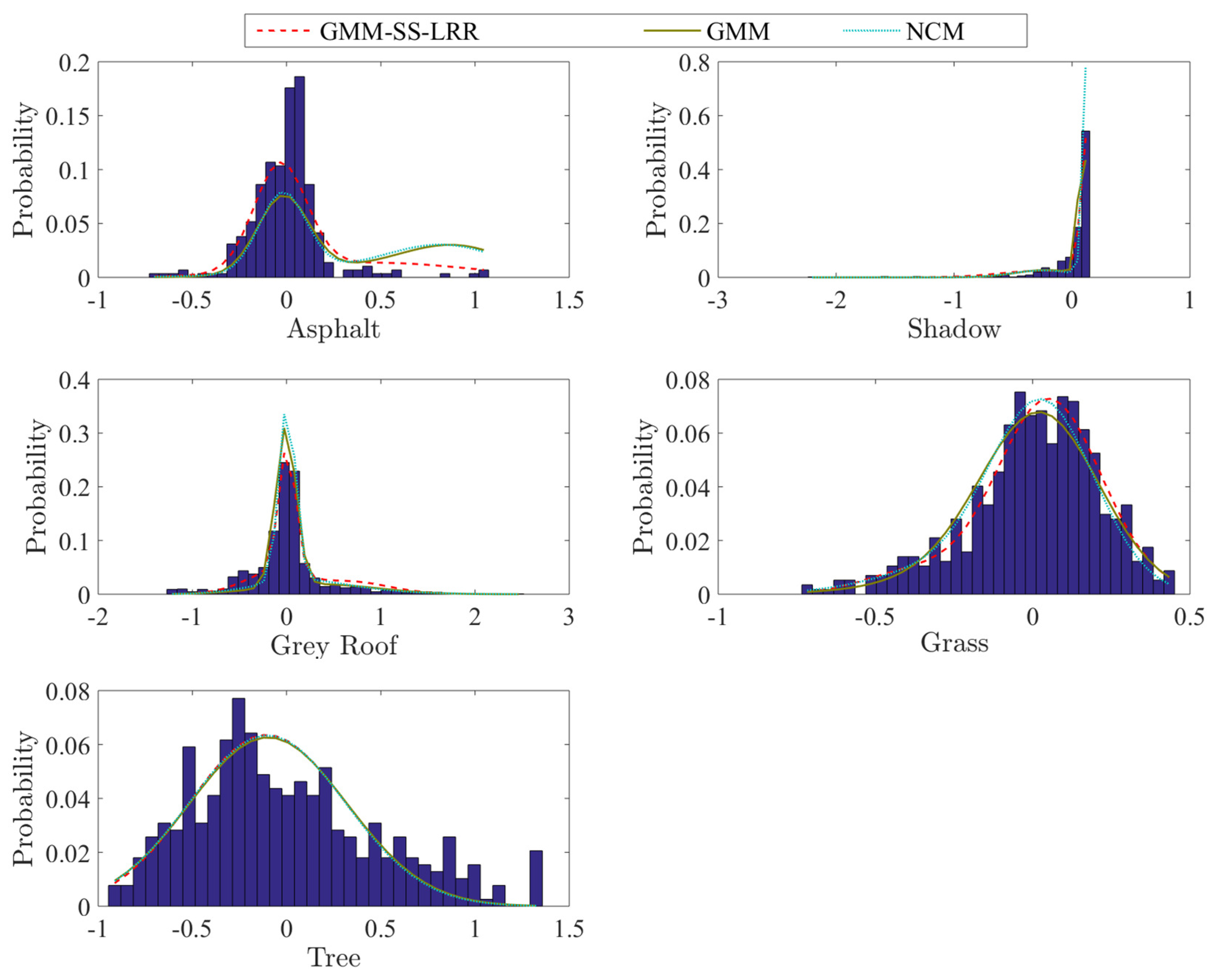
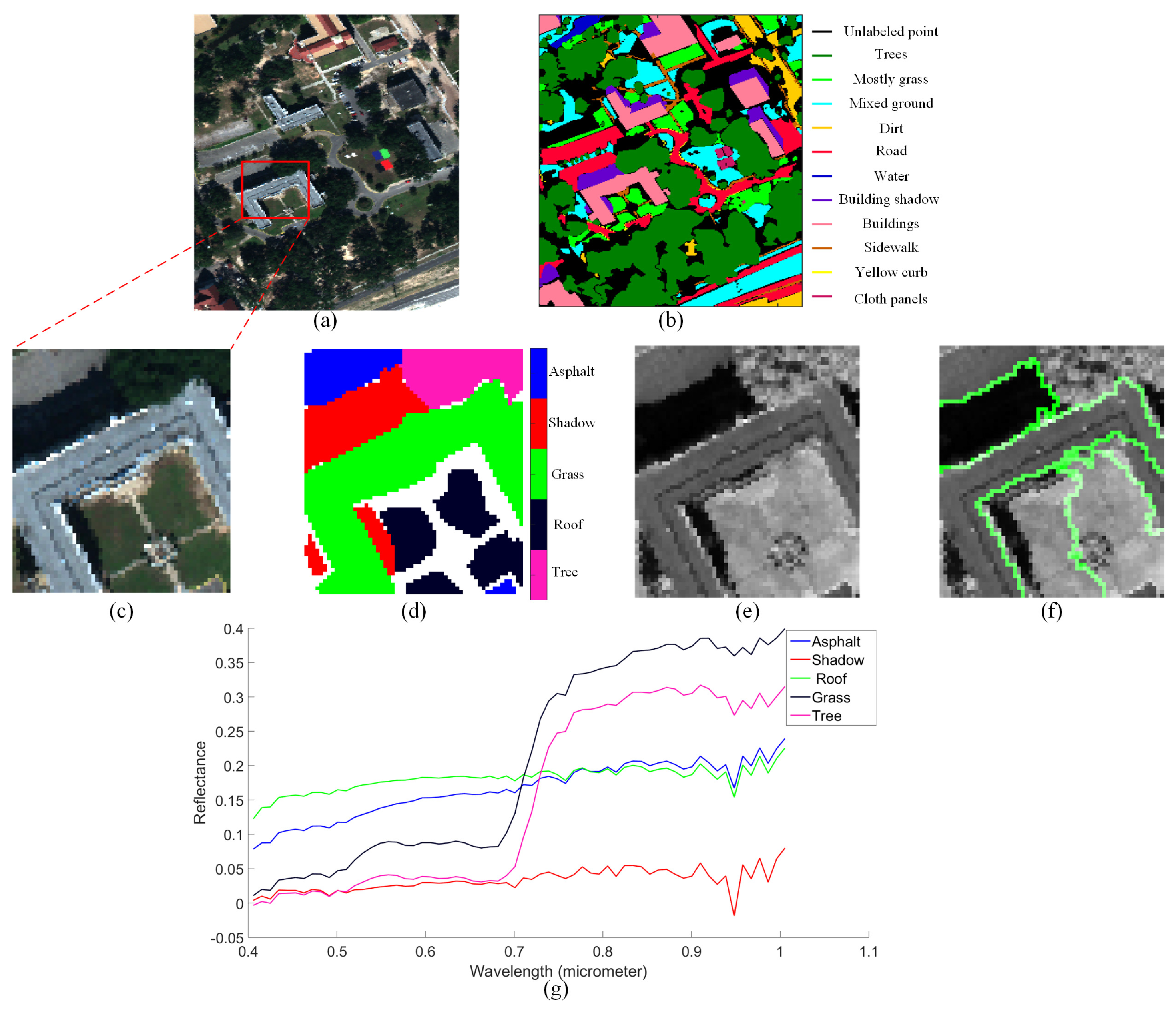
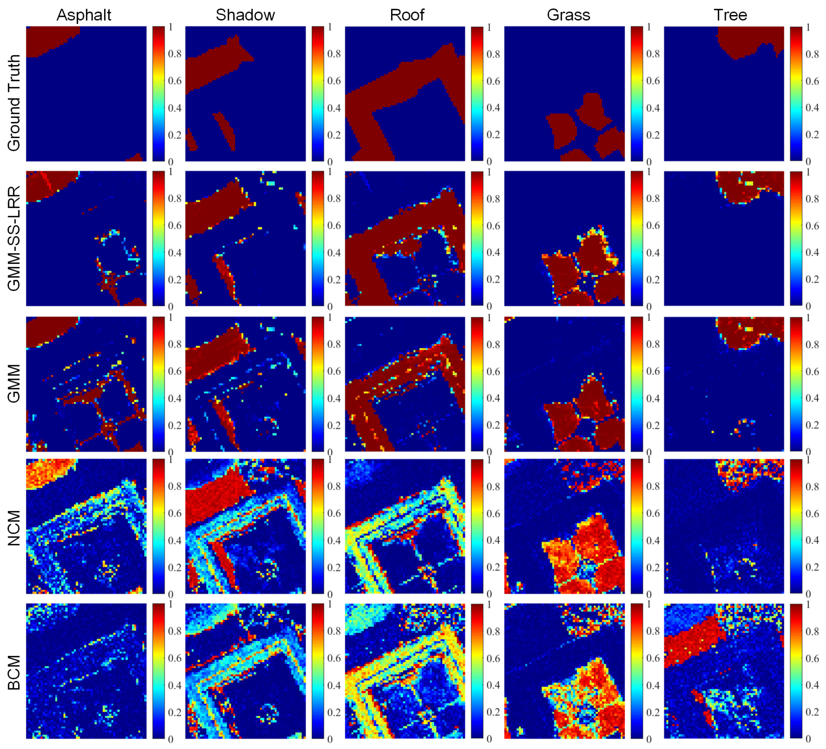
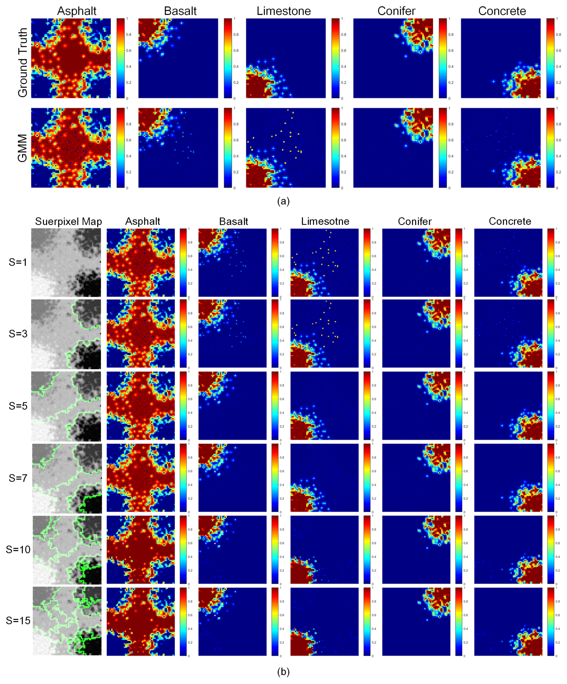
4.2. Mississippi Gulfport Datasets

The dataset was collected at the University of Southern Mississippi’s Gulfpark Campus, and is a 289 × 284 image with 72 bands corresponding to wavelengths from 0.368 μm to 1.043 μm. The spatial resolution is 1 m/pixel. The scene contains several man-made and natural materials including sidewalks, roads, various types of building roofs, concretes, shrubs, trees and grasses. To better compare the performance between our method and GMM, we chose the same ROI area followed in [34]. The ROI was a 58 by 65 pixel area containing five materials. The original RGB image and the selected ROI are shown in Figure 6a,c.

Figure 7 shows the abundance maps comparison in the Gulfport dataset. Comparing them with the ground truth (the first row of Figure 7), we can see that BCM failed to estimate the pure pixels of tree, even though ground truth pure pixels were used for training. For example, the fourth and fifth abundance maps of BCM showed that the pixels of tree were mixed with grass and asphalt. For BCM and NCM, we did not use PCA to get the main information while using the original HSI dataset as input. However, they still performed poorly on this dataset. The result of GMM-SS-LRR not only showed sparse abundances for the region but also interpreted the boundary as a combination of neighboring materials. Although the results of GMM method appeared to be good in general, the abundances in a pure material region were inconsistent. The result of these abundance maps also verified that the GMM-SS-LRR algorithm with SS and low-rank property could better capture the spatial data structure and enhance the performance in the abundance estimation. The errors of abundances for these algorithms are shown in

Table 3. Abundance errors for Gulfport dataset.

$\times {10}^{-3}$	GMM-SS-LRR	GMM	NCM	BCM
Asphalt	161	202	383	865
Shadow	136	149	151	888
Roof	216	338	627	536
Grass	10	21	166	341
Tree	197	183	647	761
Whole map	99	140	278	328

, which demonstrates that GMM-SS-LRR performed best overall.

Figure 8 shows the GMM-SS-LRR result in the wavelength–reflectance space for the Gulfport. Figure 9 shows histograms of pure pixels for the five materials (when projected to one-dimensional space determined by performing PCA on the pure pixels of each material) of the Gulfport dataset. Although there were no multiple peaks in any of the histograms, NCM algorithm still did not fit the histograms of the shadow. In contrast, our method and GMM algorithm gave a much better fit for this pure pixel distribution. For the performance of all five materials, our method matched the ground truth best, and this was also verified in the quantitative analysis presented in

Table 4. The RMSE calculated between the probability value in each histogram and the estimated value at each bin location for the Gulfport dataset.

$\times {10}^{-3}$	GMM-SS-LRR	GMM	NCM
Asphalt	229	322	332
Shadow	137	273	473
Roof	91	163	186
Grass	81	88	70
Tree	110	110	111

.

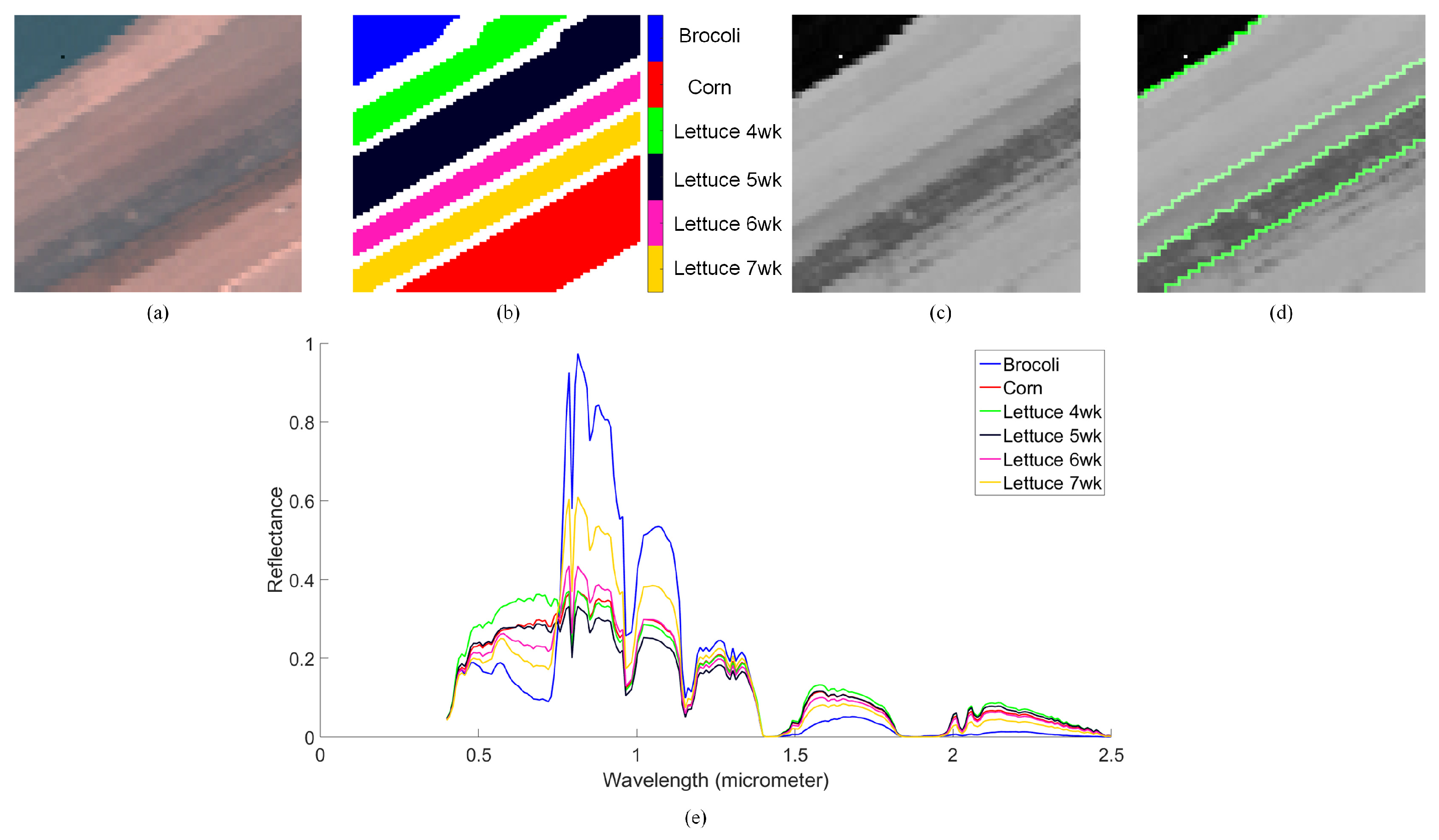
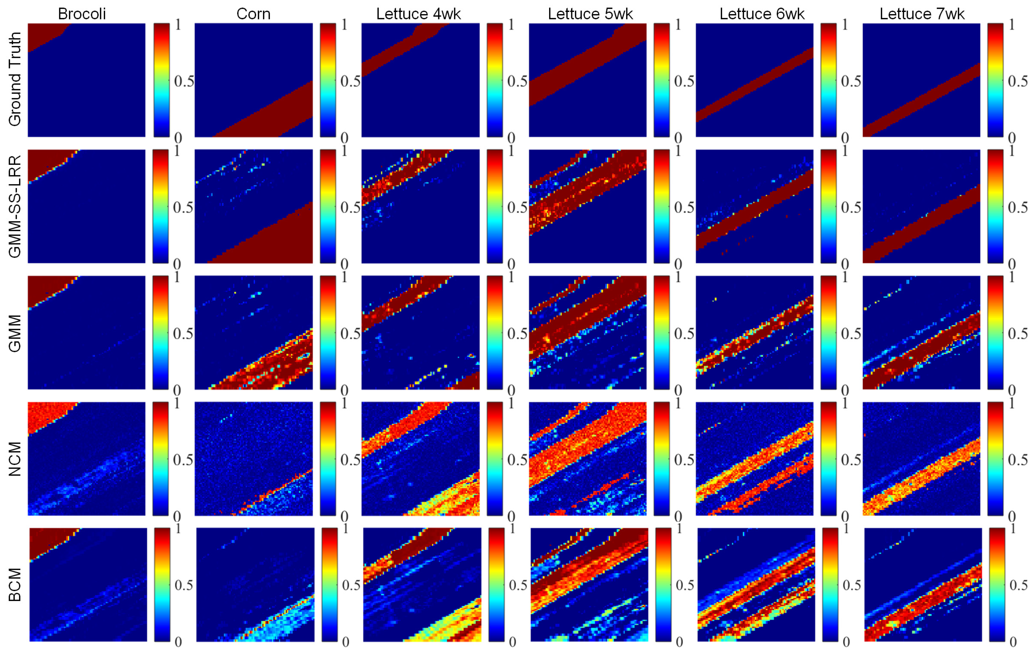
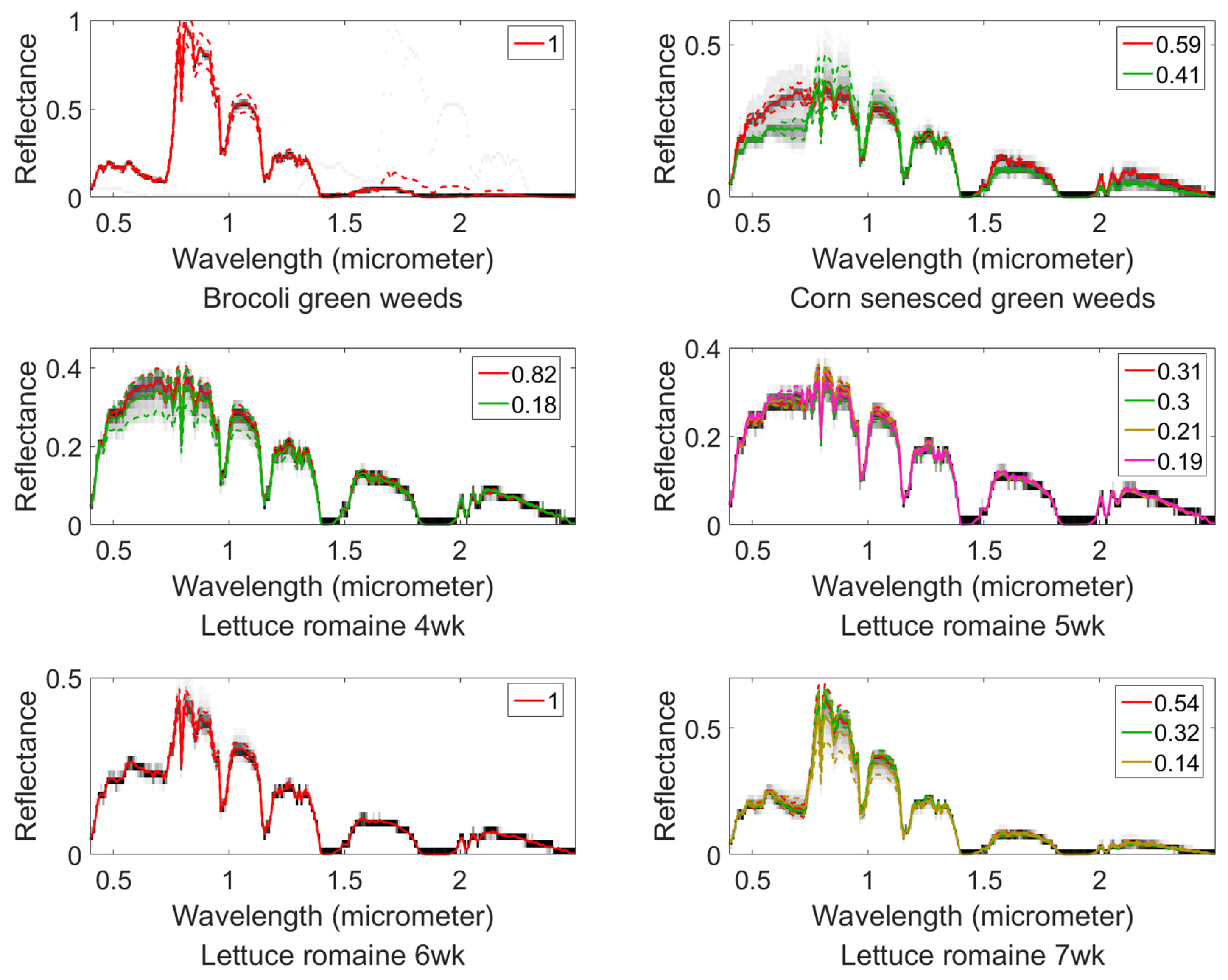
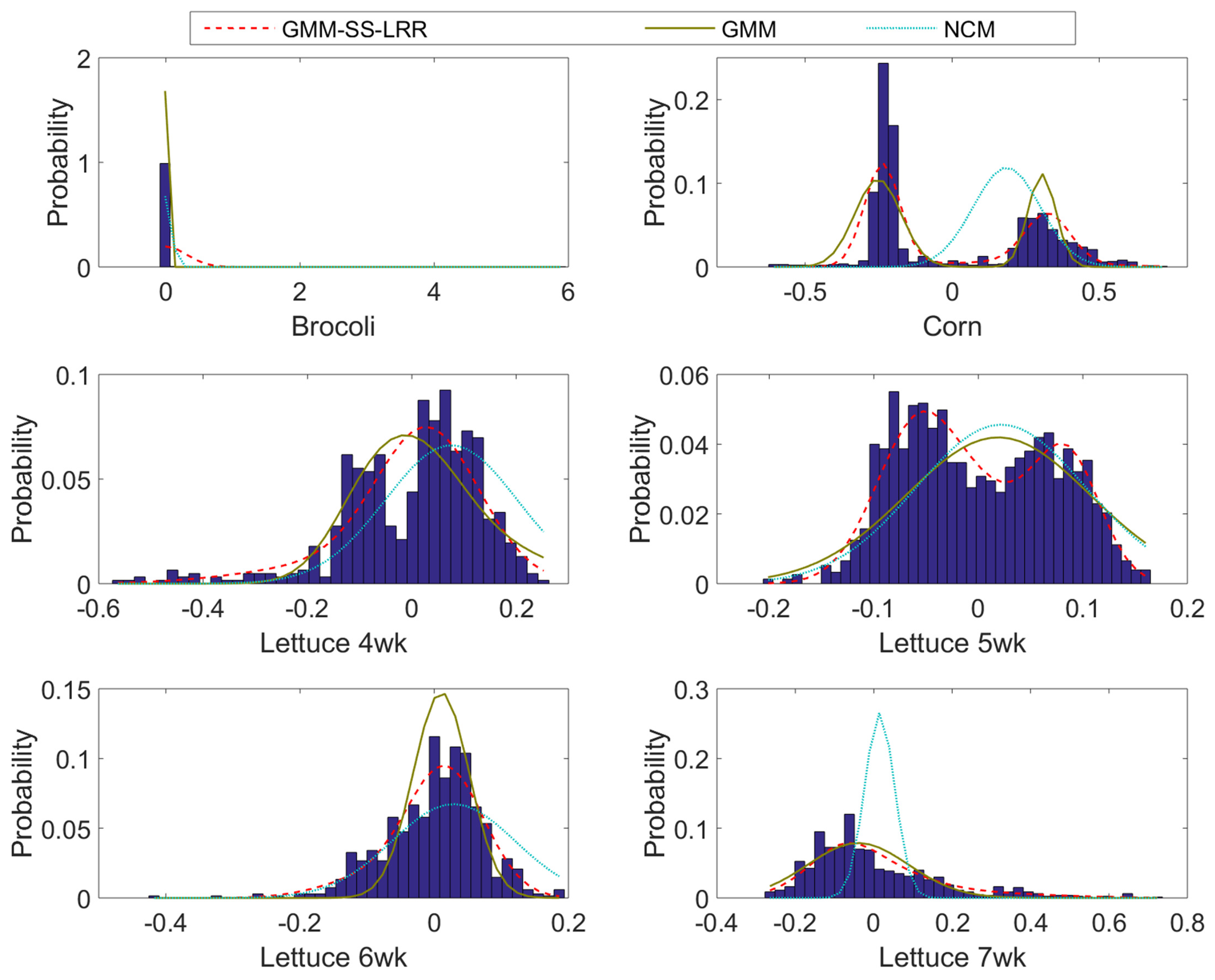
4.3. Salinas-A Datasets

The dataset was collected by the AVIRIS sensor over Salinas Valley, California, and is characterized by high spatial resolution (3.7-m pixels). It is a 512 by 217 image with 224 bands. The original image includes vegetables, bare soils, and vineyard fields. Considering that the whole dataset contains many different objects, we only performed experiments on the exemplar ROI. It is a small sub scene of Salinas image, denoted Salinas-A, which is commonly used. It comprises 86 by 83 pixels and includes six classes: broccoli, corn, lettuce 4wk, lettuce 5wk, lettuce 6wk and lettuce 7wk. The RGB image, ground truth and the superpixel map are shown in Figure 10.

Figure 11 shows the abundance maps comparison in the Salinas-A dataset. Comparing them with the ground truth (the first row of Figure 11), we can see that BCM and NCM both failed to estimate the pure pixels of corn, and, as for the lettuce 4wk, the abundance maps of GMM, NCM and BCM were mixed with the endmember corn. GMM-SS-LRR matched the ground truth best followed by GMM. The errors of abundances for these algorithms are shown in

Table 5. Abundance errors for Sainas-A dataset.

$\times {10}^{-3}$	GMM-SS-LRR	GMM	NCM	BCM
Brocoli	506	715	1421	511
Corn	386	2087	8790	8021
Lettuce 4wk	2090	2096	2732	2396
Lettuce 5wk	710	520	1858	1536
Lettuce 6wk	551	1975	2529	1597
Lettuce 7wk	1061	1046	3053	2423
Whole map	498	802	2268	2006

, which also implies that GMM-SS-LRR performed best overall. Figure 12 shows GMM-SS-LRR result in the wavelength–reflectance space. Figure 13 shows histograms of pure pixels for the six materials and the estimated distributions of GMM-SS-LRR, GMM and NCM. When the distribution of pure pixels was a single peak, the NCM algorithm still did not closely approximate the ground truth. In the lettuce 5wk, the GMM algorithm failed to estimate the distribution since the pure pixels had multiple peaks. This also showed that our method helped the GMM better separate the clusters and improve the performance in the estimated distribution. The quantitative analysis is shown in

Table 6. The RMSE calculated between the probability value in each histogram and the estimated value at each bin location for the Sainas-A dataset.

$\times {10}^{-4}$	GMM-SS-LRR	GMM	NCM
Brocoli	1303	1196	552
Corn	264	342	607
Lettuce 4wk	140	159	164
Lettuce 5wk	51	112	120
Lettuce 6wk	122	187	138
Lettuce 7wk	110	133	599

.

4.4. Effects of the Size of the Superpixels

For the proposed method GMM-SS-LRR, the number of superpixels for both synthetic dataset and real HSIs was set to $\mathrm{S}=5$. To compare the effects of different sizes of superpixels on the unmixing accuracy, we experimented with the synthetic dataset by changing the size of the parameters S. From the first row of Figure 14b, we can see that, when $\mathrm{S}=1$, the GMM-SS-LRR abundance maps were similar to those of GMM (the second row of Figure 14a), which means that, when we did not take the SS, the pixels were not in the homogeneous region, thus only taking low-rank representation for prior constraint could not improve the performance of the abundance estimation. As the number S increased, the performance of the abundance estimation was improved. Compared with the ground truth (the first row of Figure 14a), we can see that, when the number of superpixels S was set to 5 and 7, the precision of unmixing became the best. That means only segmenting the pixel into a highly spatially related region, and then taking low-rank representation could greatly improve the abundance estimation. However, when the number of superpixels S was set to 10 and 15, the accuracy of the unmixing declined. This was because, when the superpixel was too small, there were not enough data for training, and those superpixels had no statistical significance. The quantitative analysis of different size of superpixels is shown in

Table 7. GMM-SS-LRR abundance errors with different sizes of superpixels for synthetic dataset.

GMM-SS-LRR	S = 1	S = 3	S = 5	S = 7	S = 10	S = 15
Limestone	816	813	142	142	628	645
Basalt	182	180	59	58	168	170
Concrete	539	537	93	93	491	508
Conifer	50	47	50	48	96	96
Asphalt	123	120	45	46	182	186
Whole map	342	339	78	77	313	321

.

5. Conclusions

In this paper, we propose a GMM-SS-LRR method for hyperspectral abundances estimation problem based on the GMM, which can achieve better abundance estimation results and fully consider the possible spatial correlation between local pixels. Taking SS in the first principal component of HSI to get the homogeneous regions can help the GMM method make pixels and their associated abundances similar for the adjacent pixels, and enhance the performance of the endmember estimation. Using low-rank property in the homogeneous regions can also get better abundance estimation. Moreover, considering the endmember variability phenomenon, under the Bayesian framework, we use GMM to formulate the unmixing problem, and put the low-rank property into the objective function as a prior knowledge; the conditional density function leads to a MAP problem that can be solved by the GEM method. The experiments on both synthetic datasets and real HSI demonstrated that the proposed GMM-SS-LRR is efficient for solving the hyperspectral unmixing problem compared with the other algorithms such as GMM, NCM, and BCM.

References

1. Bioucas-Dias, J.M.; Plaza, A.; Dobigeon, N.; Parente, M.; Du, Q.; Gader, P.; Chanussot, J. Hyperspectral unmixing overview: Geometrical, statistical, and sparse regression-based approaches. IEEE J. Sel. Top. Appl. Earth Obs. Remote Sens. 2012, 5, 354–379. [Google Scholar] [CrossRef]
2. Mei, X.; Ma, Y.; Li, C.; Fan, F.; Huang, J.; Ma, J. Robust GBM hyperspectral image unmixing with superpixel segmentation based low rank and sparse representation. Neurocomputing 2018, 275, 2783–2797. [Google Scholar] [CrossRef]
3. Jiang, J.; Ma, J.; Wang, Z.; Chen, C.; Liu, X. Hyperspectral Image Classification in the Presence of Noisy Labels. IEEE Trans. Geosci. Remote Sens. 2019, 57, 851–865. [Google Scholar] [CrossRef]
4. Ma, J.; Zhou, H.; Zhao, J.; Gao, Y.; Jiang, J.; Tian, J. Robust feature matching for remote sensing image registration via locally linear transforming. IEEE Trans. Geosci. Remote Sens. 2015, 53, 6469–6481. [Google Scholar] [CrossRef]
5. Manolakis, D.; Siracusa, C.; Shaw, G. Hyperspectral subpixel target detection using the linear mixing model. IEEE Trans. Geosci. Remote Sens. 2001, 39, 1392–1409. [Google Scholar] [CrossRef]
6. Ma, L.; Crawford, M.M.; Zhu, L.; Liu, Y. Centroid and Covariance Alignment-Based Domain Adaptation for Unsupervised Classification of Remote Sensing Images. IEEE Trans. Geosci. Remote Sens. 2019, 57, 2305–2323. [Google Scholar] [CrossRef]
7. Jiang, J.; Ma, J.; Chen, C.; Wang, Z.; Cai, Z.; Wang, L. SuperPCA: A Superpixelwise PCA Approach for Unsupervised Feature Extraction of Hyperspectral Imagery. IEEE Trans. Geosci. Remote Sens. 2018, 56, 4581–4593. [Google Scholar] [CrossRef]
8. Ma, J.; Zhao, J.; Jiang, J.; Zhou, H.; Guo, X. Locality preserving matching. Int. J. Comput. Vis. 2019, 127, 512–531. [Google Scholar] [CrossRef]
9. Ghamisi, P.; Yokoya, N.; Li, J.; Liao, W.; Liu, S.; Plaza, J.; Rasti, B.; Plaza, A. Advances in hyperspectral image and signal processing: A comprehensive overview of the state of the art. IEEE Geosci. Remote Sens. Mag. 2017, 5, 37–78. [Google Scholar] [CrossRef]
10. Boardman, J.W.; Kruse, F.A.; Green, R.O. Mapping Target Signatures via Partial Unmixing of AVIRIS Data. 1995. Available online: http://hdl.handle.net/2014/33635 (accessed on 14 April 2019).
11. Ren, H.; Chang, C.I. Automatic spectral target recognition in hyperspectral imagery. IEEE Trans. Aerosp. Electron. Syst. 2003, 39, 1232–1249. [Google Scholar]
12. Nascimento, J.M.; Dias, J.M. Vertex component analysis: A fast algorithm to unmix hyperspectral data. IEEE Trans. Geosci. Remote Sens. 2005, 43, 898–910. [Google Scholar] [CrossRef]
13. Chan, T.H.; Ma, W.K.; Ambikapathi, A.; Chi, C.Y. A simplex volume maximization framework for hyperspectral endmember extraction. IEEE Trans. Geosci. Remote Sens. 2011, 49, 4177–4193. [Google Scholar] [CrossRef]
14. Berman, M.; Kiiveri, H.; Lagerstrom, R.; Ernst, A.; Dunne, R.; Huntington, J.F. ICE: A statistical approach to identifying endmembers in hyperspectral images. IEEE Trans. Geosci. Remote Sens. 2004, 42, 2085–2095. [Google Scholar] [CrossRef]
15. Halimi, A.; Altmann, Y.; Dobigeon, N.; Tourneret, J.Y. Nonlinear unmixing of hyperspectral images using a generalized bilinear model. IEEE Trans. Geosci. Remote Sens. 2011, 49, 4153–4162. [Google Scholar] [CrossRef]
16. Altmann, Y.; Halimi, A.; Dobigeon, N.; Tourneret, J.Y. Supervised nonlinear spectral unmixing using a postnonlinear mixing model for hyperspectral imagery. IEEE Trans. Image Process. 2012, 21, 3017–3025. [Google Scholar] [CrossRef]
17. Broadwater, J.; Chellappa, R.; Banerjee, A.; Burlina, P. Kernel fully constrained least squares abundance estimates. In Proceedings of the 2007 IEEE International Geoscience and Remote Sensing Symposium, Barcelona, Spain, 23–28 July 2007; pp. 4041–4044. [Google Scholar]
18. Broadwater, J.; Banerjee, A. A generalized kernel for areal and intimate mixtures. In Proceedings of the 2010 2nd Workshop on Hyperspectral Image and Signal Processing: Evolution in Remote Sensing (WHISPERS), Reykjavik, Iceland, 14–16 June 2010; pp. 1–4. [Google Scholar]
19. Heylen, R.; Parente, M.; Gader, P. A review of nonlinear hyperspectral unmixing methods. IEEE J. Sel. Top. Appl. Earth Obs. Remote Sens. 2014, 7, 1844–1868. [Google Scholar] [CrossRef]
20. Zare, A.; Ho, K. Endmember variability in hyperspectral analysis: Addressing spectral variability during spectral unmixing. IEEE Signal Process. Mag. 2014, 31, 95–104. [Google Scholar] [CrossRef]
21. Roberts, D.A.; Gardner, M.; Church, R.; Ustin, S.; Scheer, G.; Green, R. Mapping chaparral in the Santa Monica Mountains using multiple endmember spectral mixture models. Remote Sens. Environ. 1998, 65, 267–279. [Google Scholar] [CrossRef]
22. Combe, J.P.; Le Mouélic, S.; Sotin, C.; Gendrin, A.; Mustard, J.; Le Deit, L.; Launeau, P.; Bibring, J.P.; Gondet, B.; Langevin, Y.; et al. Analysis of OMEGA/Mars express data hyperspectral data using a multiple-endmember linear spectral unmixing model (MELSUM): Methodology and first results. Planet. Space Sci. 2008, 56, 951–975. [Google Scholar] [CrossRef]
23. Asner, G.P.; Lobell, D.B. A biogeophysical approach for automated SWIR unmixing of soils and vegetation. Remote Sens. Environ. 2000, 74, 99–112. [Google Scholar] [CrossRef]
24. Asner, G.P.; Heidebrecht, K.B. Spectral unmixing of vegetation, soil and dry carbon cover in arid regions: Comparing multispectral and hyperspectral observations. Int. J. Remote Sens. 2002, 23, 3939–3958. [Google Scholar] [CrossRef]
25. Dennison, P.E.; Roberts, D.A. Endmember selection for multiple endmember spectral mixture analysis using endmember average RMSE. Remote Sens. Environ. 2003, 87, 123–135. [Google Scholar] [CrossRef]
26. Bateson, C.A.; Asner, G.P.; Wessman, C.A. Endmember bundles: A new approach to incorporating endmember variability into spectral mixture analysis. IEEE Trans. Geosci. Remote Sens. 2000, 38, 1083–1094. [Google Scholar] [CrossRef]
27. Somers, B.; Asner, G.P.; Tits, L.; Coppin, P. Endmember variability in spectral mixture analysis: A review. Remote Sens. Environ. 2011, 115, 1603–1616. [Google Scholar]
28. Jin, J.; Wang, B.; Zhang, L. A novel approach based on fisher discriminant null space for decomposition of mixed pixels in hyperspectral imagery. IEEE Geosci. Remote Sens. Lett. 2010, 7, 699–703. [Google Scholar] [CrossRef]
29. Eches, O.; Dobigeon, N.; Mailhes, C.; Tourneret, J.Y. Bayesian estimation of linear mixtures using the normal compositional model. Application to hyperspectral imagery. IEEE Trans. Image Process. 2010, 19, 1403–1413. [Google Scholar] [CrossRef]
30. Stein, D. Application of the normal compositional model to the analysis of hyperspectral imagery. In Proceedings of the 2003 IEEE Workshop on Advances in Techniques for Analysis of Remotely Sensed Data, Greenbelt, MD, USA, 27–28 October 2003; pp. 44–51. [Google Scholar]
31. Halimi, A.; Dobigeon, N.; Tourneret, J.Y. Unsupervised unmixing of hyperspectral images accounting for endmember variability. IEEE Trans. Image Process. 2015, 24, 4904–4917. [Google Scholar] [CrossRef]
32. Zhang, B.; Zhuang, L.; Gao, L.; Luo, W.; Ran, Q.; Du, Q. PSO-EM: A hyperspectral unmixing algorithm based on normal compositional model. IEEE Trans. Geosci. Remote Sens. 2014, 52, 7782–7792. [Google Scholar] [CrossRef]
33. Du, X.; Zare, A.; Gader, P.; Dranishnikov, D. Spatial and spectral unmixing using the beta compositional model. IEEE J. Sel. Top. Appl. Earth Obs. Remote Sens. 2014, 7, 1994–2003. [Google Scholar]
34. Zhou, Y.; Rangarajan, A.; Gader, P.D. A Gaussian mixture model representation of endmember variability in hyperspectral unmixing. IEEE Trans. Image Process. 2018, 27, 2242–2256. [Google Scholar] [CrossRef]
35. Eches, O.; Dobigeon, N.; Tourneret, J.Y. Enhancing hyperspectral image unmixing with spatial correlations. IEEE Trans. Geosci. Remote Sens. 2011, 49, 4239. [Google Scholar] [CrossRef]
36. Giampouras, P.V.; Themelis, K.E.; Rontogiannis, A.A.; Koutroumbas, K.D. Simultaneously sparse and low-rank abundance matrix estimation for hyperspectral image unmixing. IEEE Trans. Geosci. Remote Sens. 2016, 54, 4775–4789. [Google Scholar] [CrossRef]
37. Dobigeon, N.; Tourneret, J.Y.; Chang, C.I. Semi-supervised linear spectral unmixing using a hierarchical Bayesian model for hyperspectral imagery. IEEE Trans. Signal Process. 2008, 56, 2684–2695. [Google Scholar] [CrossRef]
38. Dobigeon, N.; Moussaoui, S.; Coulon, M.; Tourneret, J.Y.; Hero, A.O. Joint Bayesian endmember extraction and linear unmixing for hyperspectral imagery. IEEE Trans. Signal Process. 2009, 57, 4355–4368. [Google Scholar] [CrossRef]
39. Iordache, M.D.; Bioucas-Dias, J.M.; Plaza, A. Total variation spatial regularization for sparse hyperspectral unmixing. IEEE Trans. Geosci. Remote Sens. 2012, 50, 4484–4502. [Google Scholar] [CrossRef]
40. Qu, Q.; Nasrabadi, N.M.; Tran, T.D. Abundance estimation for bilinear mixture models via joint sparse and low-rank representation. IEEE Trans. Geosci. Remote Sens. 2014, 52, 4404–4423. [Google Scholar]
41. Meng, X.L.; Rubin, D.B. Maximum likelihood estimation via the ECM algorithm: A general framework. Biometrika 1993, 80, 267–278. [Google Scholar] [CrossRef]
42. Liu, M.Y.; Tuzel, O.; Ramalingam, S.; Chellappa, R. Entropy rate superpixel segmentation. In Proceedings of the 2011 IEEE Conference on Computer Vision and Pattern Recognition (CVPR), Colorado Springs, CO, USA, 20–25 June 2011; pp. 2097–2104. [Google Scholar]
43. Fang, L.; Li, S.; Duan, W.; Ren, J.; Benediktsson, J.A. Classification of hyperspectral images by exploiting spectral–spatial information of superpixel via multiple kernels. IEEE Trans. Geosci. Remote Sens. 2015, 53, 6663–6674. [Google Scholar] [CrossRef]
44. Horn, R.A.; Horn, R.A.; Johnson, C.R. Matrix Analysis; Cambridge University Press: Cambridge, UK, 1990. [Google Scholar]
45. Liu, G.; Lin, Z.; Yan, S.; Sun, J.; Yu, Y.; Ma, Y. Robust recovery of subspace structures by low-rank representation. IEEE Trans. Pattern Anal. Mach. Intell. 2013, 35, 171–184. [Google Scholar] [CrossRef]
46. Vlassis, N.; Likas, A. A greedy EM algorithm for Gaussian mixture learning. Neural Process. Lett. 2002, 15, 77–87. [Google Scholar] [CrossRef]
47. Ma, J.; Jiang, J.; Liu, C.; Li, Y. Feature guided Gaussian mixture model with semi-supervised EM and local geometric constraint for retinal image registration. Inf. Sci. 2017, 417, 128–142. [Google Scholar] [CrossRef]
48. Achlioptas, D.; McSherry, F. On spectral learning of mixtures of distributions. In Proceedings of the International Conference on Computational Learning Theory, Bertinoro, Italy, 27–30 June 2005; Springer: Berlin/Heidelberg, Germany, 2005; pp. 458–469. [Google Scholar]
49. Lange, K. The MM algorithm. In Optimization; Springer: New York, NY, USA, 2013; pp. 185–219. [Google Scholar]
50. McLachlan, G.J.; Rathnayake, S. On the number of components in a Gaussian mixture model. Wiley Interdiscip. Rev. Data Min. Knowl. Discov. 2014, 4, 341–355. [Google Scholar] [CrossRef]
51. Smyth, P. Model selection for probabilistic clustering using cross-validated likelihood. Stat. Comput. 2000, 10, 63–72. [Google Scholar] [CrossRef]
52. Zhou, Y.; Rangarajan, A.; Gader, P.D. A spatial compositional model for linear unmixing and endmember uncertainty estimation. IEEE Trans. Image Process. 2016, 25, 5987–6002. [Google Scholar] [CrossRef]
Figure 1. Algorithm flow of the proposed method.
Remotesensing 11 00911 g001
Figure 2. (a) The synthetic color images by extracting the bands corresponding to wavelengths 488 nm, 556 nm, and 693 nm; (b) the original spectra from the ASTER library; (c) the first principle component of the synthetic dataset; and (d) the superpixel map used for the synthetic dataset.
Remotesensing 11 00911 g002
Figure 3. Estimated GMM-SS-LRR in the wavelength–reflectance space for the synthetic dataset. The background gray image represents the histogram created by placing the pure pixel spectra into the reflectance bins at each wavelength. The different colors represent different components, where the solid curve is the center μ j k , the dashed curves are μ j k ± 2 σ j k v j k ( σ j k is the square root of the large eigenvalue of Σ j k while v j k is the corresponding eigenvector), and the legend shows the prior probabilities.
Remotesensing 11 00911 g003
Figure 4. Abundance maps for the synthetic dataset. From top to bottom: Ground truth, GMM-SS-LRR, GMM, NCM, and BCM. The corresponding endmembers from left to right are: limestone, basalt, concrete, conifer and asphalt.
Remotesensing 11 00911 g004
Figure 5. Histograms of pure pixels for the five materials (when projected to one-dimensional space determined by performing PCA on the pure pixels of each material) of the synthetic dataset. The probability of each distribution was calculated by multiplying the value of the density function at each bin location with the bin size.
Remotesensing 11 00911 g005
Figure 6. (a) The original RGB image of the Mississippi Gulfport dataset; (b) the original ground truth map; (c) the selected ROI 58 by 65 pixels; (d) ground truth materials of asphalt, grass, shadow, tree and grey roof in the ROI; (e) the first principle component of the Gulfport dataset; (f) the superpixel map used for the Gulfport dataset; and (g) the mean spectra of the five materials.
Remotesensing 11 00911 g006
Figure 7. Abundance maps for the Gulfport dataset. From top to bottom: Ground truth, GMM-SS-LRR, GMM, NCM, and BCM. The corresponding endmembers from left to right are: asphalt, shadow, roof, grass and tree.
Remotesensing 11 00911 g007
Figure 8. Estimated GMM-SS-LRR in the wavelength–reflectance space for the Gulfport dataset. The background gray image and the curves have the same meaning as in Figure 3.
Remotesensing 11 00911 g008
Figure 9. Histograms of pure pixels for the Gulfport dataset and the estimated distribution from GMM-SS-LRR, GMM and NCM when projected to one dimension.
Remotesensing 11 00911 g009
Figure 10. (a) Original RGB image of the Salinas-A dataset; (b) ground truth materials of broccoli, corn, lettuce 4wk, lettuce 5wk, lettuce 6wk and lettuce 7wk; (c) the first principle component of the Salinas-A dataset; (d) the superpixel map used for the Salinas-A dataset: and (e) the mean spectra of the six materials.
Remotesensing 11 00911 g010
Figure 11. Abundance maps for the Salinas-A dataset. From top to bottom: Ground truth, GMM-SS-LRR, GMM, NCM, and BCM. The corresponding endmembers from left to right are: broccoli, corn, lettuce 4wk, lettuce 5wk, lettuce 6wk, lettuce 7wk.
Remotesensing 11 00911 g011
Figure 12. Estimated GMM-SS-LRR in the wavelength–reflectance space for the Salinas-A dataset. The background gray image and the curves have the same meaning as in Figure 3.
Remotesensing 11 00911 g012
Figure 13. Histograms of pure pixels for the Salinas-A dataset and the estimated distribution from GMM-SS-LRR, GMM and NCM when projected to one dimension.
Remotesensing 11 00911 g013
Figure 14. (a) The synthetic dataset abundance maps for the Ground truth and GMM; and (b) the corresponding abundance maps with the different size of the superpixels. From top to bottom: S = 1, 3, 5, 7, 10, 15. From left to right: Superpixel map, limestone, basalt, concrete, conifer and asphalt.
Remotesensing 11 00911 g014