Article

Combining MODIS and National Land Resource Products to Model Land Cover-Dependent Surface Albedo for Norway

Norwegian Institute of Bioeconomy Research, P.O. Box 115, 1431 Ås, Norway
*
Author to whom correspondence should be addressed.
Remote Sens. 2019, 11(7), 871; https://doi.org/10.3390/rs11070871
Submission received: 25 January 2019 / Revised: 4 March 2019 / Accepted: 28 March 2019 / Published: 10 April 2019
(This article belongs to the Special Issue Remotely Sensed Albedo)

Abstract

:
Surface albedo is an important physical attribute of the climate system and satellite retrievals are useful for understanding how it varies in time and space. Surface albedo is sensitive to land cover and structure, which can vary considerably within the area comprising the effective spatial resolution of the satellite-based retrieval. This is particularly true for MODIS products and for topographically complex regions, such as Norway, which makes it difficult to separate the environmental drivers (e.g., temperature and snow) from those related to land cover and vegetation structure. In the present study, we employ high resolution datasets of Norwegian land cover and structure to spectrally unmix MODIS surface albedo retrievals (MCD43A3 v6) to study how surface albedo varies with land cover and structure. Such insights are useful for constraining land cover-dependent albedo parameterizations in models employed for regional climate or hydrological research and for developing new empirical models. At the scale of individual land cover types, we found that the monthly surface albedo can be predicted at a high accuracy when given additional information about forest structure, snow cover, and near surface air temperature. Such predictions can provide useful empirical benchmarks for climate model predictions made at the land cover level, which is critical for instilling greater confidence in the albedo-related climate impacts of anthropogenic land use/land cover change (LULCC).

1. Introduction

In many regions, strategic land use/land management projects that enhance terrestrial carbon sinks or reduce terrestrial carbon emissions are viewed favorably and analogouslyto mitigating climate change. However, it is increasingly understood that it is important and necessary to include other climate regulating services on land in climate impact assessment studies [1,2]. This includes the surface albedo, which is a biogeophysical property that partly determines Earth’s shortwave radiation balance [3]. To exclude the surface albedo in the assessments of land-based mitigation can result in the implementation of policies that are suboptimal or even counterproductive [4,5]. Indeed, recent research has consistently demonstrated the need to value the surface albedo alongside carbon in order to maximize mitigation benefits, particularly for forestry projects [6,7,8,9,10].
However, the credibility of such valuations largely rests on the underlying accuracy and spatial-temporal representativeness of the surface albedo data employed in the research. Although satellite remote sensing analyses of surface albedo have been incredibly useful for constraining the surface albedo by land cover type at a regional or global scale [11,12,13], the land cover classifications underlying such constraints are still insufficiently broad for subregional applications, as evidenced by the large albedo variations observed across both time and space within individual land cover types [11,12,14]. This is particularly true for forests [15], in which the surface albedo is determined as much by vegetation structure [16,17,18] and functioning [19,20] as it is by local environmental factors such as snow. Large spatial variations in the surface albedo exist for other land cover types, such as croplands and grasslands, which are heavily influenced by local land management practices [21,22,23,24].
Compared to global or regional land cover products, national mapping authorities often provide classifications of land cover and structure at a higher spatial resolution and accuracy. Such classifications often combine multiple information sources, including those obtained from optical satellite remote sensing, aerial LiDAR and photogrammetric remote sensing and local expert judgments. For instance, Wickham et al. [25] recently developed a land cover-dependent albedo dataset for the continental United States by combining the National Land Cover Database together with a MODIS climatology of surface albedo. Given that the mitigation policies of the land-based sectors are implemented and monitored nationally, the use of national land resource maps and national land cover classifications can serve to further improve the accuracy of land-cover dependent albedo estimates based on satellite remote sensing. Furthermore, the use of a national land classification makes pragmatic sense both from a management and reporting perspective.
In the present study, we employ observation-based datasets of Norwegian land cover and structure, near surface air temperature, and MODIS-based snow cover (MOD10A1 v6) to spectrally unmix MODIS surface albedo (MCD43A3 v6) and to study spatial-temporal variations in surface albedo as a function of land cover, forest structure, and the environmental state. Our primary objective is to develop and present a set of simple land cover-dependent empirical models for Norway that facilitate high fidelity predictions of the surface albedo at a monthly resolution. This resolution is deemed appropriate as major intra-annual surface albedo dynamics play out over seasonal timescales. Furthermore, the monthly resolution makes the models amenable to inputs obtained from gridded historical climate observation products or from climate model scenario runs whose outputs are often provided at the monthly resolution. Unlike existing global [12] and national [25] land cover-dependent albedo datasets based on MODIS surface albedo products, our method does not require constraining the analysis to pixels that are homogeneous with respect to single land cover types, thus enabling a more efficient use of MODIS data. Given the relatively low nominal spatial resolution of the MODIS albedo product (i.e., 500 × 500 m), this is particularly important for regions, such as Norway, where the land cover and structure are relatively heterogeneous at small spatial scales. Furthermore, because spatial-temporal variations in the surface albedo not only depend on variations in land cover and structure but on local environmental conditions affecting the state of vegetation, soils, and snow, we include snow cover and near surface air temperature in our analysis since these factors are known to greatly affect the surface albedo either directlyor indirectly [26,27,28,29].
Given their conformity to national land cover products and classifications, such models will be useful in the studies seeking to quantify albedo-related impacts connected to national land use activities, or for constraining land cover-dependent albedo parameterizations in models employed in regional climate and hydrological research making use of the national land cover mapping and classification. In addition, such tools can be applied to create a seamless monthly surface albedo dataset that is land-cover dependent, thus providing a means to benchmark climate model predictions of surface albedo made at the scale of individual land cover or plant functional types—a task that is challenging at present.
We start by detailing our method and datasets in Section 2, which is followed by a presentation of results in Section 3 and a discussion of their merits and uncertainties in Section 4 and Section 5.

2. Materials and Methods
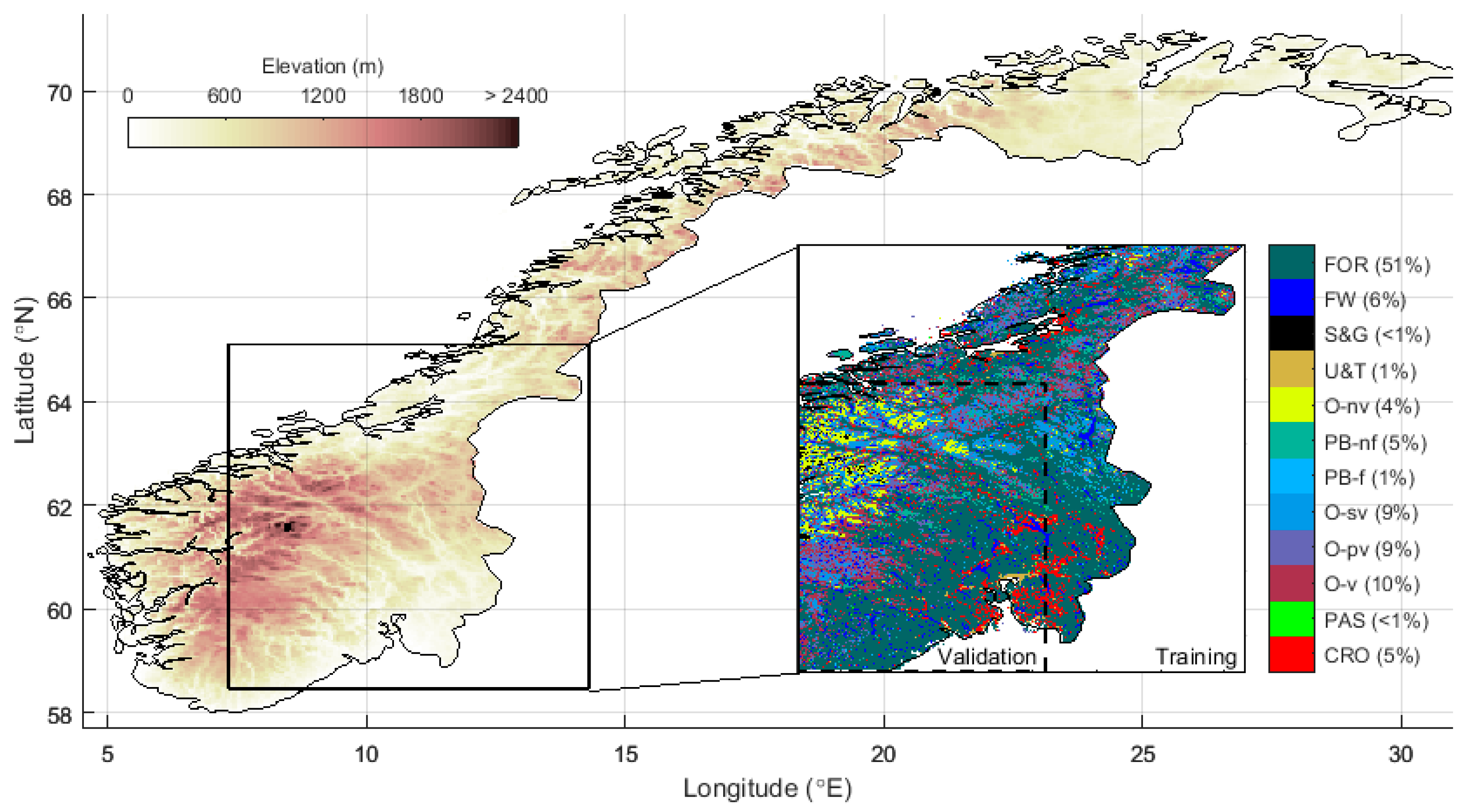
The general workflow is divided into two parts: (i) model training and (ii) model validation. Both are limited to the southern portion of mainland Norway (Figure 1) in order to include a larger wintertime sample of good quality MODIS snow cover and surface albedo retrievals (described in Section 2.5 and Section 2.6) since these have a low frequency at higher latitudes during winter. Furthermore, the study region contains the full range of land cover and climate variation found in Norway (Figure S6 of Supporting Information).

2.1. Study Region

Forests make up the dominant land cover type within the study domain, which covers a region with a total land surface area of approximately 167,500 km2 (Figure 1, inset). As such, preserving a similar proportion of forest area between the model training and validation regions was the main criterion when partitioning the domain into the training and validation subsets. Most of the forests within the full domain may be considered part of the boreal forest belt that extends almost continuously around the upper northern hemisphere. Forests are dominated by Norway spruce (Picea abies H. Karst.), Scots pine (Pinus sylvestris L.) and two birch species (Betula pendula Roth and B. pubescens Ehrh.), with the understory vegetation typically dominated by ericoid dwarf shrubs (Vaccinium spp.) and various herb communities [30].
The eastern parts of the region experience continental climates that are characterized by long cold winters, short mild summers and moderate, seasonally distributed precipitation. Forests in the northwestern coastal regions are more influenced by an oceanic climate, which is characterized by greater amounts of precipitation, warmer temperatures during winter, and cooler temperatures during summer. Snow covers the ground from December through late March/early April in the lowland regions (< 400 m). At higher elevations (> 600 m), permanent snow cover may commence in November and can persist through early May (Norwegian Meteorological Institute, 2013b).

2.2. Spectral Unmixing Regression Analysis

Satellite retrievals of the surface albedo are often provided at a spatial resolution that is too coarse for direct attribution to individual forest stands and other fine-scale features of the landscape. For instance, the nominal spatial footprint of the MODIS albedo product employed in this study (described in Section 2.5) is 25 hectares (250,000 m2), whereas the footprint of the typical even-aged forest stand in Norway rarely exceeds 1–2 hectares (< 20,000 m2) [31]. Linear spectral unmixing techniques based on the ordinary least squares regression are increasingly employed to overcome this spatial mismatch challenge (e.g., refs. [32,33,34]). Unlike conventional spectral unmixing techniques based on linear mixture models [35] in which the endmember spectral signatures are known a priori and the goal is to determine endmember fractions within any given pixel, the known endmember fractions in the present study are obtained from the land cover dataset, which are used to estimate their unique spectral signatures (albedos).
Under the premise that the surface albedo (or rather the surface reflectance) signal registered by the satellite spectroradiometer represents a linear combination of the individual albedos (reflectances) of all endmembers (land covers/forest stands) within its footprint, the linear unmixing model may be described [32] as:
α + ε α = i = 1 n ( e f i ( α i + ε i ) )
where α is the albedo of the grid cell (described in Section 2.5), e f i is the fractional coverage of endmember type i within the pixel size (Section 2.3), α i is the albedo of endmember i, ε α is the residual error of the pixel, and ε i is the standard error of the estimator ( α i ). In Equation (1), the endmember albedo α i is essentially the slope that minimizes the sum of squared ε α .
Endmember albedos α i are highly sensitive to the presence of snow. Equation (1) is therefore modified following Bright et al. [34] where α is described as a weighted combination of the mixed endmember albedos under snow-free and snow-covered conditions, with the weights determined by snow cover:
α = S C i = 1 n e f i ( α s c , i ) + [ 1 S C ] i = 1 n e f i ( α s f , i )
where α is the albedo of the grid cell (described in Section 2.5), SC is the snow cover of the grid cell (described in Section 2.6), and α s c , i and α s f , i are the albedos for endmember i under snow-covered and snow-free conditions, respectively. This model form is used in some climate models [36] and has been found to perform consistently well over large spatial domains at high latitudes [34,37]. Unlike in Bright et al. [34], however, the model employed here is further modified to capture additional variation in endmember-dependent albedos— α s c , i and α s f , i —owed to important local differences in vegetation structure and other environmental factors as described below.
For the vegetated endmembers and in particular forests, both α s c , i and α s f , i are influenced by the structure of the vegetation. In Fennoscandic boreal forests, α s c , i and α s f , i at the stand level have been found to be negatively correlated with canopy cover [38], leaf area index [38,39], aboveground biomass [38,40], volume [41], height [41] and age [27,33]. Because forest canopies are rarely fully buried by snow, ground masking by forest canopies is particularly influential as a control of surface albedo during the snow season [16,18,42], although the snow intercepted and held by forest canopies can be important during the coldest and calmest winter months [43,44,45].
Following Kuusinen et al. [33], we modeled the forest endmember albedos as functions of stand structure. Although the models of Kuusinen et al. [33] were fit separately for different seasons, it was possible to obtain universal endmember models that were not specific to individual months or seasons by including snow cover as an environmental state predictor. The albedo of an endmember under snow-covered conditions ( α s c , i ) is largely determined by the albedo of snow, which depends on the effective snow grain area and snow water content [46,47,48,49]. These are two physical properties that exhibit strong relationships with air temperature [50,51]. Furthermore, given the importance of air temperature as a control over vegetation phenology [19,52,53] and canopy snow dynamics (i.e., snow slippage and melt) [39,44,45,54], we included air temperature as an additional environmental state predictor.
For the forest endmembers, a model function was chosen that gives identical predictions for a zero structure forest—or when the structural predictor (i.e., volume, biomass, age and so on) equals zero. In other words, the forest endmember models have common y-intercepts. For snow-covered conditions, the functional form of the forest endmember model is given as:
α s c , i ( x i , T ) = ( α 0 , s c + ρ 0 , s c T ) ( β s c , i + ρ s c , i T ) [ 1 e λ s c , i x i ]
where T is the air temperature (in °C) of the grid cell (Section 2.7), α 0 , s c is the y-intercept (albedo) for forests with zero structure and when air temperature equals zero, ρ 0 , s c is a temperature sensitivity parameter for forests with zero structure, β i is the difference between α 0 , s c and the minimum albedo (i.e., the asymptote) for forest endmember i when air temperature equals zero, ρ s c , i is a temperature sensitivity parameter unique to the forest endmember i; λ s c , i is a shape parameter unique to the forest endmember i; and xi is the grid cell mean stand structural attribute for the forest endmember i (Section 2.4). Here, separate fits are performed using either the mean stand volume (x = Volume; m3 ha−1) or mean stand aboveground biomass (x = Biomass; t ha−1) as structural predictors.
The same function represented as Equation (3) was applied to estimate the forest endmember albedos under snow-free conditions:
α s f , i ( x i , T ) = ( α 0 , s f + ρ 0 , s f T ) ( β s f , i + ρ s f , i T ) [ 1 e λ s f , i x i ]
where the subscript “sf” denotes snow-free conditions.
In Equations (3) and (4), the zero-structure y-intercept parameter α 0 shared by all forest endmembers was based on the mean of the forest endmember-specific zero-structure y-intercept parameters obtained from an initial regression analysis (i.e., α 0 = i = 1 n α 0 , i / n ).
Air temperature modifiers were also included for the non-forested endmembers given its importance as a control over seasonal phenology (i.e., vegetation dynamics) and snow physical processes (i.e., snow albedo):
α s c , i ( T ) = α 0 , s c , i + ρ s c , i T α s f , i ( T ) = α 0 , s f , i + ρ s f , i T
where the intercepts α 0 , s c , i and α 0 , s f , i are the surface albedos for endmember i under snow-covered and snow-free conditions when air temperature equals zero, respectively, while ρ s c , i and ρ s f , i are air temperature modifiers for endmember i (i.e., slopes of the albedo–air temperature relationship).
Separate models were fit for both intrinsic albedos (black-sky/directional hemispherical and white-sky/bidirectional hemispherical) at the local solar noon and for each broad spectral band: visible (VIS; 300–700 nm), near infrared (NIR; 700–5000 nm) and the entire shortwave broadband (SW; 300–5000 nm).

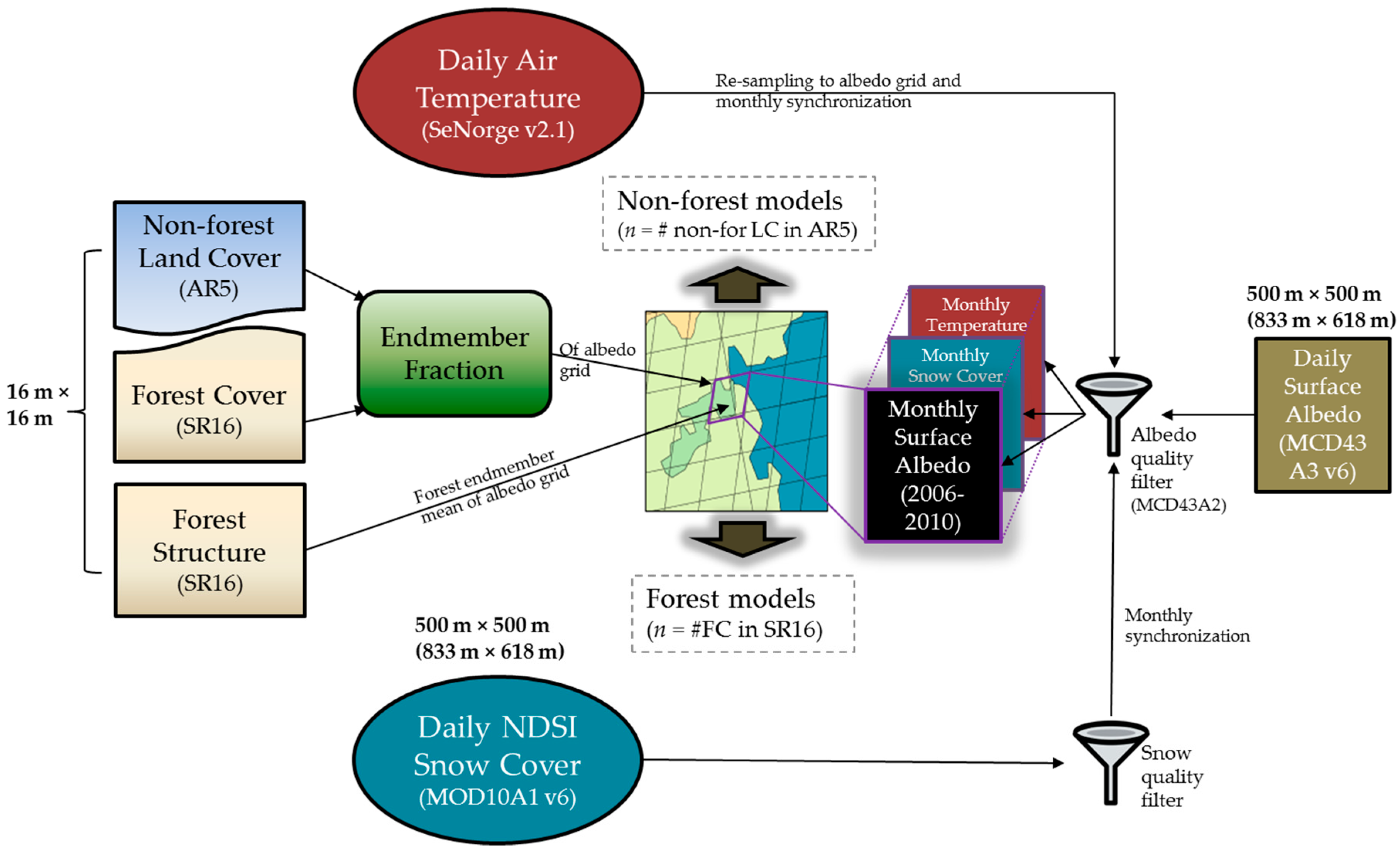
2.3. Land Cover Data

Endmember (land cover) mapping employed in model fitting was based on the high resolution land resource database “AR5”, which employs a standardized Norwegian land cover classification system [55]. Although AR5 is a national seamless database, detailed information about land resources is only available for areas below the treeline. As a result, a recent mapping campaign for areas above the treeline was recently undertaken, resulting in a complimentary database “AR-Fjell” [56]. Furthermore, an additional campaign to improve the mapping of agricultural resources was more recently carried out, resulting in the database “FJB-AR5” [57]. These products, which were all produced at a scale of 1:5000, were merged and re-projected to a MODIS sinusoidal grid with a resolution of 16 m × 16 m.

2.4. Forest Cover and Structure Data

The forest species composition and structure employed in model fitting were based on the forest resource map “SR16”, which was developed using photogrammetric and LiDAR point cloud data with ground plots from the Norwegian National Forest Inventory (NFI) [58]. The forest cover in SR16 is based on updating the forest cover in AR5 with object-based image analysis methods [59]. Stand attributes, such as tree species, tree height (Lorey’s), biomass, and volume are predicted with generalized linear models at a resolution of 16 m × 16 m with an accuracy (normalized RMSE) of 50% [58]. The forests in SR16 are classified as one of four classes: (1) newly clear-cut; (2) spruce; (3) pine; and (4) deciduous broadleaf. Pixels that were classified as newly clear-cut comprised ~1% of all forested pixels in the training dataset and were thus re-classified as spruce since spruce was the most abundant tree species of the model training region.
After fitting the models (Section 2.2), they were applied to reconstruct the monthly mean surface albedos in the validation region (Figure 1). Because the SR16 product used in the fitting did not yet extend to this region of Norway, an alternative product “SAT-SKOG” [60] was instead used in order to provide information about the forest cover and structure. The SAT-SKOG product is based on a k-nearest neighbor algorithm, which combines the spectral information from Landsat 5 & 7 with information from permanent NFI plots [60,61]. The structural variables in the SAT-SKOG product are limited to stand volume and height; thus, only the forest models fit using the stand volume as the structural predictor (i.e., x i ) were applied in the validation exercise. The forest area in AR5 and SAT-SKOG are identical so only the species information in SAT-SKOG was used to update the AR5 classification for forests. The SAT-SKOG forest classification differs from SR16 in that it includes a “mixed evergreen needleleaf” and a “mixed needleleaf-broadleaf” classification. For the former, we weighted the pine and spruce endmember predictions evenly while for the latter, we weighted predictions for all three species (spruce, pine, birch) evenly.

2.5. Albedo Data

The albedo data employed in fitting and validation were based on the MODIS Bidirectional Reflectance Distribution Function (BRDF) and Albedo Product (MCD43) algorithm utilizing directional surface reflectance values [62,63] from both the Aqua and Terra satellites [64,65] and a semi-empirical kernel-driven BRDF model (Ross-thick, Li-sparse Reciprocal) [66]. Specifically, we employed the latest version (v6) of the MCD43A3 BRDF/Albedo product with a nominal spatial resolution of 500 m in a sinusoidal projection (tiles v2 h18 & v3 h18), which is now provided at a daily resolution [67]. Although they are now provided at a daily resolution, the v6 MCD43A3 product retains the 16-day observation window where the observations closest to the composite date (9th day) are given a greater weight in determining the appropriate reflectance anisotropy model (i.e., BRDF) [68]. The accuracy of the v6 product is generally higher for snow-free and full inversion retrievals, with RMSEs < 0.02 for most land cover types. For snow-covered conditions, RMSEs are typically < 0.05 for most land cover types [69]. Furthermore, the v6 product obtains more retrievals than the v5 product at higher latitudes from the use of all available observations (as opposed to four observations per day in v5) [69].
The albedo data were downloaded for a temporal extent spanning 1 January 2006–31 December 2010. This temporal extent was chosen because it falls in between the earliest satellite imagery underlying the original AR5 product (2002) and the latest aerial remote sensing data used to produce the SR16 product (2014). The quality flags of the MCD43A2 [70] companion product were used to filter and discard all non-full BRDF inversions, which includes those with solar zenith angles greater than 70°. Data were then averaged into interannual monthly means, and composite dates and locations for the good quality data were stored for subsequent temporal synchronization with the snow cover and temperature data (next sections).

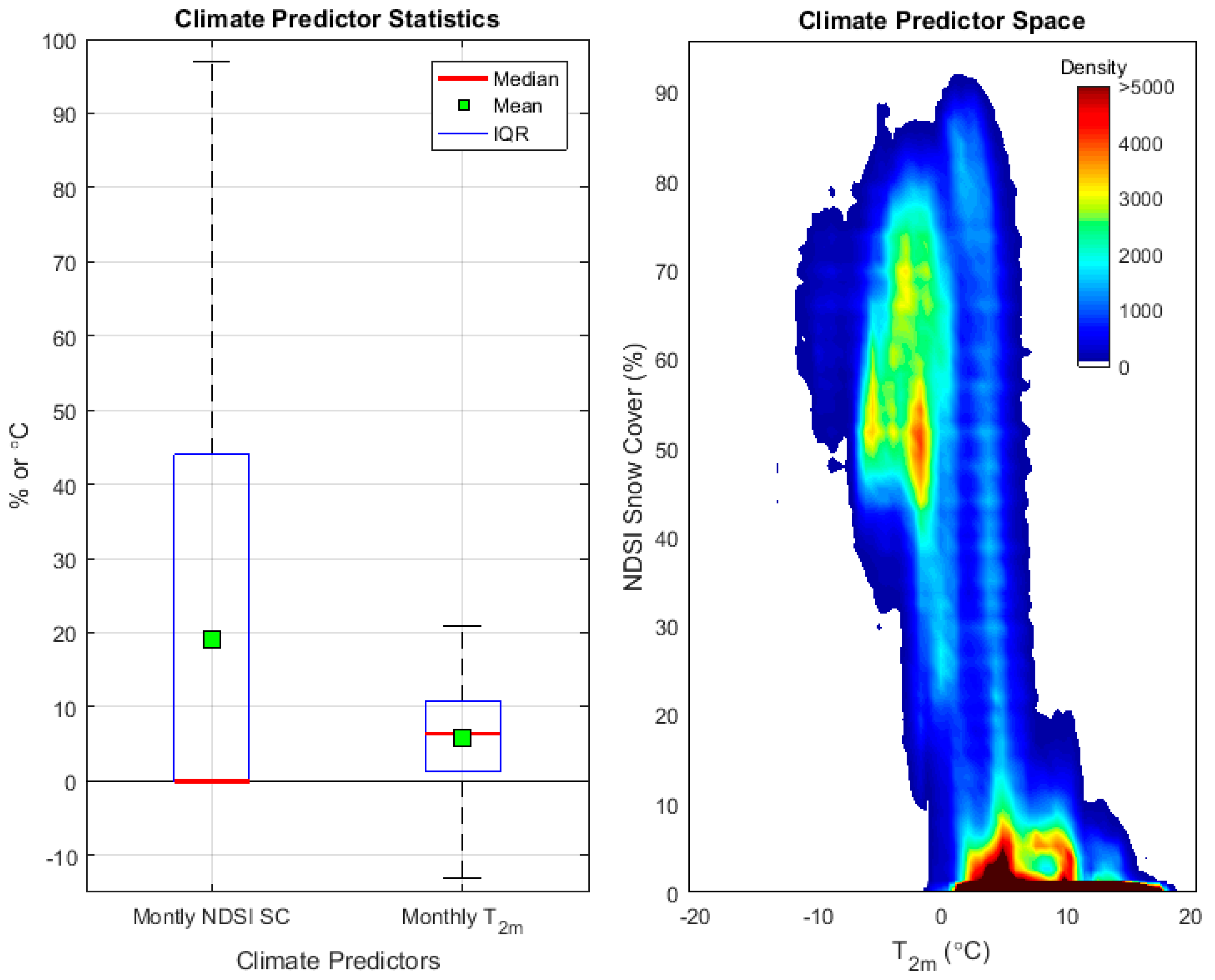
2.6. Snow Cover Data

The snow cover data for the same temporal extent as the albedo data were based on the latest version (v6) of the MOD10A1 Snow Cover product [71], which is also provided at a daily resolution and has a nominal spatial resolution of 500 m in a sinusoidal projection. Unlike the previous product (v5), only the Normalized Difference Snow Index (NDSI) Snow Cover [72] is provided. The NDSI Snow Cover represents the visible fraction of a grid cell covered in snow and rarely exceeds 0.75 in forests. The detailed descriptions of the v6 product, including other important changes from v5, may be found in refs. [73,74]. Recent evaluations suggest notable improvements in the v6 product over v5, which is largely due to refinements in the snow detection algorithm [75,76]. Evaluations at three locations after the conversion of NDSI Snow Cover to Fractional Snow Cover using linear regressions with global parameters suggest an accuracy (RMSE) of 0.2–0.35 [75]. Prior to aggregating these to multi-year monthly means, the temporal signature of the snow cover data was synchronized to match that of the albedo dataset. In other words, the quality flags of the albedo dataset were applied to filter and discard snow cover retrievals for dates that did not correspond to the dates of the retained good quality albedo retrievals. NDSI snow cover (henceforth referred to as simply snow cover; SC) values outside the 0–100 range were also discarded prior to the application of the albedo quality filter.

2.7. Temperature Data

The monthly mean temperatures from 2006–2010 were based on 1 × 1 km grids of daily (24-hr) mean air temperatures (2 m) created from three-dimensional spatial interpolation of air temperatures observed at meteorological stations distributed throughout Norway [77]. The accuracy of the gridded daily temperature product (SeNorge 2.0) is ~1 °C based on the “leave-one-out” cross validation score [77]. Temperature data were re-projected and downscaled to the nominal resolution of the MODIS products using a nearest neighbor interpolation method. The same temporal synchronization procedure that was applied to the snow cover data was applied to the temperature data prior to monthly aggregation.
Figure 2 provides an overview of the climate predictor space of the model fitting domain associated with the post-processed dependent variable (albedo) dataset.
Monthly mean air temperatures rarely fell below −10 °C, with a median close to the mean of ~6 °C (Figure 2, left panel). Over 75% of the monthly mean snow cover (SC) retrievals had values less than 44%, with a median of 0% and mean of ~19%. It is important to note that the highest SC values were not necessarily found in the coldest months but in months where the mean T was around 2–4 °C. These temperatures are characteristic of late winter/early spring when the snowpack is near its deepest (i.e., when a larger amount of short-statured vegetation or other landscape features are buried in snow) [78].

2.8. Endmember Data Processing

Prior to calculating the endmember fractions ( e f i ) corresponding to each MODIS product grid cell, the original forest area of the AR5 land cover product was replaced by the updated area of the SR16 product. It is becoming increasingly understood that the effective spatial resolution of the MCD43A BRDF/Albedo product differs from its nominal resolution of ~500 m [15,68,79]. Recently, Campagnolo et al. [80] applied point spread functions to quantify the effective spatial resolution of various MODIS and other optical satellite remote sensing products. For the v6 MCD43A BRDF/Albedo product, they reported a median effective resolution of 833 m along the east–west transect and 618 m along the north–south transect.
Endmember fractions were computed at both the nominal (500 m × 500 m) and the effective (618 m × 833 m) resolutions before model fitting was executed for both resolutions. Similar to Hovi et al. [81], we apply an elliptical point spread function modeled with a Gaussian distribution, which was defined such that 75% of the signal was assumed to originate from within an ellipse having a diameter of 618 m in the Y (north–south) and 833 m in the X (east–west). Forest structural predictors (Section 2.4) were computed as the weighted means within each pixel using the point spread function as weights, which is illustrated conceptually in Figure S5 of the Supporting Information.
The general workflow of the entire linear unmixing (model fitting) procedure is illustrated in Figure 3. Figure S1 of the Supporting Information provides an overview of the distribution of the quality-filtered and temporally-synchronized observational records employed in model fitting and validation by land cover (endmember) type and month.

2.9. Model Validation
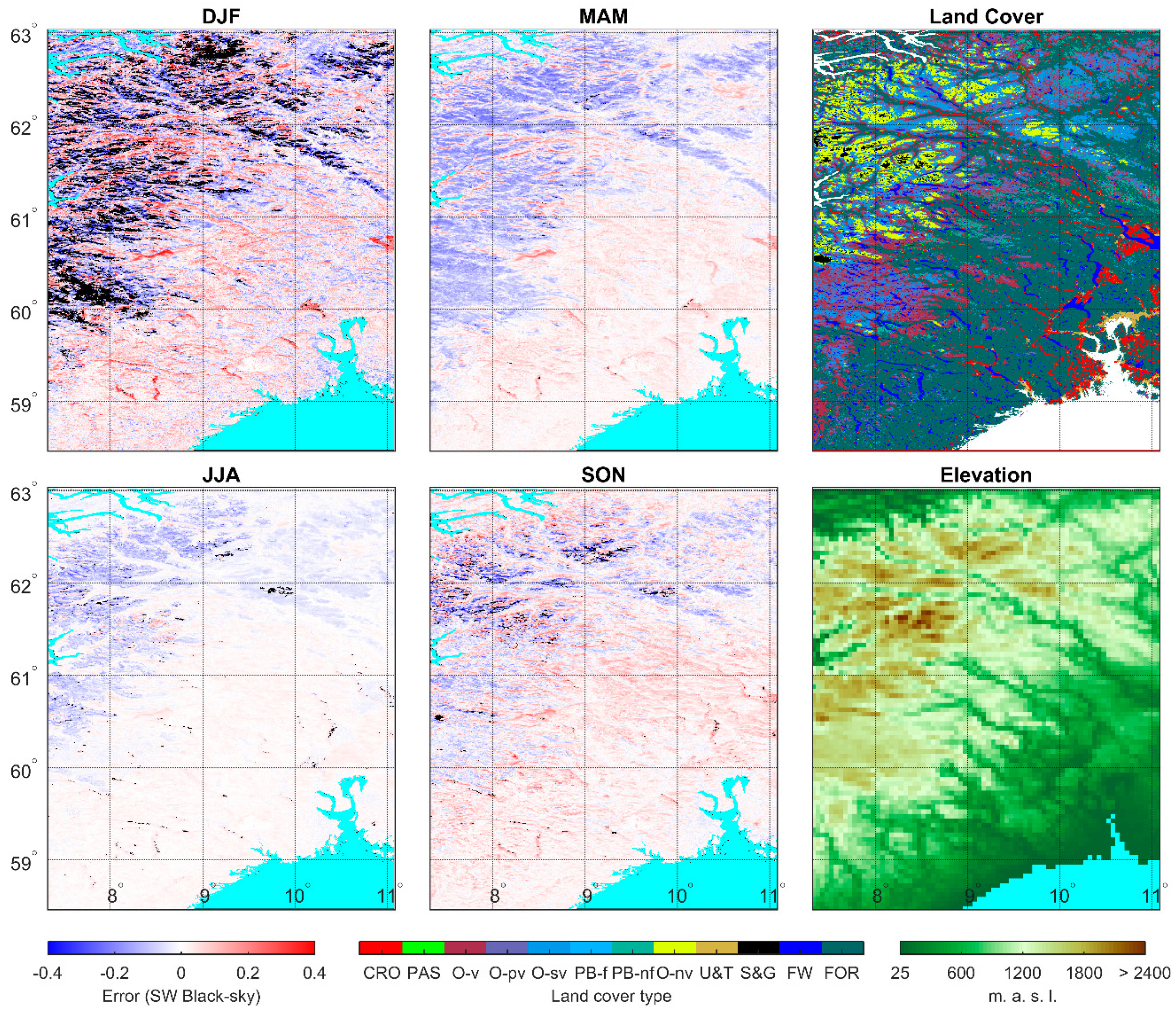
Pixel errors (E) for all broad bands and for both intrinsic albedos were calculated as the difference between the predicted and MCD43A albedo retrievals (both at the local solar noon):
E p , m = α ¯ p , m α p , m
where α ¯ p , m is the predicted and α p , m is the MCD43A albedo retrieval for month m and pixel p. Because our main interest was to assess the prediction performance of the individual endmember (land cover type) models, we limited the validation sample to a subset of pixels containing homogeneous land cover—defined here as those whose total area contained ≥95% of a single endmember type.

3. Results

3.1. Fit Statistics

The relevance of including both air temperature and forest structure as predictor variables can be appreciated when looking at the coefficients of determination (R2), which are presented in Table 1. Although snow cover (SC) alone explained 55–81% of the variance (depending on model complexity and albedo broad band), the addition of both air temperature and forest structure (volume or biomass) further increased the percentage of variance explained to 85–88%.
In general, for any given model permutation, the fits for the VIS broad band explained more of the variance than the fits for SW and NIR broad bands. Furthermore, the fits for black-sky albedo explained more of the variance than the fits for the white-sky albedo (Table 1). The models fit at the effective spatial resolution did not lead to as large R2 improvements as those reported elsewhere [81], although it should be noted that the study of ref. [81] was restricted to forests where there is a much larger variation in vegetation structural controls of the surface albedo.

3.2. Model Parameters

Only the results for the black-sky albedos are presented henceforth. For other results, please refer to the Supporting Information. Starting with non-forest land cover types, the regression parameters for the three broadband albedos (black-sky) at the local solar noon are presented in Table 2. The zero degree albedos (all bands) under snow-covered conditions ( α 0 , s c , i ) were generally highest for the “Open” and “Peat bog” land cover types.
For shortwave (SW), zero degree albedos under snow-free conditions ( α 0 , s f , i ) were lowest for the two non-vegetated categories (“U&T” & “FW”). Snow-free albedos for the near-infrared (NIR) broad band tended to increase with increasing vegetation cover. For instance, NIR α 0 , s f , i was higher for forested peat bogs (“PB-v”) than for non-forested peat bogs (“PB-nf”), and higher for vegetated open (“O-v”) than for partly or sparsely-vegetated open land cover types (“O-pv”, “O-sv”). The influence of vegetation on α 0 , s f , i was less clear for the visible (VIS) broad band. For non-vegetated open areas (“O-nv”) which typically reside at the highest altitudes, α 0 , s f , i was higher than that of fully vegetated open areas (“O-v”) and of vegetated peat bogs (“PB-f”).
For all land cover types (endmembers) and for all broad band albedos, the parameter relating the endmember albedo under snow-covered conditions to the monthly air temperature (i.e., ρ s c , i ) was negative, which is consistent with numerous observations elsewhere [47,50,51,82,83]. For the croplands and pastures occupying lowland regions, ρ s f , i for the SW albedo was positive and appeared to be driven by the positive ρ s f , i for the NIR albedo. For “Open” and “Peat bog” cover types, ρ s f , i for SW was negative and appeared to be driven by a negative ρ s f , i in the VIS band.
For forested endmembers, the parameters for the models that were fit with the stand volume as the structural predictor (xi in Equations (3) and (4)) are presented in Table 3. Under snow-covered conditions, α 0 was highest for VIS and lowest for NIR broad bands while the opposite was true for snow-free conditions. The magnitudes of the zero structure forest temperature sensitivity parameter ρ 0 follow the same pattern. Under snow-covered conditions, the difference in the albedo between a zero structure and a fully developed forest when air temperature is zero (i.e., β s c ) was largest in the VIS band and smallest in the NIR band, whereas the opposite was true for snow-free conditions ( β s f ). Under snow-covered conditions, the difference in the albedo between a zero structure and a fully developed forest decreased with decreasing air temperature, which provided positive values for ρ s c for all forest endmembers and albedo bands. The lack of foliage during the months with snow at the surface likely explains why the temperature sensitivity parameter ρ s c was larger (in magnitude) for the deciduous endmember (“DBF”) than for pine and spruce.
As for the snow-free temperature sensitivity parameter ρ s f , the values in all bands were negative for the spruce and pine endmembers. However, we found positive ρ s f values for DBF in the VIS band. A likely explanation is that the leaf area tends to increase with increasing temperature, and for DBF, the VIS albedo of Betula spp. bark and branches (especially in the green (560 nm) and red (660 nm) bands [84]) is higher than that for foliage [85,86]. The positive ρ s f in the VIS band appeared to outweigh the negative ρ s f in the NIR band, resulting in a positive ρ s f for the entire SW broadband albedo (Table 3).
The shape parameters λ s c and λ s f in each broad band were similar in sign and magnitude for all the endmembers and were largest in the VIS band. The negative values suggest that the albedos decreased with increasing aboveground volume (or biomass), and that the total surface albedo was driven by the canopy masking of the ground surface and understory. This result can be more fully appreciated when looking at Figure 4.

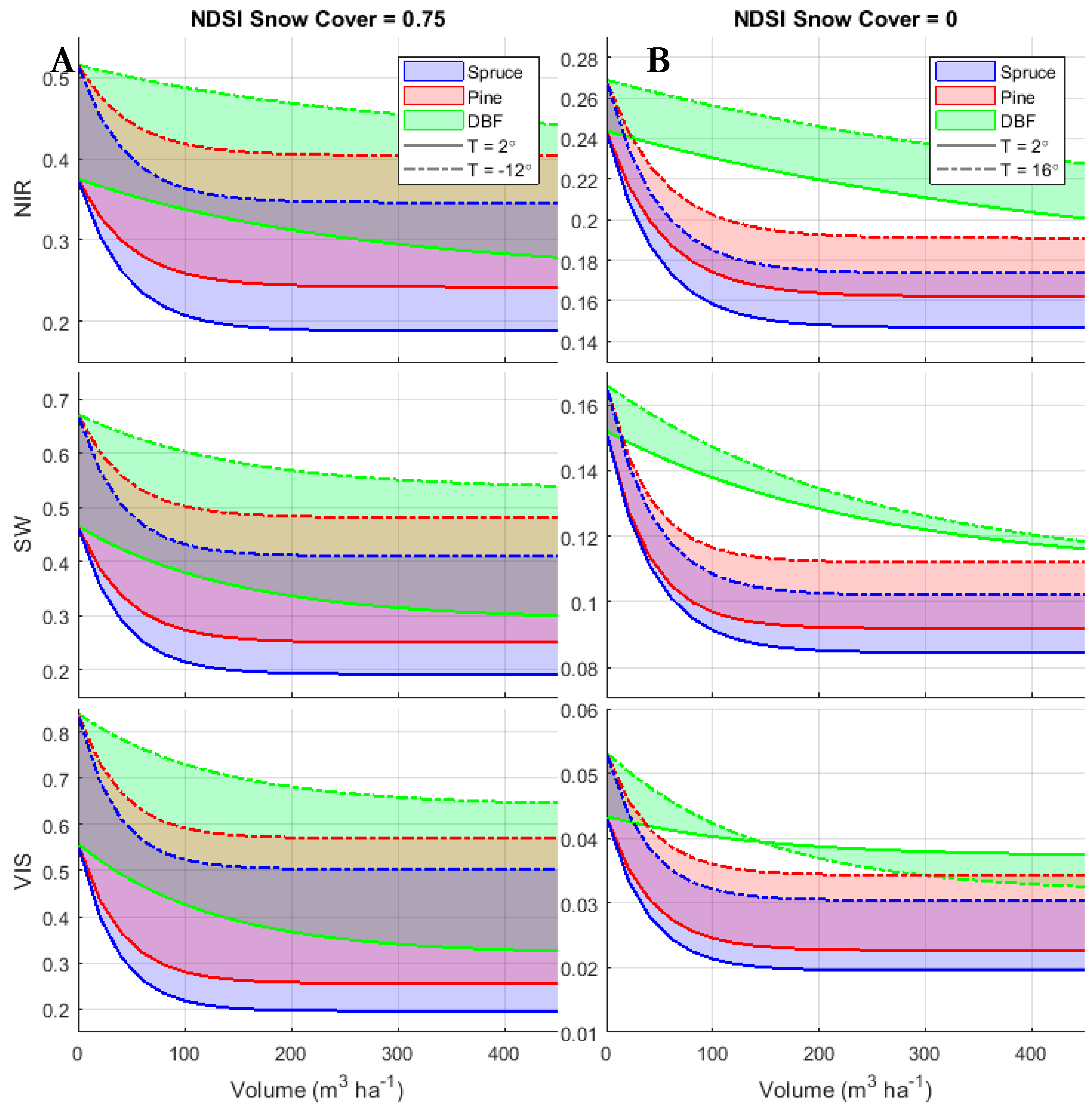
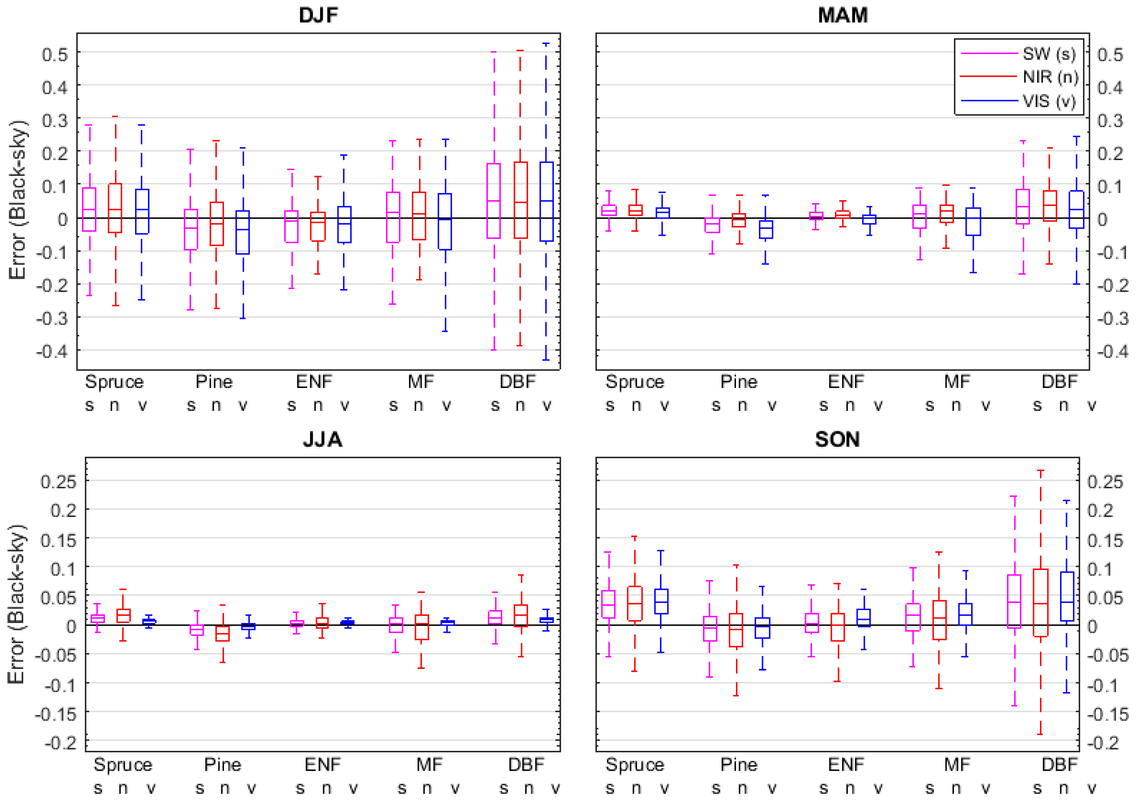
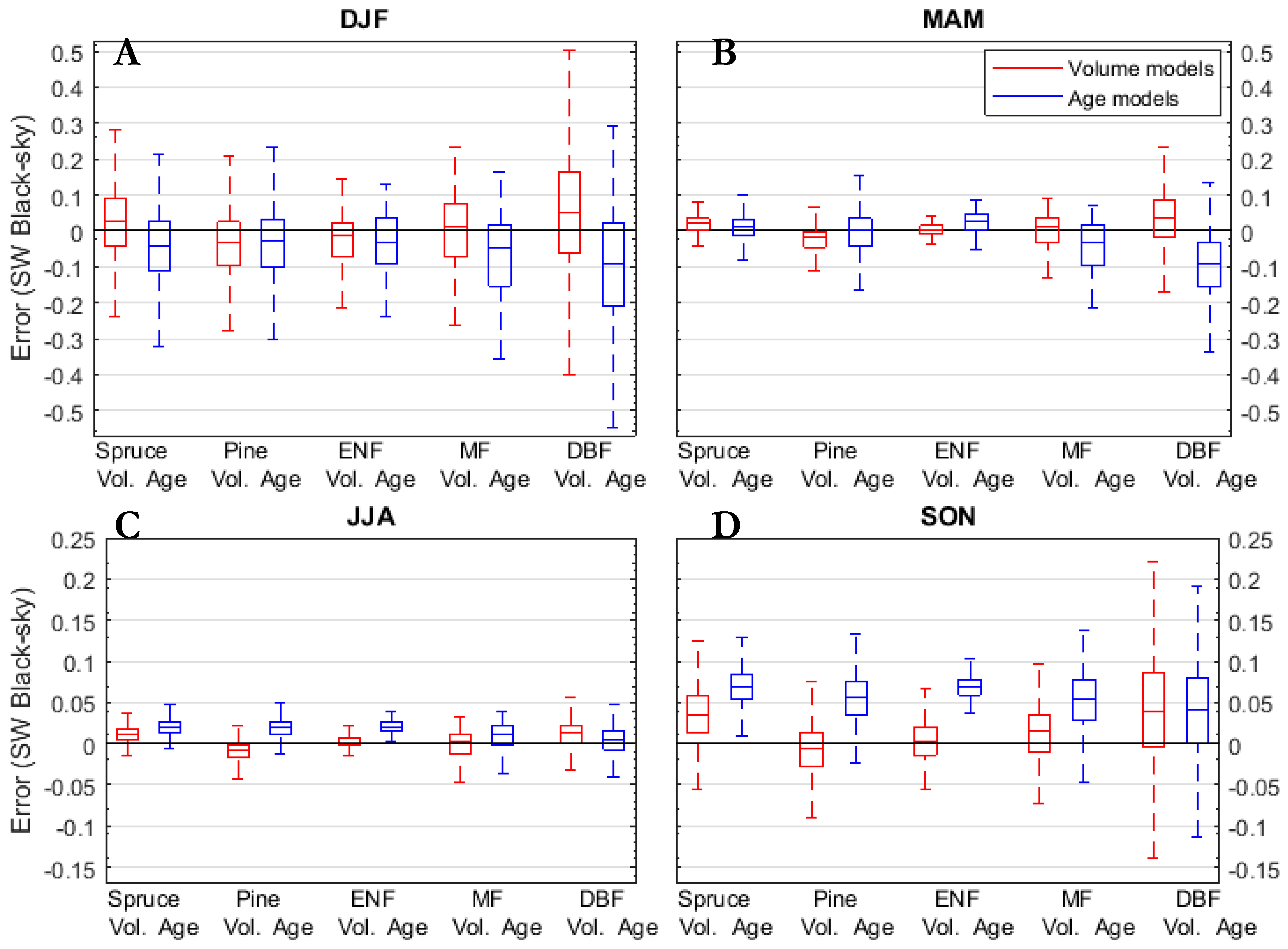
3.3. Model Behavior in Forests

For forests, the model behavior under both snow-covered and snow-free conditions is only presented for the volume models (Figure 4) although the models behaved similarly for biomass (Supporting Information Figures S3 and S4). To illustrate this behavior, we fixed SC at two extremes —0.75 (snow-covered) and 0 (snow-free)—and two temperature extremes at these two SC extremes. The shaded area between the solid and dashed curves in Figure 4 illustrates the effect of the temperature sensitivity parameter.
The albedo in all broad bands increased with decreasing temperatures during the snow season. The factors that were likely contributing to the differences between the −12° and 2° curves shown in Figure 4A were the amounts of snow intercepted and held by forest canopies and the physical properties of snow itself. For instance, when the monthly SC is 0.75 and monthly T is −12 °C, the monthly albedos of a young or newly harvested stand (i.e., when volume = 0) can be as high as 0.86, 0.67 and 0.54 for the VIS, SW and NIR bands, respectively. These values reduce as the forests age and the stand volume (or aboveground biomass) increases. For the pine and spruce endmembers, Figure 4A suggests that the albedo varies only slightly above ~150 m3 ha−1. However, the asymptotic albedo is not reached within the plotted range for DBF (i.e., 450 m3 ha−1).
Turning our attention to the forest endmember model behavior under snow-free conditions (Figure 4B), the albedos were highest in the NIR band and lowest in the VIS band. In all broad bands, the albedos were generally highest in DBF and lowest in spruce. The albedo variation with temperature is represented by the shaded areas and is largest for the NIR band. For the spruce and pine endmembers, the highest albedos for any broad band corresponded to the warmest periods. However, the VIS albedo (Figure 4B, solid curve) was highest when the air temperatures were lowest for DBF (i.e., during the shoulder seasons). This may be explained by the lack of foliage that exposed light-colored stems, which are characteristic of the birch species (Betula spp.) in our study region. This was in contrast to the relationship between the temperature and NIR albedo where, similar to pine and spruce, the NIR albedos for DBF were highest during the warmest periods (Figure 4B, top panel, dashed green curve). This contrast results in a much narrower range of SW albedo for DBF under snow-free conditions (Figure 4B, middle panel, green shaded area), particularly at high stand volumes. The range of the albedo variation with temperature is larger for all tree species for the white-sky albedos (Supporting Information Figures S2 and S4).

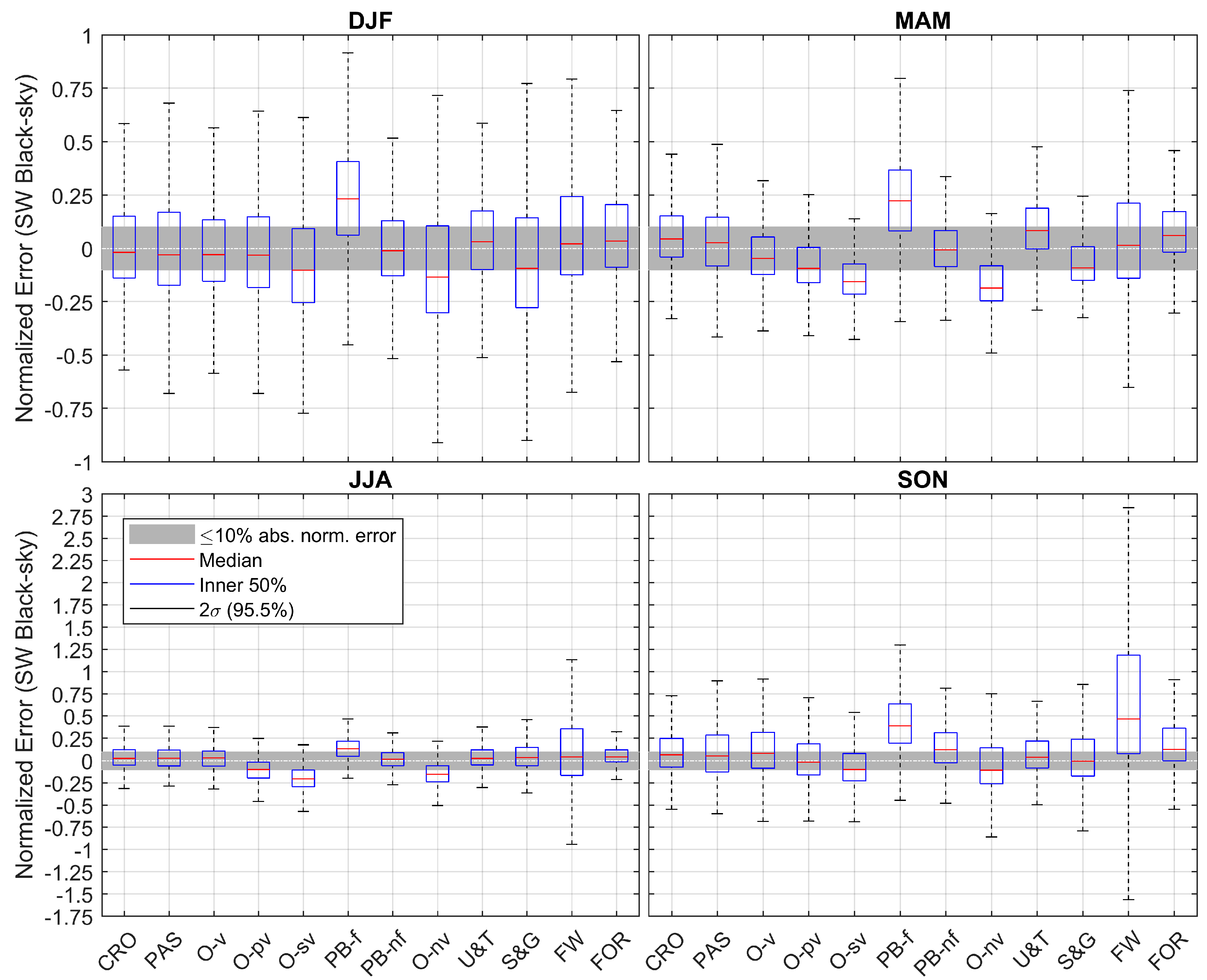
3.4. Model Benchmarking and Validation

Given their slightly higher accuracy, only the prediction error for the models fit at the effective spatial resolution is presented henceforth. Starting at the pixel level, Figure 5 illustrates the geospatial distribution of the seasonal error (SW broadband, black-sky) within the validation region. The largest errors in all seasons were mostly confined to the higher elevation regions of the north and west. The largest errors were found in winter (DJF) in these regions—regions with monthly T and SC values at the edge of or exceeding the range found in the model training region. In general, the largest positive errors (red values, Figure 5) in winter were found over the largest inland waterbodies (“FW”). Although this error was reduced, the positive error seen over larger freshwater bodies was also evident in spring (MAM) and autumn (SON). On average, the mean SC over these larger freshwater bodies during the colder seasons in 2006–2010 was found to be lower than for the smaller freshwater bodies, which resulted in overestimates of the surface albedo when combined with a low temperature sensitivity parameter ( ρ s c , Table 2). For all seasons, the larger negative errors (blue values) were typically found for pixels with larger proportions of the two open area types “O-nv” and “O-sv”, which were mostly concentrated at the higher elevation regions of the north and west (Figure 5, third column of sub-panels).
Moving on to forests, the seasonal prediction errors in the validation domain for the volume-based models are reported in Figure 6 for all bands. The largest errors were found in winter (“DJF”; Figure 6) for DBF where the variations in structure not explained by stand total volume were larger than in snow-free seasons. In winter, the DBF model had a high prediction error, with a median of ~0.05 for all bands. The absolute error for 50% of the predictions (i.e., the interquartile range) for all bands fell within ~0.07–0.17. For other forest types, the median and interquartile errors were smaller. A median positive error of ~0.025 (all bands) was found for spruce. For pine, the median errors were negative for all bands although this error was lower for the NIR band. Combining the parameters for pine and spruce resulted in the lowest median and interquartile error ranges for mixed-conifer forests (“ENF”). Although the median errors were equally low for mixed forests (“MF”), the error interquartile ranges were approximately double that of ENF. For SW, the mean of the median errors for all forest types was 0.01, or ~3% of the mean SW albedo of forests during DJF.
Turning our attention to spring (Figure 6; “MAM”), median prediction errors in all forests were found to be similar to those in DJF. However, a major difference was that errors in MAM were much more tightly distributed around the median values. In other words, the error interquartile ranges in MAM were approximately 25–40% of those found for DJF. The improved accuracy in MAM was unsurprising given that a larger share of the high quality MCD43A retrievals representing snow-covered conditions stemmed from MAM, thus influencing the snow-covered model parameters more heavily. Similar to DJF, the largest errors in MAM were found in DBF and MF. For SW, the mean of the median errors for all forest types was 0.01, or 4.5% of the mean SW albedo of forests during MAM.
The lowest errors were found during summer (“JJA”; Figure 6). Whereas median error and error interquartile ranges for the three broad bands were similar in magnitude for winter and spring, the median and interquartile errors in the NIR band in JJA were notably larger than that for the VIS band. For the SW band, the mean of the median error for all forest types was 0.0025, or ~2% of the mean SW albedo of forests during JJA.
As for JJA, the error interquartile ranges for the NIR band were larger than for the VIS band during autumn (“SON”; Figure 5). The spread in error in SON was second largest after DJF although median errors were similar. As for DJF and MAM, the spread in errors (interquartile ranges) was largest for DBF.
For all forested pixels included in the validation exercise, predictions (SW black-sky only) were also compared to predictions from the empirical models of Bright et al. [27] which were based on forest age and T (Figure 7).
Starting in winter (“DJF”; Figure 7A), compared to the Age-based models the Volume-based models presented in this work appeared to slightly improve the DJF accuracy in forests judging by the median errors, with the exception of pine. For pine, the median error using the Volume model was similar to that of the Age model. The spread in errors for the Volume models were similar to the Age models, although the error interquartile ranges appear to have been slightly reduced for pine, ENF and MF with the Volume models.
For spring (“MAM”; Figure 7B), the median errors for ENF, MF and DBF using the Volume models were notably reduced compared to the Age models. The error interquartile ranges were reduced for all forest types although for spruce and pine, the median errors were slightly higher (in absolute terms).
In summer (“JJA”; Figure 7C), the median prediction errors were noticeably reduced in most forest types compared to the Age models. The exception is DBF where the median error using the Age model was slightly lower than that of the Volume model.
The most notable improvements over the Age-based models were found in the autumn months (“SON”; Figure 7D), which demonstrates that while monthly mean T may be a good proxy for snow during winter and spring, it suffers as a proxy for snow during autumn. Relative to the Age models, the application of the Volume models led to large reductions in the median errors in all forest types with the exception of DBF, where the median errors were similar.
Shifting our attention to the non-forest endmembers and the limiting results presented henceforth of the full SW broad band, spreads in model errors were largest in DJF as expected (Figure 8, upper left panel). Median prediction errors were under 0.05 for all land cover types, except for “O-sv”, “PB-f” and “O-nv”. Median errors for “O-sv” and “O-nv” were negative for each season. Median error for “PB-f” was positive for all seasons although we note that the number of MCD43A3 retrievals containing “PB-f” homogeneity to ≥95% was limited to just three.
In order to more rigorously assess whether these error patterns were systematic, we relaxed the homogeneity requirement described in Section 2.9 and recomputed the error statistics for all pixels using the sub-MODIS pixel modes from AR5/SR16 to define the majority land cover type. Figure 9 contains the results after normalizing the seasonal mean prediction error to the MCD43A3 retrievals, which reinforces the above-mentioned results that error patterns for “PB-f”, “O-sv” and “O-nv” were indeed systematic.
Figure 9 also shows that the range in errors for freshwater (“FW”) relative to the retrieved values is the largest among all land cover types, particularly in autumn (Figure 9 SON and JJA, whiskers). Given an acceptable median error threshold of ≤10%, Figure 9 shows that all models except “PB-f”, “O-sv,” and “O-nv” are accurate in spring (MAM) and summer (JJA). In winter, median normalized errors of all models except “O-nv” and “PB-f” meet this accuracy threshold. For autumn, median normalized errors of all models except “PB-f”, “PB-nf,” and “FW” meet this threshold. Additionally, the large spread in error for “Birch” (Figure 6) causes the median normalized error for forests as a whole (“FOR” in Figure 9) to slightly exceed the 10% accuracy threshold.

4. Discussion

We combined a five-year climatology of the surface albedo, near-surface air temperature, NDSI snow cover and detailed maps of Norwegian land cover and structure to yield a set of empirical models giving estimates of the monthly mean surface albedo as a function of Norwegian land cover classification. Although the endmember fraction and NDSI snow cover alone could explain 55–81% of the variance in the land surface albedo in our model training domain (depending on which albedo and broad band one looks at), the addition of both air temperature and forest structure (volume or biomass) further increased the explained variance to 85–88% (Table 1). We consider this a remarkable outcome given the multiple sources of error inherent in the various land cover products employed in the model training exercise.
For non-forested vegetated land covers, we found strong relationships between air temperature and albedo (all bands), which suggests that tgrowing season phenology was sufficiently synchronized with monthly mean air temperatures. With the exception of croplands (“CRO”) and pastures (“PAS”), SW albedo (black-sky) decreased with increasing air temperature, suggesting that it was driven by increased vegetation masking of a higher albedo surface during the growing season. However, for cropland, pastures, and all forest endmembers, the SW albedo increased with increasing air temperature, suggesting either a larger role played by understory vegetation or by increased canopy masking of a lower albedo surface. During the snow season, we found that air temperature and surface albedo were negatively correlated. This is a relationship that is presumably driven by the influence of air temperature on snow metamorphosis and snow physical state [46,87]. When applied outside the training region, we found absolute normalized median errors to be ≤10% for most non-forest endmember models (SW black-sky). The non-forest endmember models on average performed best during spring (MAM) and summer (JJA) where the proportion of the total number of predictions agreeing within 10% of the MCD43A3 retrievals was around 35% and 45%, respectively (Figure S7, Supporting Information). These shares were weighed downward by the persistent positive error for forested peatbogs (“PB-f”) and persistent negative error for non-vegetated open areas (“O-nv”) whose proportions of the total number of predictions agreeing within 10% of the MCD43A3 retrievals were only 20% and 25% within the validation region, respectively (Figure S7). In general, these two land cover (endmember) types exhibit the largest variation in both geological attributes (exposed mineral composition) and vegetation attributes (vegetation cover fraction). These are two physical attributes important for the surface albedo which were not captured by the models. Furthermore, the model training region contained a disproportionately low share of “O-nv” relative to the validation region (Figure S1), and given the large variation in surface attributes within “O-nv”, a larger “O-nv” sample during model fitting would likely have resulted in an improved performance by this endmember model.
Our models were least capable of explaining variance in the NIR albedos, which is unsurprising given the large share of forest cover in the region and the large variation in foliage reflectance in the shortwave infrared (1.5–2.5 μm) band among Fennoscandic tree species [88]. This variation is likely attributed to differences in leaf-level functional traits [19,20,89], and although seasonal trends in air temperature likely explained some of the albedo variance linked to trends in the leaf area [26], such functional controls could not be accounted.
For the forest endmembers, the maximum and minimum albedo predictions under both snow-covered and snow-free conditions (Figure 4) appeared well-constrained when benchmarked to observations reported in other Fennoscandic regions based on satellite remote sensing [32,33,40,41,81]. The dependency of the albedo on forest structure was more difficult to compare quantitatively to the results of other studies since the environmental state conditions (i.e., SC and T) were often not reported alongside the reported results. However, qualitatively, the general relationship between forest albedo (all endmembers, all bands) and stand volume under snow-free conditions (Figure 4B) appeared be consistent with the regression fits based on the Landsat observations reported in Kuusinen et al. [41]. However, we did not find as strong a dependency as Kuusinen et al. [41] of the VIS broad band albedo on stand total volume (cf. Figure 1 in Kuusinen et al. [41]).
Under snow-covered conditions, the use of an exponential function to model the albedo-structure relationship in forests appeared appropriate when compared to that reported for Finnish forests for age (c.f., Figure 1 in ref. [33]) or biomass (cf. Figure 9A in ref. [40]). However, the shape parameters of our volume (Figure 4A) and biomass models (Figures S2 and S3) seemed to differ from the age-based models of Kuusinen et al. [33] where the asymptotic SW albedo value for DBF (birch) and spruce forests was reached around age 50 in ref. [31]. This is an age that corresponds to a stand volume and biomass in forests of our training domain for which the asymptotic albedo has yet to be realized. The behavior of the SW albedo model for DBF under snow-covered conditions reported in this study appears to be more consistent with the age-based DBF model of Bright et al. [27], which is unsurprising given the partly-overlapping model training domains.

5. Conclusions

We presented a coherent empirical modeling framework based on linear spectral unmixing of optical satellite retrievals of surface albedo. The unmixing framework allowed us to sample a relatively large area within a finite region of Norway containing multiple land cover features spanning large climate gradients. The unmixing approach may be computationally less expensive than the approaches based on homogenous pixel sampling, which often requires a more extensive spatial domain to be sampled in order to allow for a sufficient number of satellite retrievals. The resulting land (or vegetation) cover-dependent models developed and presented here can be applied to create a spatially-explicit surface albedo dataset (or database) for use in regional land-climate research and in climate-oriented land management planning in Norway. The models can also facilitate comparisons to land-cover dependent albedo predictions made by land surface (climate) models, which are difficult to evaluate by direct comparisons to satellite retrievals.
The models required just two environmental state predictors: monthly mean air temperature and monthly mean NDSI snow cover (SC), where the latter was also provided by optical satellite remote sensing. Given a normalized error threshold of ≤10%, most of the models proved to be accurate when validated against high quality MODIS albedo retrievals in a region outside of the model training region (based on the medians reported in Figure 9). The exception was the performance for forested peat bogs (“Pb-f”) and non-vegetated open areas (“O-nv”) whose normalized absolute median prediction errors exceeded 10% in all seasons. Although we reported a large range in upper and lower error quartiles for all models during winter months (DJF; Figure 6, Figure 7, Figure 8 and Figure 9), these larger errors may be deemed acceptable in most modeling contexts given the lower relevance of surface albedo during periods of low solar energy input (such is the case for Norway during DJF). Finally, although the MODIS NDSI-based SC can be higher than the 0.75 constraint shown in Figure 4, the higher values in our domain mostly coincided with the end of the snow season when the monthly mean T was also higher. We stress that great caution should be exercised when extrapolating the model behavior outside the extreme SC and T ranges presented in Figure 2.

Supplementary Materials

The following are available online at https://www.mdpi.com/2072-4292/11/7/871/s1: Table S1: Root mean squared errors of candidate models; Table S2: White-sky model parameters for forests with volume as structural predictor; Table S3: Black-sky model parameters for forests with biomass as structural predictor; Table S4: White-sky model parameters for forests with biomass as structural predictor; Table S5: White-sky model parameters for non-forest endmembers; Figure S1: Distribution of MODIS retrievals used in model fitting and validation by month and land cover type; Figure S2: White-sky model behavior for forests with volume as structural predictor; Figure S3: Black-sky model behavior for forests with biomass as structural predictor; Figure S4: White-sky model behavior for forests with biomass as structural predictor; Figure S5: Weighting scheme applied when fitting models to the effective spatial resolution; Figure S6: Distribution of Köppen-Geiger climate zones in Norway and within the study domain; Figure S7: Fraction of total predictions have ≤10% normalized absolute error (SW black-sky) by land cover type and season.

Author Contributions

R.M.B. conceptualized and designed the study, compiled and processed all data, carried out all modeling, analysis and validation, produced all figures and wrote the original manuscript draft. R.A. edited and commented on the original draft and R.M.B. and R.A. revised the final manuscript.

Funding

This research was funded by the Research Council of Norway (Norges Forskningsråd), grant number 255307/E10.

Conflicts of Interest

The authors declare no conflict of interest.

References

  1. Mahmood, R.; Quintanar, A.I.; Conner, G.; Leeper, R.; Dobler, S.; Pielke, R.A.; Bonan, G.; Chase, T.; McNider, R.; McAlpine, C.; et al. Impacts of Land Use/Land Cover Change on Climate and Future Research Priorities. Bull. Am. Meteorol. Soc. 2010, 91, 37–46. [Google Scholar] [CrossRef] [Green Version]
  2. Mahmood, R.; Pielke, R.A.; Loveland, T.R.; McAlpine, C.A. Climate Relevant Land Use and Land Cover Change Policies. Bull. Am. Meteorol. Soc. 2016, 97, 195–202. [Google Scholar] [CrossRef]
  3. Stephens, G.L.; O’Brien, D.; Webster, P.J.; Pilewski, P.; Kato, S.; Li, J. The albedo of Earth. Rev. Geophys. 2015, 53, 141–163. [Google Scholar] [CrossRef] [Green Version]
  4. Jackson, R.B.; Randerson, J.T.; Canadell, J.G.; Anderson, R.G.; Avissar, R.; Baldocchi, D.D.; Bonan, G.B.; Caldeira, K.; Diffenbaugh, N.S.; Field, C.B.; et al. Protecting climate with forests. Environ. Res. Lett. 2008, 3, 044006. [Google Scholar] [CrossRef] [Green Version]
  5. Pielke, R.A., Sr.; Marland, G.; Betts, R.A.; Chase, T.N.; Eastman, J.L.; Niles, J.O.; Niyogi, D.d.S.; Running, S.W. The influence of land-use change and landscape dynamics on the climate system: Relevance to climate-change policy beyond the radiative effect of greenhouse gases. Phil. Trans. R. Soc. Lond. A 2002, 360, 1705–1719. [Google Scholar] [CrossRef] [PubMed]
  6. Lutz, D.A.; Howarth, R. Valuing albedo as an ecosystem service: Implications for forest management. Clim. Chang. 2014, 124, 53–63. [Google Scholar] [CrossRef]
  7. Lutz, D.A.; Burakowski, E.A.; Murphy, M.B.; Borsuk, M.E.; Niemiec, R.M.; Howarth, R.B.; Burakowski, E. Tradeoffs between three forest ecosystem services across the state of New Hampshire, USA: Timber, carbon, and albedo. Ecol. Appl. 2015, 26, 146–161. [Google Scholar] [CrossRef]
  8. Favero, A.; Sohngen, B.; Huang, Y.; Jin, Y. Global cost estimates of forest climate mitigation with albedo: A new integrative policy approach. Environ. Res. Lett. 2018, 13, 125002. [Google Scholar] [CrossRef]
  9. Thompson, M.P.; Adams, D.; Sessions, J. Radiative forcing and the optimal rotation age. Ecol. Econ. 2009, 68, 2713–2720. [Google Scholar] [CrossRef]
  10. Matthies, B.D.; Valsta, L.T. Optimal forest species mixture with carbon storage and albedo effect for climate change mitigation. Ecol. Econ. 2016, 123, 95–105. [Google Scholar] [CrossRef]
  11. He, T.; Liang, S.; Song, D.-X. Analysis of global land surface albedo climatology and spatial-temporal variation during 1981–2010 from multiple satellite products. J. Geophys. Res. Atmos. 2014, 119, 10281–10298. [Google Scholar] [CrossRef]
  12. Gao, F.; He, T.; Wang, Z.; Ghimire, B.; Shuai, Y.; Masek, J.; Schaaf, C.; Williams, C. Multi-scale climatological albedo look-up maps derived from MODIS BRDF/albedo products. J. Appl. Remote Sens. 2014, 8, 083532-1. [Google Scholar] [CrossRef]
  13. Gao, F.; Schaaf, C.B.; Strahler, A.H.; Roesch, A.; Lucht, W.; Dickinson, R. MODIS bidirectional reflectance distribution function and albedo Climate Modeling Grid products and the variablility of albedo for major global vegetation types. J. Geophys. Res. 2005, 110, 1–13. [Google Scholar] [CrossRef]
  14. Zhao, K.; Jackson, R.B. Biophysical forcings of land-use changes from potential forestry activities in North America. Ecol. Monogr. 2014, 84, 329–353. [Google Scholar] [CrossRef]
  15. Román, M.O.; Schaaf, C.B.; Woodcock, C.E.; Strahler, A.H.; Yang, X.; Braswell, R.H.; Curtis, P.S.; Davis, K.J.; Dragoni, D.; Goulden, M.L. The MODIS (Collection V005) BRDF/albedo product: Assessment of spatial representativeness over forested landscapes. Remote. Sens. Environ. 2009, 113, 2476–2498. [Google Scholar] [CrossRef] [Green Version]
  16. Ni, W.; Woodcock, C.E. Effect of canopy structure and the presence of snow on the albedo of boreal conifer forests. J. Geophys. Res. Phys. 2000, 105, 11879–11888. [Google Scholar] [CrossRef] [Green Version]
  17. Kung, E.C.; Bryson, R.A.; Lenschow, D.H. Study of a continental surface albedo on the basis of flight measurements and structure of the earth’s surface cover over north america. Mon. Weather. Rev. 1964, 92, 543–564. [Google Scholar] [CrossRef]
  18. Betts, A.K.; Ball, J.H. Albedo over the boreal forest. J. Geophys. Res. 1997, 102, 28901–28909. [Google Scholar] [CrossRef] [Green Version]
  19. Richardson, A.D.; Black, T.A.; Ciais, P.; Delbart, N.; Friedl, M.A.; Gobron, N.; Hollinger, D.Y.; Kutsch, W.L.; Longdoz, B.; Luyssaert, S.; et al. Influence of spring and autumn phenological transitions on forest ecosystem productivity. Philos. Trans. R. Soc. B Boil. Sci. 2010, 365, 3227–3246. [Google Scholar] [CrossRef] [Green Version]
  20. Ollinger, S.V.; Richardson, A.D.; Martín, M.E.; Hollinger, D.Y.; Frolking, S.E.; Reich, P.B.; Plourde, L.C.; Katul, G.G.; Munger, J.W.; Oren, R.; et al. Canopy nitrogen, carbon assimilation, and albedo in temperate and boreal forests: Functional relations and potential climate feedbacks. Proc. Natl. Acad. Sci. USA 2008, 105, 19336–19341. [Google Scholar] [CrossRef] [Green Version]
  21. Duveiller, G.; Hooker, J.; Cescatti, A. A dataset mapping the potential biophysical effects of vegetation cover change. Sci. Data 2018, 5, 180014. [Google Scholar] [CrossRef]
  22. Duveiller, G.; Hooker, J.; Cescatti, A. The mark of vegetation change on Earth’s surface energy balance. Nat. Commun. 2018, 9, 679. [Google Scholar] [CrossRef] [PubMed]
  23. Seneviratne, S.I.; Phipps, S.J.; Pitman, A.J.; Hirsch, A.L.; Davin, E.L.; Donat, M.G.; Hirschi, M.; Lenton, A.; Wilhelm, M.; Kravitz, B. Land radiative management as contributor to regional-scale climate adaptation and mitigation. Nat. Geosci. 2018, 11, 88–96. [Google Scholar] [CrossRef]
  24. Miller, J.N.; Vanloocke, A.; Gomez-Casanovas, N.; Bernacchi, C.J.; Gomez-Casanovas, N. Candidate perennial bioenergy grasses have a higher albedo than annual row crops. GCB Bioenergy 2015, 8, 818–825. [Google Scholar] [CrossRef] [Green Version]
  25. Wickham, J.; Barnes, C.; Nash, M.; Wade, T. Combining NLCD and MODIS to create a land cover-albedo database for the continental United States. Remote. Sens. Environ. 2015, 170, 143–152. [Google Scholar] [CrossRef]
  26. Leonardi, S.; Magnani, F.; Nolè, A.; Van Noije, T.; Borghetti, M. A global assessment of forest surface albedo and its relationships with climate and atmospheric nitrogen deposition. Glob. Chang. Boil. 2014, 21, 287–298. [Google Scholar] [CrossRef]
  27. Bright, R.M.; Astrup, R.; Strømman, A.H. Empirical models of monthly and annual albedo in managed boreal forests of interior Norway. Clim. Chang. 2013, 120, 183–196. [Google Scholar] [CrossRef]
  28. Rechid, D.; Raddatz, T.J.; Jacob, D. Parameterization of snow-free land surface albedo as a function of vegetation phenology based on MODIS data and applied in climate modelling. Theor. Appl. Climatol. 2009, 95, 245–255. [Google Scholar] [CrossRef]
  29. Song, J. Phenological influences on the albedo of prairie grassland and crop fields. Int. J. Biometeorol. 1999, 42, 153–157. [Google Scholar] [CrossRef]
  30. Granhus, A.; Hylen, G.; Nilsen, J.-E.Ø. Statistics of Forest Conditions and Resources in Norway, in Ressursoversikt fra Skog og Landskap 03/12; Norwegian Forest and Landscape Institute: Ås, Norway, 2012. [Google Scholar]
  31. Larsson, J.Y.; Hylen, G. Skogen i Norge: Statistikk over Skogforhold og Skogressurser i Norge Registrert i Perioden 2000–2004 [Forest in Norway: Forest Resource Statistics for the Period 2000–2004]. Norwegian Forest and Landscape Institute: Ås, Norway, 2007; p. 95. Available online: https://brage.bibsys.no/xmlui/bitstream/handle/11250/2508185/SoL-Viten-2007-01.pdf?sequence=1&isAllowed=y (accessed on 21 October 2018).
  32. Kuusinen, N.; Tomppo, E.; Berninger, F. Linear unmixing of MODIS albedo composites to infer subpixel land cover type albedos. Int. J. Appl. Earth Obs. Geoinf. 2013, 23, 324–333. [Google Scholar] [CrossRef]
  33. Kuusinen, N.; Tomppo, E.; Shuai, Y.; Berninger, F. Effects of forest age on albedo in boreal forests estimated from MODIS and Landsat albedo retrievals. Remote. Sens. Environ. 2014, 145, 145–153. [Google Scholar] [CrossRef]
  34. Bright, R.M.; Eisner, S.; Lund, M.T.; Majasalmi, T.; Myhre, G.; Astrup, R. Inferring Surface Albedo Prediction Error Linked to Forest Structure at High Latitudes. J. Geophys. Res. Atmos. 2018, 123, 4910–4925. [Google Scholar] [CrossRef] [Green Version]
  35. Bioucas-Dias, J.M.; Plaza, A.; Dobigeon, N.; Parente, M.; Du, Q.; Gader, P.; Chanussot, J. Hyperspectral Unmixing Overview: Geometrical, Statistical, and Sparse Regression-Based Approaches. IEEE J. Sel. Top. Appl. Earth Obs. Remote Sens. 2012, 5, 354–379. [Google Scholar] [CrossRef] [Green Version]
  36. Qu, X.; Hall, A. On the persistent spread in snow-albedo feedback. Clim. Dyn. 2014, 42, 69–81. [Google Scholar] [CrossRef]
  37. Essery, R. Large-scale simulations of snow albedo masking by forests. Geophys. Res. Lett. 2013, 40, 5521–5525. [Google Scholar] [CrossRef] [Green Version]
  38. Lukeš, P.; Stenberg, P.; Rautiainen, M. Relationship between forest density and albedo in the boreal zone. Ecol. Model. 2013, 261, 74–79. [Google Scholar] [CrossRef]
  39. Bright, R.M.; Myhre, G.; Astrup, R.; Antón-Fernández, C.; Strømman, A.H. Radiative forcing bias of simulated surface albedo modifications linked to forest cover changes at northern latitudes. Biogeosciences 2015, 12, 2195–2205. [Google Scholar] [CrossRef]
  40. Lukeš, P.; Rautiainen, M.; Manninen, T.; Stenberg, P.; Mõttus, M. Geographical gradients in boreal forest albedo and structure in Finland. Remote. Sens. Environ. 2014, 152, 526–535. [Google Scholar] [CrossRef] [Green Version]
  41. Kuusinen, N.; Stenberg, P.; Korhonen, L.; Rautiainen, M.; Tomppo, E. Structural factors driving boreal forest albedo in Finland. Remote. Sens. Environ. 2016, 175, 43–51. [Google Scholar] [CrossRef]
  42. Loranty, M.M.; Berner, L.T.; Goetz, S.J.; Jin, Y.; Randerson, J.T. Vegetation controls on northern high latitude snow-albedo feedback: Observations and CMIP5 model simulations. Glob. Chang. Biol. 2014, 20, 594–606. [Google Scholar] [CrossRef] [PubMed]
  43. Kuusinen, N.; Kolari, P.; Levula, J.; Porcar-Castell, A.; Stenberg, P.; Berninger, F. Seasonal variation in boreal pine forest albedo and effects of canopy snow on forest reflectance. Agric. For. Meteorol. 2012, 164, 53–60. [Google Scholar] [CrossRef]
  44. Pomeroy, J.W.; Parviainen, J.; Hedstrom, N.; Gray, D.M. Coupled modelling of forest snow interception and sublimation. Hydrol. Process. 1998, 12, 2317–2337. [Google Scholar] [CrossRef]
  45. Hedstrom, N.R.; Pomeroy, J.W. Measurements and modelling of snow interception in the boreal forest. Hydrol. Process. 1998, 12, 1611–1625. [Google Scholar] [CrossRef]
  46. Wiscombe, W.J.; Warren, S.G. A model for the spectral albedo of snow. I. Pure Snow. J. Atmos. Sci. 1980, 37, 2712–2733. [Google Scholar] [CrossRef]
  47. Aoki, T.; Hachikubo, A.; Hori, M. Effects of snow physical parameters on shortwave broadband albedos. J. Geophys. Res. Phys. 2003, 108, 4616. [Google Scholar] [CrossRef]
  48. Brun, E. Investigation on Wet-Snow Metamorphism in Respect of Liquid-Water Content. Ann. Glaciol. 1989, 13, 22–26. [Google Scholar] [CrossRef]
  49. Painter, T.H.; Rittger, K.; McKenzie, C.; Slaughter, P.; Davis, R.E.; Dozier, J. Retrieval of subpixel snow covered area, grain size, and albedo from MODIS. Remote. Sens. Environ. 2009, 113, 868–879. [Google Scholar] [CrossRef] [Green Version]
  50. Essery, R.; Morin, S.; Lejeune, Y.; Ménard, C.B. A comparison of 1701 snow models using observations from an alpine site. Adv. Resour. 2013, 55, 131–148. [Google Scholar] [CrossRef]
  51. Pedersen, C.A.; Winther, J.-G. Intercomparison and validation of snow albedo parameterization schemes in climate models. Clim. Dyn. 2005, 25, 351–362. [Google Scholar] [CrossRef] [Green Version]
  52. Olsson, C.; Jönsson, A.M. Process-based models not always better than empirical models for simulating budburst of Norway spruce and birch in Europe. Glob. Chang. Boil. 2014, 20, 3492–3507. [Google Scholar] [CrossRef] [PubMed]
  53. Zohner, C.M.; Benito, B.M.; Svenning, J.-C.; Renner, S.S. Day length unlikely to constrain climate-driven shifts in leaf-out times of northern woody plants. Nat. Clim. Chang. 2016, 6, 1120–1123. [Google Scholar] [CrossRef] [Green Version]
  54. Rutter, N.; Essery, R.; Pomeroy, J.; Altimir, N.; Andreadis, K.; Baker, I.; Barr, A.; Bartlett, P.; Boone, A.; Deng, H.; et al. Evaluation of forest snow processes models (SnowMIP2). J. Geophys. Res. Phys. 2009, 114, 06111. [Google Scholar] [CrossRef]
  55. Bjørdal, I.; Bjørkelo, K. AR5 Klassifikasjonssystem—Klassifikasjon av arealressurser, in Håndbok fra Skog og Landskap—01/2006; Norwegian Forest and Landscape Institute: Ås, Norway, 2006; p. 26. [Google Scholar]
  56. Gjertsen, A.K.; Angeloff, M.; Strand, G.-H. Arealressurskart over fjellområdene. Kart og Plan 2012, 71, 45–51. [Google Scholar]
  57. Mathiesen, H.F. Arealstatistikk—Fulldyrka Jord og Dyrkbar Jord; Norwegian Forest and Landscape Institute: Ås, Norway, 2014; p. 43. [Google Scholar]
  58. Astrup, R.; Rahlf, J.; Bjørkelo, K.; Debella-Gilo, M.; Gjertsen, Ar.; Breidenbach, J. Forest information at multiple scales: Development, evaluation and application of the Norwegian Forest Resources Map. Scand. J. For. Res. 2018. under review. [Google Scholar] [CrossRef]
  59. Blaschke, T.; Lang, S.; Hay, G.J. Object-Based Image Analysis: Spatial Concepts for Knowledge-Driven Remote Sensing Applications; Springer: Berlin/Heidelberg, Germany, 2008. [Google Scholar]
  60. Gjertsen, A. Accuracy of forest mapping based on Landsat TM data and a kNN-based method. Remote. Sens. Environ. 2007, 110, 420–430. [Google Scholar] [CrossRef]
  61. Gjertsen, A.K.; Nilsen, J.-E.Ø. SAT-SKOG: Et skogkart basert på tolking av Satellittbilder [SAT-SKOG: A Forest Map Based on Interpretation of Satellite Imagery]; Norwegian Forest and Landscape Institute: Ås, Norway, 2012; p. 54. Available online: http://www.skogoglandskap.no/filearchive/rapport_23_12_sat_skog_skogkart_basert_pa_tolking_av_satellittbilder.pdf (accessed on 11 February 2014). (In Norwegian)
  62. Kotchenova, S.Y.; Vermote, E.F.; Matarrese, R.; Klemm, J.F.J. Validation of a vector version of the 6S radiative transfer code for atmospheric correction of satellite data Part I: Path radiance. Appl. Opt. 2006, 45, 6762. [Google Scholar] [CrossRef] [PubMed] [Green Version]
  63. Kotchenova, S.Y.; Vermote, E.F. Validation of a vector version of the 6S radiative transfer code for atmospheric correction of satellite data. Part II. Homogeneous Lambertian and anisotropic surfaces. Appl. Opt. 2007, 46, 4455–4464. [Google Scholar] [CrossRef]
  64. Schaaf, C.B.; Gao, F.; Strahler, A.H.; Lucht, W.; Li, X.; Tsang, T.; Strugnell, N.C.; Zhang, X.; Jin, Y.; Muller, J.-P.; et al. First operational BRDF, albedo nadir reflectance products from MODIS. Remote. Sens. Environ. 2002, 83, 135–148. [Google Scholar] [CrossRef] [Green Version]
  65. Lucht, W.; Lewis, P. Theoretical noise sensitivity of BRDF and albedo retrieval from the EOS-MODIS and MISR sensors with respect to angular sampling. Int. J. Remote. Sens. 2000, 21, 81–98. [Google Scholar] [CrossRef]
  66. Schaaf, C.; Strahler, A.; Lucht, W. An algorithm for the retrieval of albedo from space using semiempirical BRDF models. IEEE Trans. Geosci. Remote. Sens. 2000, 38, 977–998. [Google Scholar]
  67. Schaaf, C.; Wang, Z. MCD43A3 MODIS/Terra + Aqua BRDF/Albedo Daily L3 Global—500m V006 [Data set]; NASA EOSDIS LP DAAC: Sioux Falls, SD, USA, 2015. [Google Scholar] [CrossRef]
  68. Wang, Z.; Schaaf, C.B.; Strahler, A.H.; Chopping, M.J.; Román, M.O.; Shuai, Y.; Woodcock, C.E.; Hollinger, D.Y.; Fitzjarrald, D.R. Evaluation of MODIS albedo product (MCD43A) over grassland, agriculture and forest surface types during dormant and snow-covered periods. Remote. Sens. Environ. 2014, 140, 60–77. [Google Scholar] [CrossRef]
  69. Wang, Z.; Schaaf, C.B.; Sun, Q.; Shuai, Y.; Román, M.O. Capturing rapid land surface dynamics with Collection V006 MODIS BRDF/NBAR/Albedo (MCD43) products. Remote. Sens. Environ. 2018, 207, 50–64. [Google Scholar] [CrossRef]
  70. Schaaf, C.; Wang, Z. MCD43A2 MODIS/Terra+Aqua BRDF/Albedo Quality Daily L3 Global—500m V006 [Data set]; NASA LP DAAC: Sioux Falls, SD, USA, 2015. [Google Scholar] [CrossRef]
  71. Hall, D.K.; Riggs, G.A. MODIS/Terra Snow Cover Daily L3 Global 500m Grid, Version 6 [Data set]. Available online: https://doi.org/10.5067/MODIS/MOD10A1.006 (accessed on 5 November 2018).
  72. Salomonson, V.; Appel, I. Estimating fractional snow cover from MODIS using the normalized difference snow index. Remote. Sens. Environ. 2004, 89, 351–360. [Google Scholar] [CrossRef]
  73. Riggs, G.A.; Hall, D.K.; Román, M.O. MODIS Snow Products Collection 6 User Guide (Version 1.0). Available online: https://modis-snow-ice.gsfc.nasa.gov/?c=userguides 2016 (accessed on 7 October 2018).
  74. Riggs, G.A.; Hall, D.K.; Román, M.O. Overview of NASA’s MODIS and Visible Infrared Imaging Radiometer Suite (VIIRS) snow-cover Earth System Data Records. Earth Syst. Sci. Data 2017, 9, 765–777. [Google Scholar] [CrossRef]
  75. Masson, T.; Dumont, M.; Mura, M.; Sirguey, P.; Gascoin, S.; Dedieu, J.-P.; Chanussot, J. An Assessment of Existing Methodologies to Retrieve Snow Cover Fraction from MODIS Data. Remote Sens. 2018, 10, 619. [Google Scholar] [CrossRef]
  76. Dong, J.; Ek, M.; Hall, D.; Peters-Lidard, C.; Cosgrove, B.; Miller, J.; Riggs, G.; Xia, Y. Using Air Temperature to Quantitatively Predict the MODIS Fractional Snow Cover Retrieval Errors over the Continental United States. J. Hydrometeorol. 2013, 15, 551–562. [Google Scholar] [CrossRef]
  77. Lussana, C.; Tveito, O.E.; Uboldi, F. Three-dimensional spatial interpolation of 2 m temperature over Norway. Q. J. R. Meteorol. Soc. 2018, 144, 344–364. [Google Scholar] [CrossRef]
  78. Daeseong, K.; Hyung-sup, J.; Jeong-cheol, K. Comparison of Snow Cover Fraction Functions to Estimate Snow Depth of South Korea from MODIS Imagery. Korean J. Remote Sens. 2017, 33, 401–410. [Google Scholar]
  79. Cescatti, A.; Marcolla, B.; Vannan, S.K.S.; Pan, J.Y.; Román, M.O.; Yang, X.; Ciais, P.; Cook, R.B.; Law, B.E.; Matteucci, G.; et al. Intercomparison of MODIS albedo retrievals and in situ measurements across the global FLUXNET network. Remote Sens. Environ. 2012, 121, 323–334. [Google Scholar] [CrossRef] [Green Version]
  80. Campagnolo, M.L.; Sun, Q.; Liu, Y.; Schaaf, C.; Wang, Z.; Román, M.O. Estimating the effective spatial resolution of the operational BRDF, albedo, and nadir reflectance products from MODIS and VIIRS. Remote Sens. Environ. 2016, 175, 52–64. [Google Scholar] [CrossRef]
  81. Hovi, A.; Lindberg, E.; Lang, M.; Arumäe, T.; Peuhkurinen, J.; Sirparanta, S.; Pyankov, S.; Rautiainen, M. Seasonal dynamics of albedo across European boreal forests: Analysis of MODIS albedo and structural metrics from airborne LiDAR. Remote Sens. Environ. 2019, 224, 365–381. [Google Scholar] [CrossRef]
  82. Yamazaki, T. A One-dimensional Land Surface Model Adaptable to Intensely Cold Regions and its Applications in Eastern Siberia. J. Meteorol. Soc. Jpn. Ser. II 2001, 79, 1107–1118. [Google Scholar] [CrossRef]
  83. Jordan, R. A One-Dimensional Temperature Model for a Snow Cover: Technical Documentation for SNTHERM89; Cold Regions Research and Engineering Laboratory: Hanover, NH, USA; Engineer Research and Development Center: Vicksburg, MS, USA, 1991; Available online: https://erdc-library.erdc.dren.mil/xmlui/handle/11681/11677 (accessed on 11 December 2018).
  84. Rautiainen, M.; Nilson, T.; Lükk, T. Seasonal reflectance trends of hemiboreal birch forests. Remote. Sens. Environ. 2009, 113, 805–815. [Google Scholar] [CrossRef]
  85. Kuusk, A.; Lang, M.; Kuusk, J.; Lükk, T.; Nilson, T.; Mõttus, M.; Rautiainen, M.; Eenmäe, A. Database of Optical and Structural Data for the Validation of Radiative Transfer Models; Technical Report Version 04.2015; Tartu Observatory: Tõravere, Estonia, 2015; p. 60. Available online: http://www.aai.ee/bgf/jarvselja_db/jarvselja_db.pdf (accessed on 2 December 2018).
  86. Borden, J.H.; Campbell, S.A. Bark reflectance spectra of conifers and angiosperms: Implications for host discrimination by coniferophagous bark and timber beetles. Can. Èntomol. 2005, 137, 719–722. [Google Scholar]
  87. Warren, S.G. Optical properties of snow. Rev. Geophys. 1982, 20, 67–89. [Google Scholar] [CrossRef]
  88. Hovi, A.; Raitio, P.; Rautiainen, M. A spectral analysis of 25 boreal tree species. Silva Fenn. 2017, 51. [Google Scholar] [CrossRef] [Green Version]
  89. Hollinger, D.Y.; Ollinger, S.V.; Richardson, A.D.; Meyers, T.P.; Dail, D.B.; Martín, M.E.; Scott, N.A.; Arkebauer, T.J.; Baldocchi, D.D.; Clark, K.L.; et al. Albedo estimates for land surface models and support for a new paradigm based on foliage nitrogen concentration. Glob. Chang. Boil. 2010, 16, 696–710. [Google Scholar] [CrossRef] [Green Version]
Figure 1. Study domain split into model training and validation regions. “CRO” = croplands; “PAS” = pasture; “O-v” = Open, vegetated; “O-pv” = Open, partly vegetated; “O-sp” = Open, sparsely vegetated; “PB-f” = Peat bog, forested; “PB-nf” = Peat bog, non-forested; “O-nv” = Open, non-vegetated; “U&T” = Urban & transport; “S&G” = Snow & glacier; “FW” = freshwater; and “FOR” = forest.
Remotesensing 11 00871 g001
Figure 2. Characteristics of the monthly mean climate predictor dataset used in the model fitting exercise: (Left) Statistics; (Right) Density scatter. “IQR” = interquartile range; “NDSI” = Normalized Difference Snow Index; and “SC” = Snow cover.
Remotesensing 11 00871 g002
Figure 3. Workflow schematic of the linear unmixing model fitting procedure.
Remotesensing 11 00871 g003
Figure 4. Black-sky albedo model behavior for forest endmembers using mean stand volume as the structural predictor: (A) with maximum snow cover and (B) with zero snow cover. It is important to note the differences in y-axes scaling. “DBF” = deciduous broadleaf forest.
Remotesensing 11 00871 g004
Figure 5. Seasonal prediction error for the shortwave broadband surface albedo (black-sky, at local solar noon) in the validation region. Black values in the error subpanels denote pixels with zero high-quality MCD43A3 or MOD10A1 retrievals during the five-year sample period. “DJF” = December-January-February; “MAM” = March–April–May; “JJA” = June-July-August”; and “SON” = September-October-November.
Remotesensing 11 00871 g005
Figure 6. Seasonal error in black-sky albedos (local noon) for pixels with greater than 95% forested area (effective resolution) of one forest type. Predictions are based on the forest models fit with stand volume. “Spruce” = spruce forest (n = 20,260); “Pine” = pine forest (n = 12,167); “ENF” = Evergreen needleleaf forest (n = 100); “MF” = Mixed forest (n = 148); “DBF” = Deciduous broadleaf forest (n = 4175); “SW” = shortwave broadband albedo (250–5000 nm); “NIR” = near infrared broadband albedo (700–5000 nm); and “VIS” = visible broadband albedo (250–700 nm). Horizontal lines represent the medians, boxes represent the interquartile ranges and dashed whiskers represent the extent of the upper and lower quartiles.
Remotesensing 11 00871 g006
Figure 7. Seasonal mean error in predicted albedo in forests (SW black-sky) between the Volume-based models and the Age-based models of Bright et al. [27]: (A) December-January-February; (B) March-April-May; (C) June-July-August; and (D) September-October-November. Horizontal lines represent the medians, boxes represent the interquartile ranges and dashed whiskers represent the extent of the upper and lower quartiles.
Remotesensing 11 00871 g007
Figure 8. Seasonal error in shortwave black-sky albedo for non-forested land cover types (endmembers) for pixels with greater than 95% area (effective resolution) of one type (Upper left) December-January-February; (Upper right) March-April-May; (Lower left) June-July-August; and (Lower right) September-October-November. “CRO” = croplands (n = 3504); “PAS” = pasture (n = 11); “O-v” = Open, vegetated (n = 21,930); “O-pv” = Open, partly vegetated (n = 11,966 ); “O-sv” = Open, sparsely vegetated (n = 21,330); “PB-f” = Peat bog, forested (n = 3); “PB-nf” = Peat bog, non-forested (n = 1561); “O-nv” = Open, non-vegetated (n = 19,900); “U&T” = Urban & transport (n = 1498); and “FW” = freshwater (n = 17,573). Horizontal lines represent the medians, boxes represent the interquartile ranges and dashed whiskers represent the extent of the upper and lower quartiles.
Remotesensing 11 00871 g008
Figure 9. Normalized error (SW black-sky) by season and land cover (endmember) type; (Upper left) December-January-February; (Upper right) March-April-May; (Lower left) June-July-August; and (Lower right) September-October-November Pixels were allocated to individual land cover types according to the largest relative land cover fraction within the MCD43A3 v6 effective spatial resolution. Whiskers denote 2σ sigma confidence intervals, boxes denote interquartile ranges, and red horizontal lines denote medians. The gray shaded area represents the accepted error range of ±0.1 (±10%).
Remotesensing 11 00871 g009
Table 1. Coefficients of determination (R2) for all candidate models. Number of observations = 4,524,377. “VIS” = Visible broadband (0.3–0.7 μm); “NIR” = Near-infrared broadband (0.7–5 μm); “SW” = Shortwave broadband (0.3–5 μm); “BS” = Black-sky (directional hemispherical); “WS” = White-sky (bidirectional hemispherical); “ef” = Endmember fraction; “SC” = NDSI snow cover fraction; “T” = Air temperature (2 m; °C); “V” = Stand volume (m3 ha−1); and “B” = Stand aboveground biomass (t ha−1).
ModelR2
SWNIRVIS
BSWSBSWSBSWS
Nominal resolution
ef + SC0.7560.7470.5930.5430.8050.804
ef + SC + T0.7910.7800.6420.5980.8320.830
ef +SC +T + V0.8450.8330.7070.6680.8800.876
ef +SC +T + B0.8450.8330.7070.6680.8800.876
Effective resolution
ef + SC0.7610.7520.6010.5530.8080.808
ef + SC + T0.7960.7860.6500.6080.8360.834
ef +SC +T + V0.8510.8390.7150.6790.8840.881
ef +SC +T + B0.8510.8390.7150.6790.8850.881
Table 2. Black-sky albedo model parameters for the non-forested land cover types. “CRO” = croplands; “PAS” = pasture; “O-v” = Open, vegetated; “O-pv” = Open, partly vegetated; “O-sp” = Open, sparsely vegetated; “PB-f” = Peat bog, forested; “PB-nf” = Peat bog, non-forested; “O-nv” = Open, non-vegetated; “U&T” = Urban & transport; “FW” = freshwater; “FOR” = forest. “ α 0 , s c ” = local noon albedo under snow-covered conditions when air temperature (T) equals 0 °C; “ α 0 , s f ” = local noon albedo under snow-free conditions when air temperature (T) equals 0 °C; “ ρ s c ” = air temperature sensitivity parameter for snow-covered conditions; “ ρ s f ” = air temperature sensitivity parameter for snow-free conditions.
CROPASO-vO-pvO-svO-nvPB-fPB-nfU&TFW
Shortwave (SW)
α 0 , s c 0.5700.5620.6920.6430.5910.5940.7550.6790.4830.562
α 0 , s f 0.1260.1420.1780.1420.1440.1490.1980.1480.1120.059
ρ s c −0.045−0.040−0.027−0.037−0.030−0.012−0.054−0.041−0.033−0.054
ρ s f 0.0027.5 × 10−4−0.003−0.002−0.003−0.003−0.004−6.4 × 10−119.8 × 10−40.001
Near-infrared (NIR)
α 0 , s c 0.4920.4570.5250.5030.4700.4140.5740.5230.4300.440
α 0 , s f 0.1830.2410.2290.1860.1770.1800.2400.2240.1510.102
ρ s c −0.036−0.027−0.021−0.029−0.022−0.011−0.044−0.033−0.029−0.048
ρ s f 0.0060.0015.4 × 10−40.001−1.8 × 10⁻⁶−0.0010.0017.3 × 10−40.0036.9 × 10−4
Visible (VIS)
α 0 , s c 0.6660.6880.8550.7800.7140.7530.9390.8350.5640.687
α 0 , s f 0.0580.0280.1040.0800.0930.1340.1140.0560.0660.018
ρ s c −0.057−0.051−0.032−0.049−0.042−0.012−0.067−0.049−0.039−0.063
ρ s f −4.6 × 10−49.4 × 10−4−0.005−0.003−0.004−0.007−0.006−0.001−0.0011.4 × 10−4
Table 3. Black-sky albedo model parameters fit for forests with stand volume as the structural predictor. “DBF” = Deciduous broadleaf forest (Betula spp.); “ α 0 , s c ” = local noon albedo of forests with zero volume under snow-covered conditions when air temperature (T) equals 0 °C; “ β s c ” = difference between α 0 , s c and the asymptotic albedo when T equals 0 °C; “ α 0 , s f ” = albedo (local noon) of forests with zero volume under snow-free conditions when T equals 0 °C; “ β s f ” = difference between α 0 , s f and the asymptotic albedo when T equals 0 °C; “ λ s c ” = an extinction coefficient for snow-covered conditions; “ λ s f ” = an extinction coefficient for snow-free conditions; “ ρ s c ” = air temperature sensitivity parameter for snow-covered conditions; “ ρ s f ” = air temperature sensitivity parameter for snow-free conditions; “ ρ 0 , s c ” = air temperature sensitivity parameter for snow-covered conditions for zero volume forests; “ ρ 0 , s f ” = air temperature sensitivity parameter for snow-free conditions for zero volume forests.
β s c ρ s c λ s c β s f ρ s f λ s f
Shortwave (SW)
α 0 , s c 0.610Spruce0.3401.2 × 10−3−0.0250.068−2.5 × 10⁻⁴−0.023
ρ 0 , s c −0.020Pine0.2622.5 × 10−3−0.0220.061−4.4 × 10⁻⁴−0.025
α 0 , s f 0.151DBF0.2123.0 × 10−3−0.0070.0416.6 × 10−4−0.004
ρ 0 , s f 1.0 × 10⁻³
Near-infrared (NIR)
α 0 , s c 0.447Spruce0.2141.7 × 10−3−0.0230.097−1.1 × 10⁻⁴−0.021
ρ 0 , s c −0.014Pine0.1462.1 × 10−3−0.0210.082−2.6 × 10⁻⁴−0.019
α 0 , s f 0.242DBF0.1322.7 × 10−3−0.0040.073−2.2 × 10⁻⁴−0.002
ρ 0 , s f 1.8 × 10⁻³
Visible (VIS)
α 0 , s c 0.784Spruce0.4702.5 × 10−3−0.0280.024−7.6 × 10⁻⁵−0.026
ρ 0 , s c −0.027Pine0.3913.2 × 10−3−0.0250.021−1.3 × 10⁻⁴−0.024
α 0 , s f 0.042DBF0.3093.5 × 10−3−0.0080.0041.1 × 10−3−0.007
ρ 0 , s f 7.0 × 10⁻⁴

