Article

A Preliminary Investigation of the Potential of Sentinel-1 Radar to Estimate Pasture Biomass in a Grazed Pasture Landscape

1
Precision Agriculture Research Group; University of New England, Armidale, NSW 2351, Australia
2
Food Agility Cooperative Research Centre, University of New England, Armidale, NSW 2351, Australia
3
Central Tablelands Local Land Services, Mudgee, NSW 2850, Australia
*
Author to whom correspondence should be addressed.
Remote Sens. 2019, 11(7), 872; https://doi.org/10.3390/rs11070872
Submission received: 23 February 2019 / Revised: 4 April 2019 / Accepted: 8 April 2019 / Published: 10 April 2019
(This article belongs to the Section Remote Sensing in Agriculture and Vegetation)

Abstract

:
Knowledge of the aboveground biomass (AGB) of large pasture fields is invaluable as it assists graziers to set stocking rate. In this preliminary evaluation, we investigated the response of Sentinel-1 (S1) Synthetic Aperture Radar (SAR) data to biophysical variables (leaf area index, height and AGB) for native pasture grasses on a hilly, pastoral farm. The S1 polarimetric parameters such as backscattering coefficients, scattering entropy, scattering anisotropy, and mean scattering angle were regressed against the widely used morphological parameters of leaf area index (LAI) and height, as well as AGB of pasture grasses. We found S1 data to be more responsive to the pasture parameters when using a 1 m digital elevation model (DEM) to orthorectify the SAR image than when we employed the often-used Shuttle Radar Topography 30 m and 90 m Missions. With the 1m DEM analysis, a significant quadratic relationship was observed between AGB and VH cross-polarisation (R2 = 0.71), and significant exponential relationships between polarimetric entropy and LAI and AGB (R2 = 0.53 and 0.45, respectively). Similarly, the mean scattering angle showed a significant exponential relationship with LAI and AGB (R2 = 0.58 and R2 = 0.83, respectively). The study also found a significant quadratic relationship between the mean scattering angle and pasture height (R2 = 0.72). Despite a relatively small dataset and single season, the mean scattering angle in conjunction with a generalised additive model (GAM) explained 73% of variance in the AGB estimates. The GAM model estimated AGB with a root mean square error of 392 kg/ha over a range in pasture AGB of 443 kg/ha to 2642 kg/ha with pasture LAI ranging from 0.27 to 1.87 and height 3.25 cm to 13.75 cm. These performance metrics, while indicative at best owing to the limited datasets used, are nonetheless encouraging in terms of the application of S1 data to evaluating pasture parameters under conditions which may preclude use of traditional optical remote sensing systems.

Graphical Abstract

1. Introduction

The estimation of aboveground pasture biomass (AGB) not only provides information on the primary plant productivity of the site, but is useful for graziers managing that landscape in making decisions regarding stocking rate, grazing rotation interval, and fertiliser application [1,2,3]. At plot or field scale, simple methods are employed to estimate AGB often through measurement of the plant’s biophysical properties such as leaf area index (LAI) or plant height [4,5,6]. At a landscape scale, the implementation of these simple methods is not feasible and, therefore, satellite remote sensing methods have been a popular alternative [7,8,9,10].
Satellite-based optical remote sensing has often been used to estimate AGB via vegetation indices from the visible and near-infrared portions of the electromagnetic spectrum. In Australia, the Pastures from SpaceTM programme used NDVI derived from LANDSAT, SPOT, and MODIS satellites to estimate pasture quantity and quality [7]. Edirisinghe et al. [8] subsequently used NDVI estimated from both LANDSAT TM and SPOT XS to estimate AGB of annual pasture grasses in Western Australia with a root mean square error (RMSE) of prediction of 315 kg/ha. Less precision was found in a mountainous region of Spain where the RMSE for the AGB of meadow and pasture grass derived from vegetation indices from multi-temporal Landsat-5 TM images was 950 kg/ha for mid-summer growth and 1280 kg/ha for end of summer growth [9]. Other studies have used higher spatial resolution optical satellite data such as WorldView to estimate AGB [10,11]. Recently, a study conducted in South Africa combined red-edge and textural metrics of WorldView-3 image to achieve an RMSE of 2000 kg/ha when predicting AGB of native grasses that were subjected to different management practices [10].
Despite these results for estimating AGB, the use of spaceborne optical remote sensing can be limited by cloudy conditions. The typically used spectro-optical vegetation indices also saturate at high LAI [12,13]. Moreover, these indices rely upon pigment and/or leaf turgidity and hence are unresponsive to senescent material over and above the effects of spectral mixing with green components [14,15].
Synthetic Aperture Radar (SAR) systems do not have the same limitations as optical data. Satellite-based SAR remote sensing is able to provide relatively high spatial resolution images (~10 m) without being affected by the presence or absence of solar illumination and presence of clouds and other weather conditions that obscure visible line of sight [16,17]. SAR X- or C- band wavelengths are comparable to the physical structure (e.g., height) of pasture grasses with the ability to penetrate up to 7.5 cm into the canopy of grasses [18,19]. The incident SAR microwave energy responds to the physical structure (shape, size, height and orientation) of the plant assemblages, the dielectric attributes (related to moisture content) of canopy [20], as well as the soil surface when groundcover is low [21,22]. SAR systems are characterised by the direction (with respect to the electrical field vector) of transmitted and return signals such as VV (radar pulses transmitted in vertical polarisation and received in vertical polarisation) and VH (transmitted in vertical polarisation and received in horizontal polarisation).
Corrections need to be applied to the SAR data in hilly terrain due to geometric and radiometric distortions (foreshortening, layover or shadowing) of the backscattering coefficient [23,24,25,26,27,28,29]. Because SAR imaging uses only satellite orbital information a digital elevation model (DEM) is used during orthorectification [30,31]. The use of a DEM also permits the derivation of local incidence angle which is an essential correction step in analysing the backscattering coefficient [32]. The accuracy of orthorectification is as important as the accuracy of the DEM as the magnitude of error in the DEM compounds with both the azimuth and range shifts [24,25,29,30].
Compared to trees and field crops, few studies have used SAR radar to estimate AGB of pastures. McNeill et al. [33] used TerraSAR-X data to build a linear regression model (involving backscattering coefficients from HH and HV polarisations) that was able to estimate AGB of pasture grass with a residual standard error of 317 kg/ha. More recently, polarimetric scattering entropy and alpha variables estimated from RADARSAT-2 proved useful in estimating non-photosynthetic AGB and total AGB of a mixed grassland [34]. Although these authors did not report the RMSE for the scattering entropy and alpha models, the use of these polarimetric variables was deemed successful because of the mixed pixels of vegetation and bare soil which tend to promote different scattering mechanisms. The SAR systems used in these past studies can offer quad-polarisation products (VV, VH, HH, HV), although they rely on expensive commercial satellite SAR data. It may be more cost-effective if freely available SAR data such as Sentinel-1 (S1) can mimic the performance of these commercial SAR systems in pasture AGB estimation, though this has not yet been done for a grazed landscape. The S1 is a C-band SAR system which can provide dual polarimetric data, and due to its wavelength (5.6 cm) [35], the S1 is more suitable for pasture grass monitoring than longer wavelength SAR systems such as ALOS PALSAR. Thanks to the twin-sensor functionality, the S1 is capable of revisiting a site every six days. Additionally, users of S1 data can utilise, cost-free, customised processing software. The specific aims of this study are to; (a) evaluate polarimetric parameters when DEM of different spatial resolutions are used to pre-process S1 image of a hilly site, (b) evaluate the relationship between these parameters and field measured LAI, pasture height and AGB, and (c) evaluate the potential of polarimetric mean scattering angle for the estimation of AGB.

2. Materials and Methods

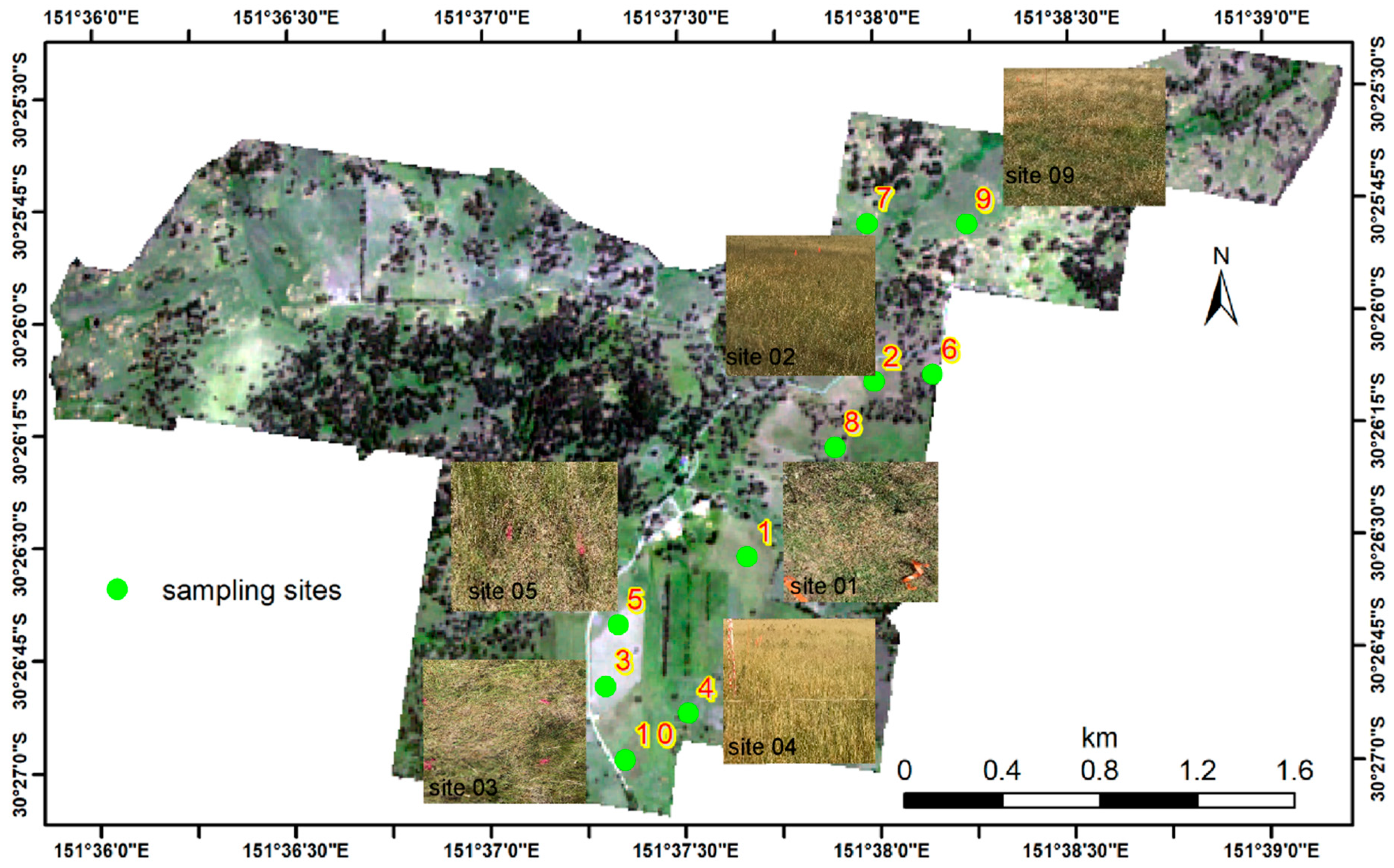
2.1. Description of Study Site and Selection of Sampling Sites

This study was conducted on one of the University of New England SMART Farms located near Armidale, NSW Australia (30°26′26″S, 151°37′30″E). The 740 ha property used is a complex pasture landscape which comprises open pasture grasslands, scattered trees, remnant vegetation communities and native forests (Figure 1). The topography ranges from undulating to hilly. The soil in the study area is predominantly Vertosols of basalt origin with Chromosols in granite areas [36]. Mean annual rainfall is 755 mm and mean annual maximum and minimum temperatures are 20.3 °C and 6.2 °C (1997–2017), respectively [37]. This study site is composed of many fields of numerous native and introduced naturalised pasture species on which grazing livestock (sheep and cattle) are rotated throughout the year. In this study, 10 different sites with a range of pasture composition, influenced by soil type and topography, were sampled (Figure 1). Each of the 10 sampling sites measured 30 m × 30 m to encapsulate the resampled (see S2.4) 10 m × 10 m spatial resolution of the S1 imagery, allowing for a 10 m radius buffer around the ‘central pixel’ location for uncertainty in spatial registration of the image pixels.

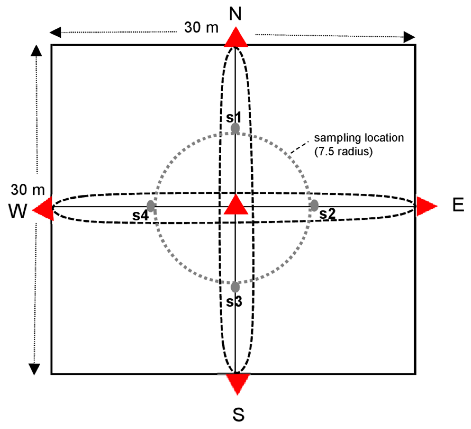
2.2. Field Data Collection and Processing

Each 30 × 30 m site was set up with the site location attributed to the centre from which the four compass direction radials (north, N; south, S; east, E; and west, W) providing transects for sampling (Figure 2). At each midway point along the four radials, AGB was sampled from a 0.5 m × 0.5 m quadrat frame resulting in forty samples from the ten sites. The sampling date (13 February 2017) was selected on account of no rainfall occurring on this date or three days beforehand, in order to limit the influence on incident radar pulse of surface moisture. While the pasture grasses were senescent and dry during sampling, many of the sites were recently grazed prior to the field measurement. The LAI was first measured using AccuPAR PAR/LAI Ceptometer followed by the pasture height using falling plate [38,39]. To assess the influence of soil moisture on the S1 polarimetry, volumetric water content of the soil, at 25 cm depth, was collected using Decagon 5TE soil sensors (Decagon Devices, Inc., 2365 NE Hopkins Court, Pullman WA, www.decagon.com) installed near the study sites. Finally, the sampled AGB was clipped to ground and the fresh AGB weighed on location. Off-field sorting to remove any foreign material was conducted, and the samples were then oven-dried at a temperature of 70 °C for at least 48 h.

2.3. Theory of Eigenvector Scattering Mechanism

The backscattering coefficient of a SAR sensor is a result of different interactions and contributions due to the sensor’s incidence angle, polarisation and frequency of operation, and the structural and dielectric properties of the sensed target [40]. The radar backscattering coefficient can, however, be de-convolved into individual scattering components, of which the dominant scattering type can be identified [41]. The eigenvector polarimetric decomposition is an eigenvalue analysis of the coherency matrix originally developed by Cloude and Pottier [42] to handle quad-polarisation data. This polarimetric decomposition technique has since evolved to utilise dual-polarisation data [43,44,45] such as the S1. In applying eigenvector decomposition to dual-polarisation data, the original formulation has been modified [46] and, as a result, a 2 × 2 coherency matrix [ C c o h ] is expressed as
[ C c o h ] = [ U ] [ λ 1 0 0 λ 2 ] [ U ] T = λ 1 u 1 u 1 T + λ 2 u 2 u 2 T
[ U ] = [ U 11 U 12 U 21 U 22 ]   = [ u 1 u 2 ] = [ cos α sin α e j δ sin a e j δ cos α ]
where λ1λ2 are eigenvalues and [ U ] is orthogonal unitary matrix while and   T represent complex conjugate and transpose matrices, respectively.
The eigenvector dual polarisation decomposition results in three roll-invariant parameters; polarimetric scattering entropy (H), scattering anisotropy (A) and the mean scattering angle (α). The H is defined as:
H = P 1   l o g 2   P 1 P 2   l o g 2 P 2
H ranges between 0–1 and when H = 0 the coherency matrix has only one eigenvalue λ1 (λ2 = 0) to imply only one scattering mechanism exists. On the contrary, H = 1 is a complete random scattering mechanism. The entropy is indicative of the number of dominant scattering mechanisms and is thus proportional to the degree of depolarisation. Anisotropy, A, provides additional information on the entropy by illustrating the contributions of secondary scattering mechanism, calculated as:
A = λ 1 λ 2 λ 1 + λ 2
The α is defined as:
α = P 1 c o s 1 ( | U 11 | ) + P 2 c o s 1 ( | U 11 | )
where
P i = λ i λ 1 + λ 2
The alpha angles of 0°, 45° and 90° represent surface scattering, dipole scattering, and double-bounce scattering mechanisms, respectively. This study explored the potential of these parameters to create a simple and interpretable regression model capable of estimating AGB.

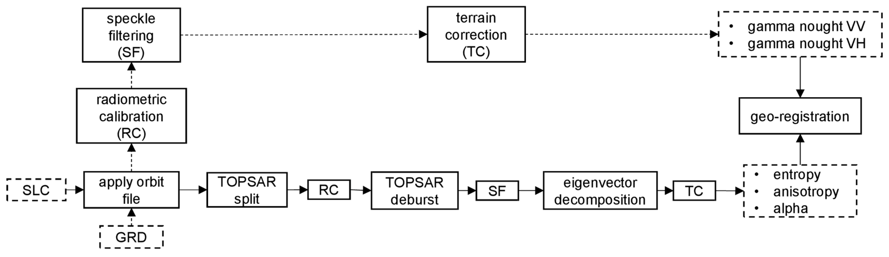
2.4. Pre-Processing of Sentinel-1 Data

Sentinel-1A interferometric wide swath data (single look complex (SLC) and ground range detected (GRD) products) with an observation date (13 February 2017) coincidental with field measurement were downloaded from the Copernicus Open Access Hub (https://scihub.copernicus.eu/dhus/#/home). Further detail of this data is reported in Table 1. This S1 data was in the dual-polarisation of VV and VH. The SLC product was processed to derive the polarimetric decomposition parameters. Firstly, the precise orbit ephemeris data from ESA archive was downloaded and applied to correct for the position of the satellite during SAR data collection [47]. Secondly, the SLC image was TOPSAR split into sub-swath 2 since this sub-swath contains our study site. Moreover, the TOPSAR split lowered image processing time, as the data file size was reduced. Additionally, the bursts of this sub-swath (due to the TOPSAR imaging technique used in S1 mission) were removed after a radiometric calibration of the image. Eigenvector polarimetric decomposition was performed using a moving window size of 3 × 3 pixels. Finally, the decomposed polarimetric product was terrain corrected using Shuttle Radar Topography Mission (SRTM) 90 m and 30 m DEMs [48] and a 1 m DEM derived from airborne LiDAR system flown over the study site in 2013 [49]. The three DEMs were used in order to evaluate the accuracy of terrain-corrected SAR images. Aside from the geometric terrain correction procedure, a nearest neighbourhood method was used to resample the image to a new spatial resolution of 10 m to match the GRD product. The radiometric calibration of the S1 GRD product was performed after the image had been corrected for satellite positional offset using the orbit state vector file. Speckle noise, due to constructive and deconstructive wave interference in the image (including the SLC image) was minimised using the Refined Lee filter method [50,51]. Finally, the GRD product was terrain corrected using the three different DEMs in a similar fashion as the SLC processing (Figure 3). The backscattering coefficients (γ°) in linear scale were converted to decibels (dB) to have these estimates in both linear and logarithmic units for further analysis. Using the backscattering coefficients in the linear scale, a volume scattering index (VSI) [52,53] was calculated as:
γ V H ° γ V H ° + γ V V °
As the depolarisation ratio has been reported in earlier studies to be sensitive to soil roughness, a suitable proxy for soil roughness [54,55] was used to assess the influence of roughness on the mean scattering angle. The depolarisation ratio is defined as the difference between cross-polarisation and co-polarisation. The SLC and GRD images were geo-registered to each other and then using a 3 × 3 pixels window size, values for all the polarimetric measures were extracted for each sampling site. All image processing was conducted in S1 Toolbox [56].

2.5. Statistical Analysis

Mean values (average of four samples per site) of the dry matter estimates of AGB were computed to achieve dry biomass estimate for each site. The mean values of LAI and pasture height were also calculated. Correlation analyses of the polarimetric parameters and field measured LAI, pasture height and AGB were conducted for the different DEMs used in processing the SAR images. In other words, the biophysical variables (LAI, height and AGB) were regressed against the VH and VV polarisations with the backscatter values in linear scale for the purposes of exploring linear, exponential, logarithmic and quadratic functions. The regression with the highest coefficient of determination (R2) was selected and reported on. Furthermore, a linear regression was conducted to investigate the significance level of the influence of soil moisture (volumetric water content) and roughness (depolarisation ratio) on the SAR signal. A generalised additive model (GAM) was built using the mean scattering angle as the only predictor. Given the univariate character of the model, a cubic regression spline was selected as the basis function for GAM [57]. The model was inspected to confirm normality of residuals and homoscedasticity using the Breusch and Pagan test [58]. Since the data for model calibration was limited in size, the GAM model was validated using a leave-one-out cross-validation (LOOCV) method as it has been assessed by earlier work to be appropriate under such constraints [59,60]. The performance of the GAM model was evaluated using adjusted R2, deviance and RMSE. All statistical analyses were conducted in R [61] with a particular use of the ‘mixed GAM computation vehicle’ (mgcv) package [62].

3. Results

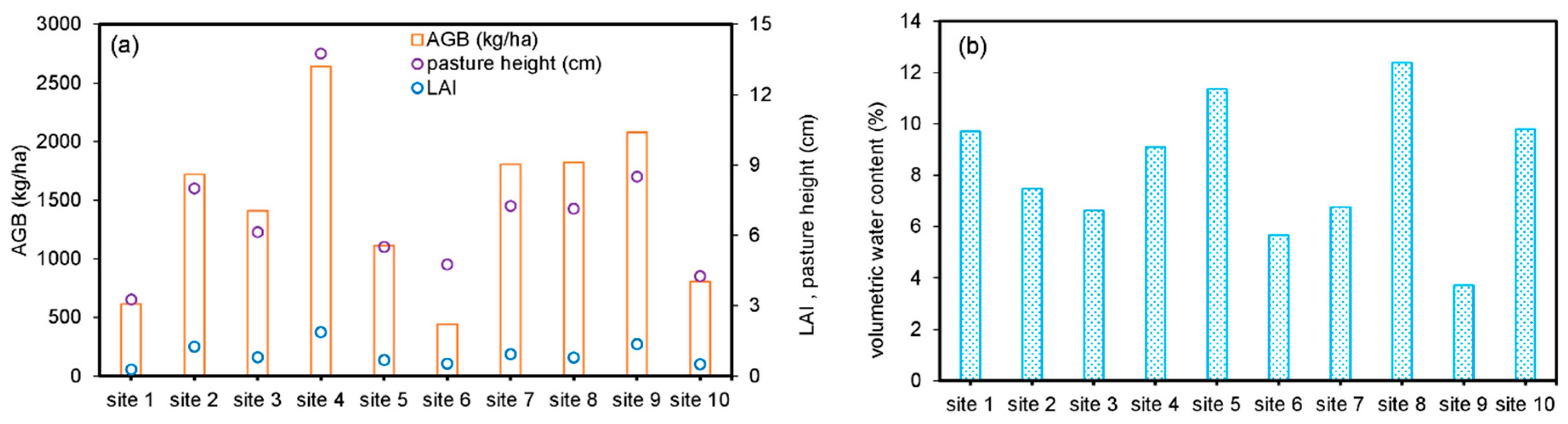
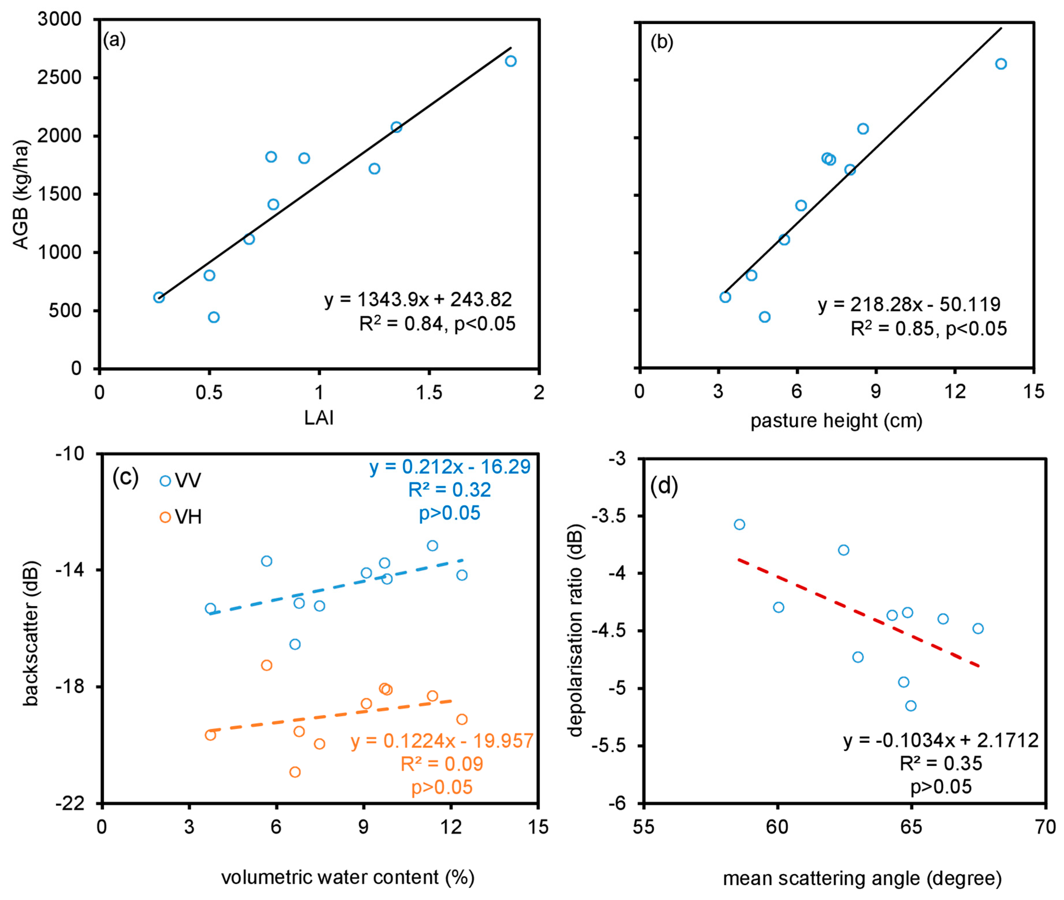
3.1. Exploratory Analysis of Field Data

The minimum pasture height and LAI values were observed in site 1 while the maximum pasture height and LAI values were observed in site 4 (Figure 4a). Moreover, the sampling site 4 recorded the highest AGB (2642 kg/ha) while the minimum AGB value (443 kg/ha) was recorded at site 6 (Figure 4a). The pasture height values range between 0.27 cm and 1.87 cm, the LAI values range between 3.25 and 13.75, while on the other hand, the AGB values varied between 614 kg/ha and 2642 kg/ha. It is worth noting that although minimum LAI and pasture height values were recorded at site 1, this site had more AGB than site 6 due to the prostrate morphology of the plant species in site 1. The inter-site soil moisture condition was characterised with the volumetric water content which ranged between 3.7% and 12.4% (Figure 4b). The minimum and maximum values of the volumetric water content were observed in site 9 and site 8, respectively. It should be noted that these values are extracted at an average depth of 25 cm. The surface moisture was rated as very low.

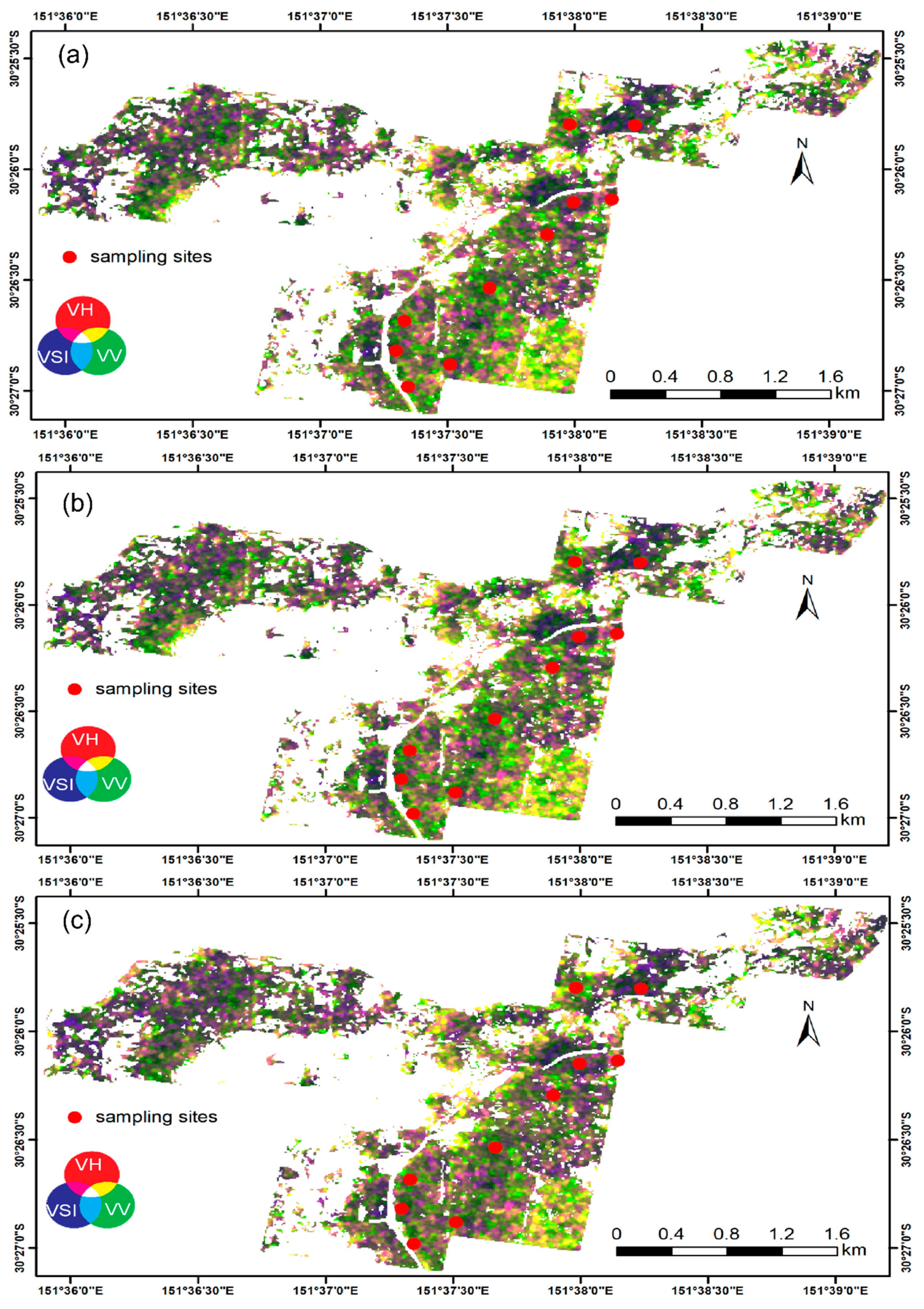
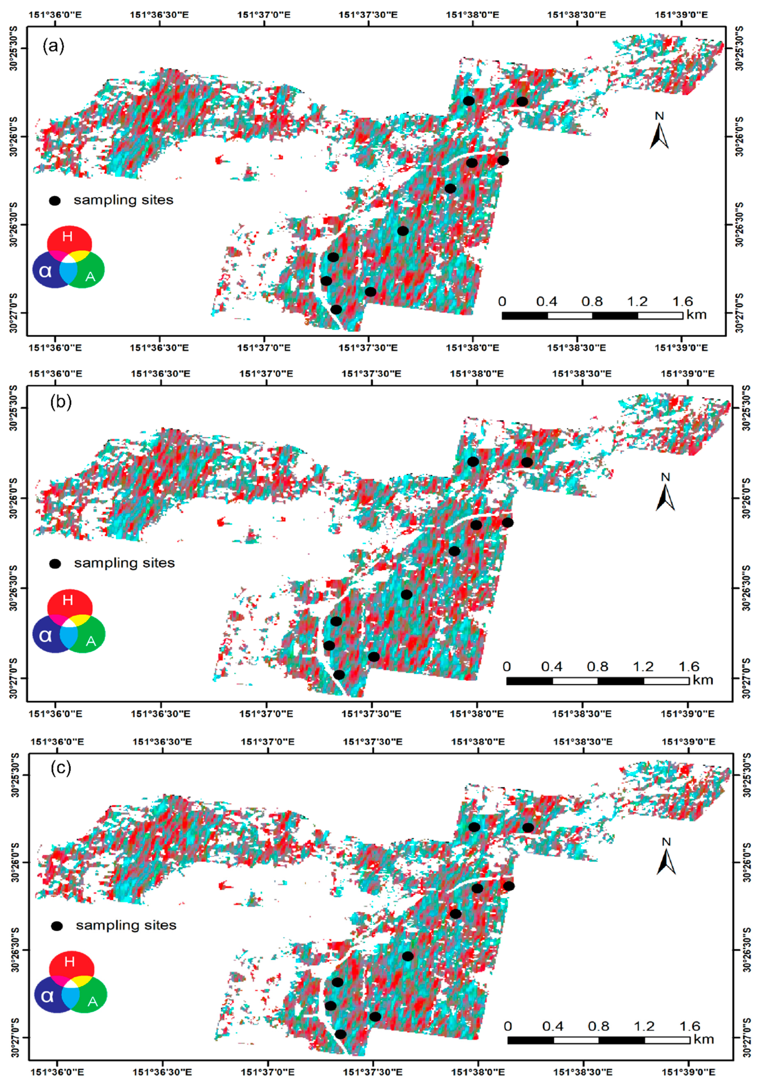
3.2. Spatial Characterisation of SAR Polarimetric Measures

Figure 5 shows the colour-coded images of the response of the pasture grasses to VH cross-polarisation (red), VV co-polarisation (green) and VSI (blue) for 90 m DEM, 30 m DEM and 1 m DEM analyses, respectively. The SAR polarisations differed according to the conditions of the pasture grass. It can be seen that the VSI, VV and the additive combination of VH and VV were pronounced in the entire study site, especially for the 1 m DEM analysis. Compared to the images for the 90 m and 30 m DEM analyses, the image for the 1 m DEM appears to show a rougher texture which suggests this analysis captures more variability of the polarimetric parameters.
Figure 6 presents colour-coded images which show the eigenvector polarimetric decomposition parameters for 90 m DEM, 30 m DEM and 1 m DEM analyses, respectively. The red, green and blue colours denote scattering entropy, scattering anisotropy and mean scattering angle, respectively. It can be seen that the entire study area is characterised with scattering entropy and the combination of scattering anisotropy and mean scattering angle.

3.3. Regression Analyses

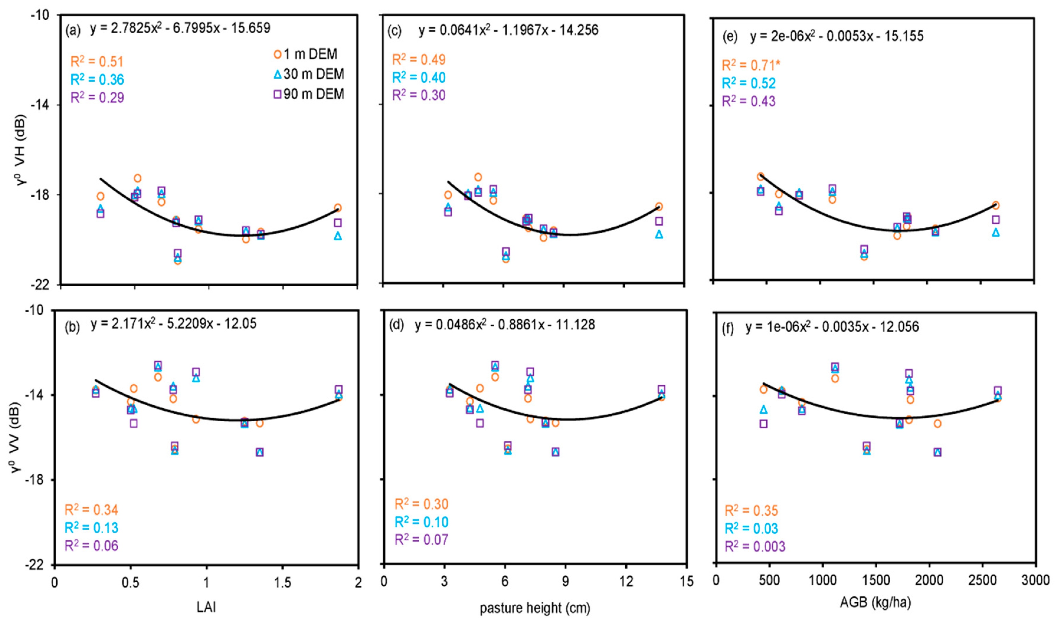
3.3.1. Field Measured Biophysical Variables and Influence of Soil Moisture and Roughness on SAR

Field measured pasture height and LAI showed strong correlations with AGB (Figure 7a,b). LAI showed a strong positive linear relationship with AGB (R2 = 0.84) as was the relationship between pasture height and AGB (R2 = 0.85). Similar results have been reported elsewhere [4].
There was no significant correlation between volumetric water content and the radar backscatter (p > 0.05), and no significant correlation existed between depolarisation ratio and the mean scattering angle (R2 = 0.35; p > 0.05) (Figure 7c,d).

3.3.2. SAR Polarisation against Biophysical Variables

Figure 8 shows the relationship between backscattering coefficients from VH and VV polarisations and LAI, pasture height and AGB for 1 m DEM, 30 m DEM and 90 m DEM-based analyses. The relationships between LAI, pasture height and AGB and both polarisations were consistently curvilinear (quadratic relation). The correlation between cross-polarisation (VH) and LAI, pasture height and AGB was consistently stronger than the correlation with co-polarisation (VV). Regarding cross-polarisation, the correlation between LAI, pasture height and AGB and backscattering coefficients for all DEM analyses varied between R2 = 0.29 to R2 = 0.71. The strongest correlation values were observed for the 1 m DEM analysis in that the LAI, pasture height and AGB measured against the backscattering coefficients produced R2 values of 0.51, 0.49 and 0.71, respectively. However, it was only the relationship between AGB and VH for the 1 m DEM anlysis that proved to be statistically significant. The convexity of the observed parabola in Figure 8e suggests lower values of AGB have an inverse linear relationship with the backscattering coefficient up until an AGB value of ~1750 kg/ha. At higher levels of AGB, the relationship is positive. For co-polarisation, the correlation values varied between R2 = 0.003 and R2 = 0.35, but none of the relationships is statistically significant. There was no statistically significant relationship observed between VSI and any of the biophysical variables.

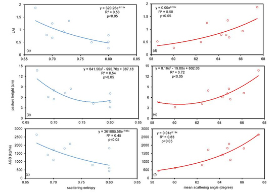
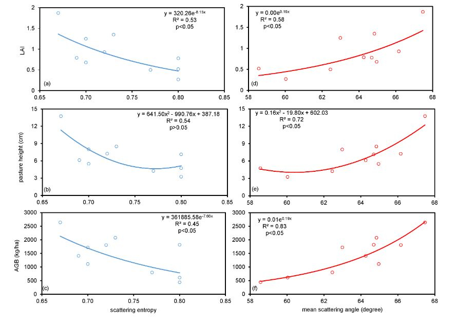
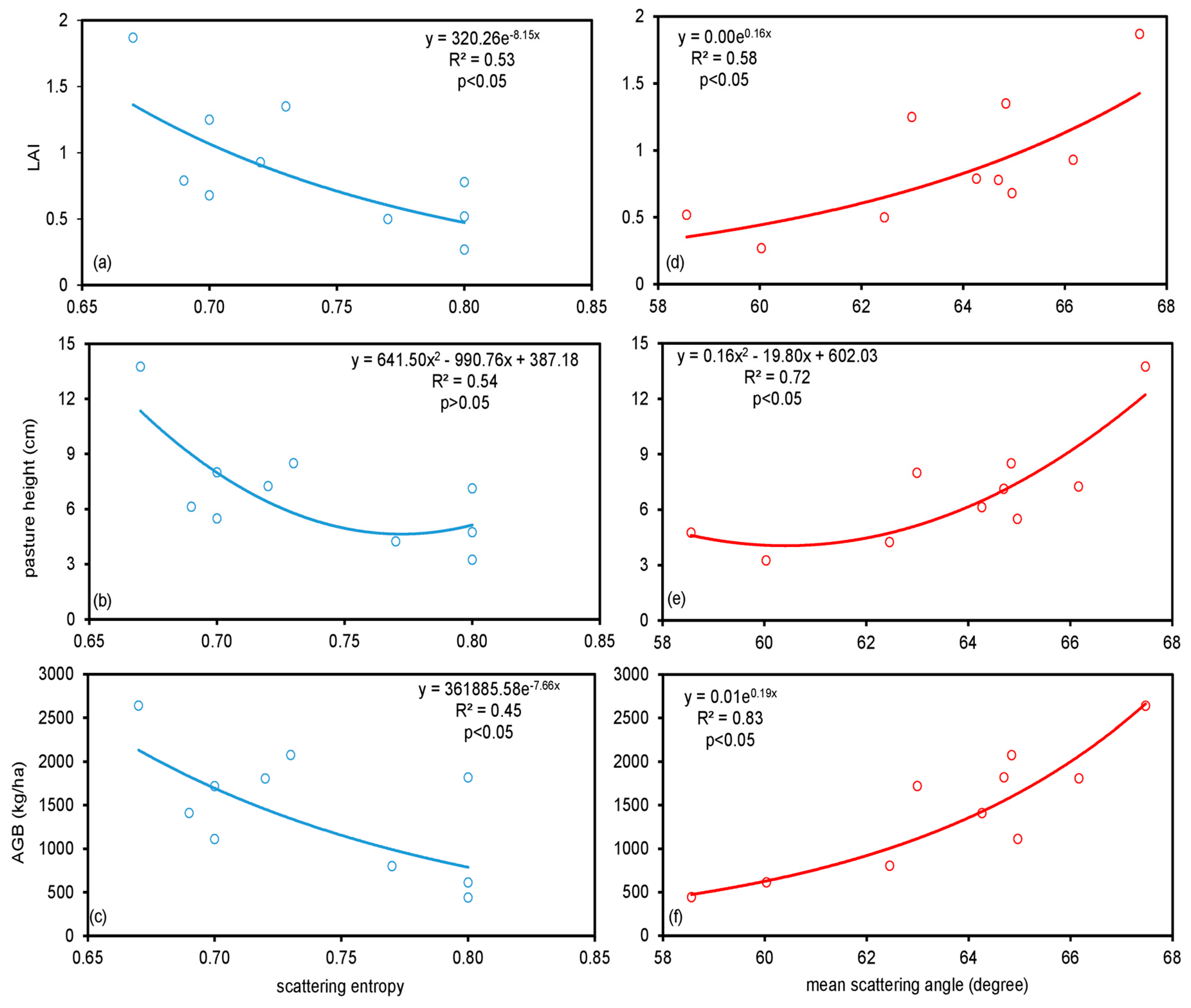
3.3.3. The Biophysical Variables against Polarimetric Scattering Parameters

Scatterplots of scattering entropy (H) and mean scattering angle (α) as a function of the biophysical variables (LAI, pasture height and AGB) are presented in Figure 9. The associated R2 values between the scattering entropy and the LAI, pasture height and AGB were 0.53, 0.54 and 0.45, respectively (Figure 9a–c). The R2 values associated with mean scattering angle and the LAI, pasture height and AGB were 0.58, 0.72 and 0.83, respectively. The relationships between these polarimetric measures and the biophysical variables were exponential or quadratic and with exception of pasture height, were monotonically decreasing (scattering entropy) or increasing (mean scattering angle) with increasing parameter values. There were significant relationships between the scattering entropy and LAI and AGB only (p < 0.05). On the other hand, the relationships between mean scattering angle and all the biophysical variables were statistically significant.

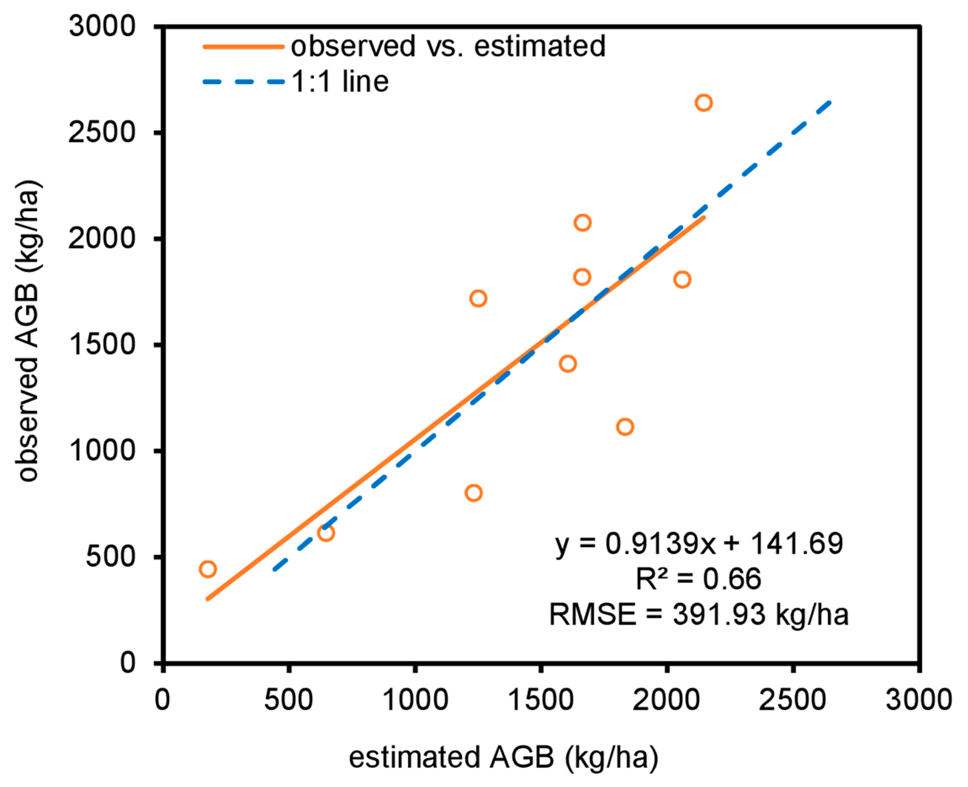
3.4. Generalised Additive Model for AGB Estimation

A statistically significant, generalised additive model (GAM) for AGB estimation was created using the mean scattering angle (α) (Table 2). A post-model Breusch-Pagan analysis produced a test statistic of 0.336, implying a constant variance of the model, producing an RMSE of 391.93 kg/ha for AGB values that ranged between 443 kg/ha and 2642 kg/ha (Figure 10).

4. Discussion

4.1. The Influence of Topography on SAR Measures

The spatial resolution of the DEM played a significant role in the ability of S1 derived metrics to explain the variance observed in the biophysical variables at the field sites. Only when incorporating the 1 m DEM did the S1 metrics provide a statistically significant explanation of the variability in pasture AGB (Figure 8e). This finding is similar to Hinse et al. [25] who showed that DEM products of higher spatial resolution than the SRTM 30 m DEM captured more backscatter variations in a SAR image. Similarly, Ortiz et al. [29] reported that, compared to the traditional SRTM DEM (90 m), a DEM of 5 m spatial resolution minimised errors in pixel location and prediction of forest types. As with the field sites examined in this work, the effects of significant topographic variations can be mitigated with higher spatial resolution DEMs because errors in scattering mechanisms associated with terrain slope in azimuth and range directions are minimised [27,30,63].

4.2. Relationship between the Biophysical Variables and Polarimetric SAR Parameters

Compared to VH cross-polarisation, the backscatter values for the VV co-polarisation were higher and this could be attributed to the predominantly vertical (erectophile) canopy of the grass blades oriented parallel to the electrical field vector of the incident microwave energy [64,65]. Similarly, surface scattering from the exposed soil and detached (horizontal) pasture components resulting from grazing could account for the high backscatter values for the VV co-polarisation. Whilst the VV polarisation is also noted to be more sensitive to soil moisture, the conditions at the field site at the time of data collection were such that surface moisture was considered negligible.
The aboveground pasture biomass, whilst a quantitative measure of pasture amount of importance to pasture managers, from a radar sensor perspective, is effectively the integration of gross morphological characteristics such as LAI, leaf orientation (predominantly erectophile) and canopy height. The only statistically significant relationship between S1 parameters and AGB was observed with VH (1 m DEM analysis), and this is consistent with previous studies where cross-polarised channels were observed to be more responsive to variation in AGB than co-polarised channels [34,40,66]. The quadratic relationship observed between VH and AGB is likely the result of two interacting phenomena. At lower AGB values which were recorded in more heavily grazed sites, the grazing activity exposes the underlying soil and thus the relative high backscattering coefficient could be attributed to surface roughness contributions. At higher AGB the contribution of volume or multiple scattering from the grass canopy to the backscattering coefficient dominates. The curves suggest the switch from surface to canopy-dominance in the S1 response occurs at approximately 1750 kg/ha (Figure 8), coinciding with a, LAI of ~1.3 and a pasture height of ~10 cm. This is consistent with the canopy peneration limits noted in other work [18,19]. On the other hand, the polarimetric scattering was highly random given the dominance of the entropy and anisotropy (in combination with the alpha) (Figure 6).
A non-linear relationship was observed between the LAI, pasture height and AGB and the polarimetric scattering parameters (entropy and alpha) (Figure 9). Particularly, significant relationships were observed between scattering entropy and LAI and AGB while the relationships between the mean scattering angle (α) and all the biophysical variables (LAI, pasture height and AGB) were significant. This suggests that the LAI and AGB were more strongly driving the S1 response. Given the similarity in the relationship between all the biophysical variables (LAI, pasture height and AGB) and the polarimetric scattering parameters, the discussion is focused on only the LAI. The LAI estimates decay with increasing scattering entropy to explain the influence of grazing on return backscattering signal. Since the leaf area is reduced by grazing, the exposed rough surface and lower pasture height with different leaf orientations are likely to subject incident microwave energy to many scattering events before reaching the receiving antenna. In other words, the sites with low LAI values minimise the contributions of volume scatterers. Conversely, the LAI estimates grow with increasing mean scattering angle. This observation is likely to be caused by a more active volume scattering at sites with denser canopies.

4.3. Estimation of Pasture Grass AGB

The GAM model offered a significant intercept term which estimated the overall mean AGB at 1445.3 kg/ha (±115.5 as standard error). An estimated degree of freedom of 1 implies the near-approximation of the GAM model to a linear function. Meanwhile, the smoothing function applied in the GAM to explain the non-linear relationship between AGB and mean scattering angle was statistically significant (p-value < 0.05). The GAM model explained 75.7% of deviance in the AGB observations and a comparison of the observed versus GAM-estimated AGB yielded an RMSE of 391.93 kg/ha (R2 = 0.66) (Figure 10). Such a result should be interpreted with caution given the sparsity of data and the consequent use of a leave one out cross validation process instead of separate calibration and validation datasets. Moreover, the data were collected in just a single season which does not enable conclusions to be made around seasonal translatability. However, the results of this preliminary investigation are encouraging given the fact that the S1 system is satellite based and offers advantages over optical satellite systems such as ability to collect data under observation conditions that preclude the use of optical satellite sensors. The use of comparable spatial resolution optical systems such as Landsat TM and SPOT XS which have been observed to yield pasture biomass estimations with an RMSE of 315 kg DM/ha [8] could be augmented through the use of radar systems such as S1, not only if/when constrained by target visibility but also when the target comprises of senesced grasses which is typically beyond the sensitivity of pigment-based, spectro-optical indices such as the NDVI.
The accuracy of the GAM model in this study is consistent with past studies that estimated AGB using near-surface optical remote sensing devices or satellite-based SAR polarimetric variables. For similar study sites in Australia, the RMSE of 391.93 kg/ha observed in this study compares with the 288 kg/ha and 537 kg/ha prediction errors reported by Trotter et al. [6] and Andersson et al. [4], respectively, using proximal active optical sensors. Moreover, the accuracy of the present AGB model compares with the accuracy (RMSE of 455.28 kg/ha) reported in Schaefer and Lamb [5] who used terrestrial LiDAR system. Regarding similar past SAR studies, the accuracy of this GAM model is comparable to the RMSE of 511 kg/ha produced by a linear regression model created on the difference in backscattering coefficients of VV and VH polarisation of TerraSAR-X [33].
In addition to the qualifiers around limited data and single season data capture mentioned earlier, the use of sites with low LAI or pasture heights limits the interaction between canopy scatterers and transmitted radar signal, and this has limited the ability of the volume scattering process to capture the variability of the LAI, pasture height and hence, the AGB. The eigenvector polarimetric parameters suggest the dominance of volume scattering and surface scattering mechanisms, but this present study was unable to separate and analyse these mechanisms individually. In future work, full polarimetric data and a larger range of canopy conditions (LAI, height) will be included to permit the use of other polarimetric decomposition methods such as Freeman-Durden [67] to evaluate the individual scattering mechanisms. However it should be noted that the constraints experienced in this present work were realistic, operational constraints that may typically occur in any real farming enterprise (i.e., grazing pressure, biomass range restrictions to promote sustainable pasture regeneration in the light of maintaining livestock carrying capacity, impacts of drought etc.) and so the applicability of such ‘enhanced’ datasets to the ‘real world’ should be carefully considered.

5. Conclusions

The response of a range of Sentinel-1 (S1) backscatter parameters to the biophysical characteristics of native pasture grasses including leaf area index, pasture height and aboveground biomass were investigated in the context of a hilly, pastoral farm. The S1 parameters included VH cross-polarisation and VV co-polarisation as well as derived metrics including volume scattering index and eigenvector polarimetric decomposition parameters (entropy, anisotropy and alpha). Analyses involved the use of digital elevation models of varying spatial resolutions; 90 m, 30 m and 1 m. Owing to the enhanced ability of the highest-resolution, 1 m DEM data, to capture the terrain/topographic induced errors in backscatter parameter analysis, the 1 m DEM-based analysis produced the highest accuracies in explaining the relationships between the biophysical variables and Sentinel-1 polarimetric features. This observation reinforces the value of high-resolution DEM data for analysing signals emanating from landscapes with significant topographic variability. A generalised additive model with mean scattering angle as a predictor was established to estimate aboveground pasture biomass. The root mean square error of prediction for the model was 391.93 kg/ha over a biomass range of 443–2642 kg/ha with pasture LAI ranging from 0.27 to 1.87 and height 3.25 cm to 13.75 cm. Whilst only a preliminary investigation limited by sparse data and a single season of data capture, the results are encouraging and should motivate further investigations for using S1 to assess pasture biomass, especially under conditions of significant senescence and where spatial scale precludes the use of on-ground measurement techniques. Certainly, further work is required to investigate seasonality and transferability across multiple seasons. Additionally, this study should encourage further investigations into augmenting existing optical sensor-based systems, for example the ‘Pastures from Space’ programme in Australia and New Zealand.

Author Contributions

Conceptualization, R.A.C. and D.W.L.; Formal analysis, R.A.C.; Investigation, R.A.C., C.E., K.A. and D.S.; Methodology, R.A.C. and D.W.L.; Supervision, D.W.L.; Writing—original draft, R.A.C.; Writing—review & editing, D.W.L., C.E., K.A. and D.S.

Funding

This research received no external funding.

Acknowledgments

The first author acknowledges receipt of a Tuition Fee Scholarship from the University of New England. Food Agility CRC Ltd. is funded under the Commonwealth Government CRC Program. The CRC Program supports industry-led collaborations between industry, researchers and the community. All authors gratefully acknowledge the contribution of Joshua Stover (from the UNE-PARG) for his useful comments.

Conflicts of Interest

The authors declare no conflict of interest.

References

  1. Behrendt, K.; Cacho, O.; Scott, J.M.; Jones, R. Optimising pasture and grazing management decisions on the Cicerone Project farmlets over variable time horizons. Anim. Prod. Sci. 2013, 53, 796. [Google Scholar] [CrossRef]
  2. Gherardi, S.; Anderton, L.; Sneddon, J.; Oldham, C.; Mata, G. Pastures from space–the value to Australian sheep producers of satellite-based pasture information. In Proceedings of the 12th Australasian Remote Sensing and Photogrammetry Conference, Freemantle, WA, Australia, 18–22 October 2004. [Google Scholar]
  3. Hanrahan, L.; Geoghegan, A.; O’Donovan, M.; Griffith, V.; Ruelle, E.; Wallace, M.; Shalloo, L. PastureBase Ireland: A grassland decision support system and national database. Comput. Electron. Agric. 2017, 136, 193–201. [Google Scholar] [CrossRef]
  4. Andersson, K.; Trotter, M.; Robson, A.; Schneider, D.; Frizell, L.; Saint, A.; Lamb, D.; Blore, C. Estimating pasture biomass with active optical sensors. Adv. Anim. Biosci. 2017, 8, 754–757. [Google Scholar] [CrossRef]
  5. Schaefer, M.T.; Lamb, D.W. A combination of plant NDVI and LiDAR measurements improve the estimation of pasture biomass in tall fescue (Festuca arundinacea var. Fletcher). Remote Sens. 2016, 8, 109. [Google Scholar] [CrossRef]
  6. Trotter, M.; Lamb, D.; Donald, G.; Schneider, D. Evaluating an active optical sensor for quantifying and mapping green herbage mass and growth in a perennial grass pasture. Crop Pasture Sci. 2010, 61, 389–398. [Google Scholar] [CrossRef]
  7. Clarke, D.; Litherland, A.; Mata, G.; Burling-Claridge, R. Pasture Monitoring from Space. In Proceedings of the South Island Dairy Event Conference, Invercargill, New Zealand, 26–28 June 2006; pp. 108–123. [Google Scholar]
  8. Edirisinghe, A.; Hill, M.J.; Donald, G.E.; Hyder, M. Quantitative mapping of pasture biomass using satellite imagery. Int. J. Remote Sens. 2011, 32, 2699–2724. [Google Scholar] [CrossRef]
  9. Barrachina, M.; Cristóbal, J.; Tulla, A.F. Estimating above-ground biomass on mountain meadows and pastures through remote sensing. Int. J. Appl. Earth Obs. Geoinf. 2015, 38, 184–192. [Google Scholar] [CrossRef]
  10. Sibanda, M.; Mutanga, O.; Rouget, M.; Kumar, L. Estimating biomass of native grass grown under complex management treatments using WorldView-3 spectral derivatives. Remote Sens. 2017, 9, 55. [Google Scholar] [CrossRef]
  11. Ramoelo, A.; Cho, M.A.; Mathieu, R.; Madonsela, S.; van de Kerchove, R.; Kaszta, Z.; Wolff, E. Monitoring grass nutrients and biomass as indicators of rangeland quality and quantity using random forest modelling and WorldView-2 data. Int. J. Appl. Earth Obs. Geoinf. 2015, 43, 43–54. [Google Scholar] [CrossRef]
  12. Lamb, D.W.; Steyn-Ross, M.; Schaare, P.; Hanna, M.M.; Silvester, W.; Steyn-Ross, A. Estimating leaf nitrogen concentration in ryegrass (Lolium spp.) pasture using the chlorophyll red-edge: theoretical modelling and experimental observations. Int. J. Remote Sens. 2002, 23, 3619–3648. [Google Scholar] [CrossRef]
  13. Prabhakara, K.; Hively, W.D.; McCarty, G.W. Evaluating the relationship between biomass, percent groundcover and remote sensing indices across six winter cover crop fields in Maryland, United States. Int. J. Appl. Earth Obs. Geoinf. 2015, 39, 88–102. [Google Scholar] [CrossRef] [Green Version]
  14. Asrar, G.; Fuchs, M.; Kanemasu, E.; Hatfield, J. Estimating Absorbed Photosynthetic Radiation and Leaf Area Index from Spectral Reflectance in Wheat 1. Agron. J. 1984, 76, 300–306. [Google Scholar] [CrossRef]
  15. Gallo, K.P.; Daughtry, C.S.T. Techniques for Measuring Intercepted and Absorbed Photosynthetically Active Radiation in Corn Canopies 1. Agron. J. 1986, 78, 752–756. [Google Scholar] [CrossRef]
  16. Carver, K.R.; Elachi, C.; Ulaby, F.T. Microwave remote sensing from space. Proc. IEEE 1985, 73, 970–996. [Google Scholar] [CrossRef] [Green Version]
  17. Moreira, A.; Prats-Iraola, P.; Younis, M.; Krieger, G.; Hajnsek, I.; Papathanassiou, K.P. A tutorial on synthetic aperture radar. IEEE Geosci. Remote Sens. Mag. 2013, 1, 6–43. [Google Scholar] [CrossRef] [Green Version]
  18. Ghasemi, N.; Sahebi, M.R.; Mohammadzadeh, A. A review on biomass estimation methods using synthetic aperture radar data. Int. J. Geomat. Geosci. 2011, 1, 13. [Google Scholar]
  19. Wang, X.; Ge, L.; Li, X. Pasture Monitoring Using SAR with COSMO-SkyMed, ENVISAT ASAR, and ALOS PALSAR in Otway, Australia. Remote Sens. 2013, 5, 3611–3636. [Google Scholar] [CrossRef] [Green Version]
  20. Saatchi, S.S.; van Zyl, J.J.; Asrar, G. Estimation of canopy water content in Konza Prairie grasslands using synthetic aperture radar measurements during FIFE. J. Geophys. Res. 1995, 100, 25481. [Google Scholar] [CrossRef]
  21. Bouman, B.A.M.; van Kasteren, H.W.J. Ground-based X-band (3-cm wave) radar backscattering of agricultural crops. II. Wheat, barley, and oats; the impact of canopy structure. Remote Sens. Environ. 1990, 34, 107–119. [Google Scholar] [CrossRef]
  22. Haldar, D.; Chakraborty, M.; Manjunath, K.R.; Parihar, J.S. Role of Polarimetric SAR data for discrimination/biophysical parameters of crops based on canopy architecture. ISPRS-Int. Arch. Photogramm. Remote Sens. Spat. Inf. Sci. 2014, XL–8, 737–744. [Google Scholar] [CrossRef]
  23. Franklin, S.; Lavigne, M.; Hunt, E., Jr.; Wilson, B.; Peddle, D.; McDermid, G.; Giles, P. Topographic dependence of synthetic aperture radar imagery. Comput. Geosci. 1995, 21, 521–532. [Google Scholar] [CrossRef]
  24. Goyal, S.K.; Seyfried, M.S.; O’Neill, P.E. Effect of digital elevation model on topographic correction of airborne SAR. Int. J. Remote Sens. 1998, 19, 3075–3096. [Google Scholar] [CrossRef]
  25. Hinse, M.; Gwyn, Q.; Bonn, F. Radiometric correction of C-band imagery for topographic effects in regions of moderate relief. IEEE Trans. Geosci. Remote Sens. 1988, 26, 122–132. [Google Scholar] [CrossRef]
  26. Leclerc, G.; Beaulieu, N.; Bonn, F. A simple method to account for topography in the radiometric correction of radar imagery. Int. J. Remote Sens. 2001, 22, 3553–3570. [Google Scholar] [CrossRef] [Green Version]
  27. Small, D. Flattening gamma: Radiometric terrain correction for SAR imagery. IEEE Trans. Geosci. Remote Sens. 2011, 49, 3081–3093. [Google Scholar] [CrossRef]
  28. Van Zyl, J.J.; Chapman, B.D.; Dubois, P.; Shi, J. The effect of topography on SAR calibration. IEEE Trans. Geosci. Remote Sens. 1993, 31, 1036–1043. [Google Scholar] [CrossRef]
  29. Ortiz, S.M.; Breidenbach, J.; Knuth, R.; Kändler, G. The influence of DEM quality on mapping accuracy of coniferous- and deciduous-dominated forest using TerraSAR-X images. Remote Sens. 2012, 4, 661–681. [Google Scholar] [CrossRef]
  30. Shimada, M. Orthorectification and slope correction of SAR data using DEM and its accuracy evaluation. IEEE J. Sel. Top. Appl. Earth Obs. Remote Sens. 2010, 3, 657–671. [Google Scholar] [CrossRef]
  31. Toutin, T. Geometric processing of remote sensing images: models, algorithms and methods. Int. J. Remote Sens. 2004, 25, 1893–1924. [Google Scholar] [CrossRef]
  32. Shimada, M.; Ohtaki, T. Generating large-scale high-quality SAR mosaic datasets: application to PALSAR Data for global monitoring. IEEE J. Sel. Top. Appl. Earth Obs. Remote Sens. 2010, 3, 637–656. [Google Scholar] [CrossRef]
  33. McNeill, S.J.; Pairman, D.; Belliss, S.E.; Dalley, D.; Dynes, R. Robust Estimation of Pasture Biomass Using Dual-polarisation TerrASAR-X Imagery; IEEE: Piscataway, NJ, USA, 2010; pp. 3094–3097. [Google Scholar]
  34. Li, Z.; Guo, X. Can polarimetric RADARSAT-2 images provide a solution to quantify non-photosynthetic vegetation biomass in semi-arid mixed grassland? Can. J. Remote Sens. 2017, 43, 593–607. [Google Scholar] [CrossRef]
  35. ESA, Sentinel-1 Team Sentinel-1 User Handbook 2013. Available online: https://sentinel.esa.int (accessed on 3 May 2017).
  36. Isbell, R. The Australian Soil Classification; CSIRO Publishing: Clayton, Australia, 2016; ISBN 1-4863-0464-8. [Google Scholar]
  37. BoM Climate statistics for Australian locations. Available online: http://www.bom.gov.au/climate/averages/tables/cw_056037_All.shtml (accessed on 21 October 2018).
  38. Oliveira, D.; Medeiros, S.; Aroeira, L.; Barioni, L.; Lana, D. Estimating herbage mass in stargrass (Cynodon nlenfuensis var nlenfuensis) using sward surface height and the rising plate meter. In Proceedings of the XIX International Grassland Congress: Grassland Ecosystems: An outlook into the 21st century, Sao Pedro, Brazil, 11–21 February 2001; pp. 1055–1056. [Google Scholar]
  39. Scrivner, J.H.; Center, D.M.; Jones, M.B. A rising plate meter for estimating production and utilization. J. Range Manag. 1986, 39, 475–477. [Google Scholar] [CrossRef]
  40. Le Toan, T.; Beaudoin, A.; Riom, J.; Guyon, D. Relating forest biomass to SAR data. IEEE Trans. Geosci. Remote Sens. 1992, 30, 403–411. [Google Scholar] [CrossRef]
  41. Cloude, S.R.; Pottier, E. A review of target decomposition theorems in radar polarimetry. IEEE Trans. Geosci. Remote Sens. 1996, 34, 498–518. [Google Scholar] [CrossRef]
  42. Cloude, S.R.; Pottier, E. An entropy based classification scheme for land applications of polarimetric SAR. IEEE Trans. Geosci. Remote Sens. 1997, 35, 68–78. [Google Scholar] [CrossRef]
  43. Cloude, S. The Dual Polarization Entropy/Alpha Decomposition: A PALSAR Case Study. In Proceedings of the 3rd International Workshop on Science and Applications of SAR Polarimetry and Polarimetric Interferometry Conference, Frascati, Italy, January 22–26 2007; Volume 2. [Google Scholar]
  44. Ghods, S.; Shojaedini, S.V.; Maghsoudi, Y. A Modified H−α Classification Method for DCP Compact Polarimetric Mode by Reconstructing Quad H and α Parameters From Dual Ones. IEEE J. Sel. Top. Appl. Earth Obs. Remote Sens. 2016, 9, 2233–2241. [Google Scholar] [CrossRef]
  45. Ji, K.; Wu, Y. Scattering Mechanism Extraction by a Modified Cloude-Pottier Decomposition for Dual Polarization SAR. Remote Sens. 2015, 7, 7447–7470. [Google Scholar] [CrossRef] [Green Version]
  46. Lee, J.-S.; Pottier, E. Polarimetric Radar Imaging: From Basics to Applications; Optical Science and Engineering; CRC Press: Boca Raton, FL, USA, 2009; ISBN 978-1-4200-5497-2. [Google Scholar]
  47. Peter, H.; Jäggi, A.; Fernández, J.; Escobar, D.; Ayuga, F.; Arnold, D.; Wermuth, M.; Hackel, S.; Otten, M.; Simons, W.; et al. Sentinel-1A–First precise orbit determination results. Adv. Space Res. 2017, 60, 879–892. [Google Scholar] [CrossRef]
  48. Yang, L.; Meng, X.; Zhang, X. SRTM DEM and its application advances. Int. J. Remote Sens. 2011, 32, 3875–3896. [Google Scholar] [CrossRef]
  49. Verma, N.; Lamb, D.; Reid, N.; Wilson, B. Comparison of Canopy Volume Measurements of Scattered Eucalypt Farm Trees Derived from High Spatial Resolution Imagery and LiDAR. Remote Sens. 2016, 8, 388. [Google Scholar] [CrossRef]
  50. Lee, J.-S. Refined filtering of image noise using local statistics. Comput. Graph. Image Process. 1981, 15, 380–389. [Google Scholar] [CrossRef] [Green Version]
  51. Yommy, A.S.; Liu, R.; Wu, A.S. SAR Image Despeckling Using Refined Lee Filter. In Proceedings of the 2015 7th International Conference on Intelligent Human-Machine Systems and Cybernetics, Hangzhou, China, 26–27 August 2015; Volume 2, pp. 260–265. [Google Scholar]
  52. Parisi, J.F.; Ustin, S.L. Quantitative estimation of standing biomass from L-band multipolarization data. In Proceedings of the 10th Annual International Symposium on Geoscience and Remote Sensing, College Park, MD, USA, 15–18 May 1990; pp. 147–150. [Google Scholar]
  53. Pope, K.O.; Rey-Benayas, J.M.; Paris, J.F. Radar remote sensing of forest and wetland ecosystems in the Central American tropics. Remote Sens. Environ. 1994, 48, 205–219. [Google Scholar] [CrossRef]
  54. Oh, Y.; Sarabandi, K.; Ulaby, F.T. An empirical model and an inversion technique for radar scattering from bare soil surfaces. IEEE Trans. Geosci. Remote Sens. 1992, 30, 370–381. [Google Scholar] [CrossRef]
  55. Srivastava, H.S.; Patel, P.; Navalgund, R.R.; Sharma, Y. Retrieval of surface roughness using multi-polarized Envisat-1 ASAR data. Geocarto Int. 2008, 23, 67–77. [Google Scholar] [CrossRef]
  56. Veci, L.; Prats-Iraola, P.; Scheiber, R.; Collard, F.; Fomferra, N.; Engdahl, M. The Sentinel-1 Toolbox; 2014. In Proceedings of the IEEE International Geoscience and Remote Sensing Symposium, Quebec, QC, Canada, 14–18 July 2012; pp. 1–3. [Google Scholar]
  57. Yee, T.W.; Mitchell, N.D. Generalized additive models in plant ecology. J. Veg. Sci. 1991, 2, 587–602. [Google Scholar] [CrossRef]
  58. Breusch, T.S.; Pagan, A.R. A simple test for heteroscedasticity and random coefficient variation. Econom. J. Econom. Soc. 1979, 1287–1294. [Google Scholar] [CrossRef]
  59. Domingo, D.; Lamelas-Gracia, M.T.; Montealegre-Gracia, A.L.; Riva-Fernández, J. de la Comparison of regression models to estimate biomass losses and CO2 emissions using low-density airborne laser scanning data in a burnt Aleppo pine forest. Eur. J. Remote Sens. 2017, 50, 384–396. [Google Scholar] [CrossRef]
  60. Meng, B.; Ge, J.; Liang, T.; Yang, S.; Gao, J.; Feng, Q.; Cui, X.; Huang, X.; Xie, H. Evaluation of Remote Sensing Inversion Error for the Above-Ground Biomass of Alpine Meadow Grassland Based on Multi-Source Satellite Data. Remote Sens. 2017, 9, 372. [Google Scholar] [CrossRef]
  61. R Core Team, R: A Language and Environment for Statistical Computing; R Foundation for Statistical Computing: Vienna, Austria, 2018.
  62. Wood, S.N.; Pya, N.; Säfken, B. Smoothing Parameter and Model Selection for General Smooth Models. J. Am. Stat. Assoc. 2016, 111, 1548–1563. [Google Scholar] [CrossRef]
  63. Ulander, L.M.H. Radiometric slope correction of synthetic-aperture radar images. IEEE Trans. Geosci. Remote Sens. 1996, 34, 1115–1122. [Google Scholar] [CrossRef]
  64. Henderson, F.M.; Lewis, A.J. Principles and Applications of Imaging Radar. Manual of Remote Sensing, 3rd ed.; John Wiley & Sons: New York, NY, USA, 1998; Volume 2. [Google Scholar]
  65. Patel, P.; Srivastava, H.S.; Panigrahy, S.; Parihar, J.S. Comparative evaluation of the sensitivity of multi-polarized multi-frequency SAR backscatter to plant density. Int. J. Remote Sens. 2006, 27, 293–305. [Google Scholar] [CrossRef]
  66. Luckman, A.; Baker, J.; Kuplich, T.M.; da Costa Freitas Yanasse, C.; Frery, A.C. A study of the relationship between radar backscatter and regenerating tropical forest biomass for spaceborne SAR instruments. Remote Sens. Environ. 1997, 60, 1–13. [Google Scholar] [CrossRef]
  67. Freeman, A.; Durden, S.L. Three-component scattering model to describe polarimetric SAR data. In Proceedings of the Radar Polarimetry, San Diego, CA, USA, 12 February 1993; Volume 1748, pp. 213–225. [Google Scholar]
Figure 1. True colour (RGB) Sentinel-2A image (24 February 2017 acquisition) of study site with some photo insets, and the central location point of the ten sampling sites (indicated by green circles and are not drawn to scale). Each sampling site was 900 m2.
Remotesensing 11 00872 g001
Figure 2. Field sampling set up. The red triangles are demarcations for site central position and transect radii (North, East, South, and West). The grey dots are mid-positions of transect radii from the site’s central location and provide sampling locations (s1, s2, s3 and s4).
Remotesensing 11 00872 g002
Figure 3. The work flow for Sentinel-1 image processing. The broken rectangles represent input or output data. The input data are single look complex (SLC) and ground range detected (GRD). The solid rectangles depict the processes conducted, the solid connected arrows indicate the processing steps for SLC while broken arrows connect processes performed over GRD. The output data for SLC were polarimetric scattering entropy, scattering anisotropy and mean scattering alpha angle while that of the GRD are backscattering coefficients in gamma nought for both polarisations.
Remotesensing 11 00872 g003
Figure 4. The field measured; (a) leaf area index (LAI), pasture height and aboveground biomass (AGB) and (b) volumetric water content for each site.
Remotesensing 11 00872 g004
Figure 5. True colour composite images for backscattering coefficients processed with digital elevation model of varied spatial resolutions; (a) 90 m, (b) 30 m and (c) 1 m. The red colour in the image denotes the VH cross-polarisation, the green colour denotes the VV co-polarisation while the blue colour represents the volume scattering index (VSI). The image is the study site without non-herbaceous land cover types. Pixels in white colour represent masked land cover types or image background.
Remotesensing 11 00872 g005
Figure 6. True colour composite images for polarimetric decomposition parameters. The images represent scattering entropy (H), scattering anisotropy (A) and mean scattering angle (α) processed with digital elevation model (DEM) of varied spatial resolutions; (a) 90 m, (b) 30 m and (c) 1 m. The red colour in the image denotes the scattering entropy, green colour denotes the scattering anisotropy while blue colour represents the mean scattering angle. Areas with non-herbaceous land cover types have been masked from the image (pixels in white colour represent masked land cover types or image background).
Remotesensing 11 00872 g006
Figure 7. Correlation between: (a,b) leaf area index (LAI), pasture height and aboveground biomass (AGB), (c) volumetric water content and backscattering coefficients, and (d) mean scattering angle and depolarisation ratio.
Remotesensing 11 00872 g007
Figure 8. Relationship between the VH cross-polarisation and VV co-polarisation and biophysical variables; (a,b) leaf area index, (c,d) pasture height and (e,f) aboveground biomass. The parabola is a representation of the relationships observed for the 1 m DEM analysis only. The parabolas for 30 m and 90 m DEM analyses were not shown to preserve clarity of figures. The R2 values are for the 1 m, 30 m and 90 m DEM analyses, respectively. * denotes significant relationship at 95% confidence level.
Remotesensing 11 00872 g008
Figure 9. Scatter plots of polarimetric scattering entropy, H (ac) and mean scattering angle, α (df) as functions of and leaf area index, pasture height (LAI) and aboveground biomass (AGB).
Remotesensing 11 00872 g009
Figure 10. Relationship between observed and estimated aboveground biomass (AGB) from the generalised additive model.
Remotesensing 11 00872 g010
Table 1. Characteristics of the single look complex of the Sentinel-1 image used.
FeatureDescription
passdescending
antenna directionright facing
near incidence angle36°
far incidence angle42°
azimuth bandwidth327 Hz
range bandwidth56.5 MHz
pulse repetition frequency1717 Hz
pixel spacing (azimuth)14.07 m
pixel spacing (range)3.71 m
Table 2. Summary statistics of a generalised additive model (GAM) to predict AGB. The model is characterised by standard error (se), p-value at 95% confidence level and adjusted R2 (adj. R2). The spline function over the mean scattering angle is further explained by the estimated degrees of freedom (edf) and percentage of unexplained deviance in the model (deviance).
ModelCoefficientEstimatesep-Valueadj. R2edfDeviance (%)
GAMintercept1445.3115.51.55e-06
smooth 7.96e-040.73124.3
post-model statistic
Breusch-Pagan 0.336

