Evaluation and Analysis of AMSR2 and FY3B Soil Moisture Products by an In Situ Network in Cropland on Pixel Scale in the Northeast of China


Abstract

1. Introduction
2. Materials and Methods
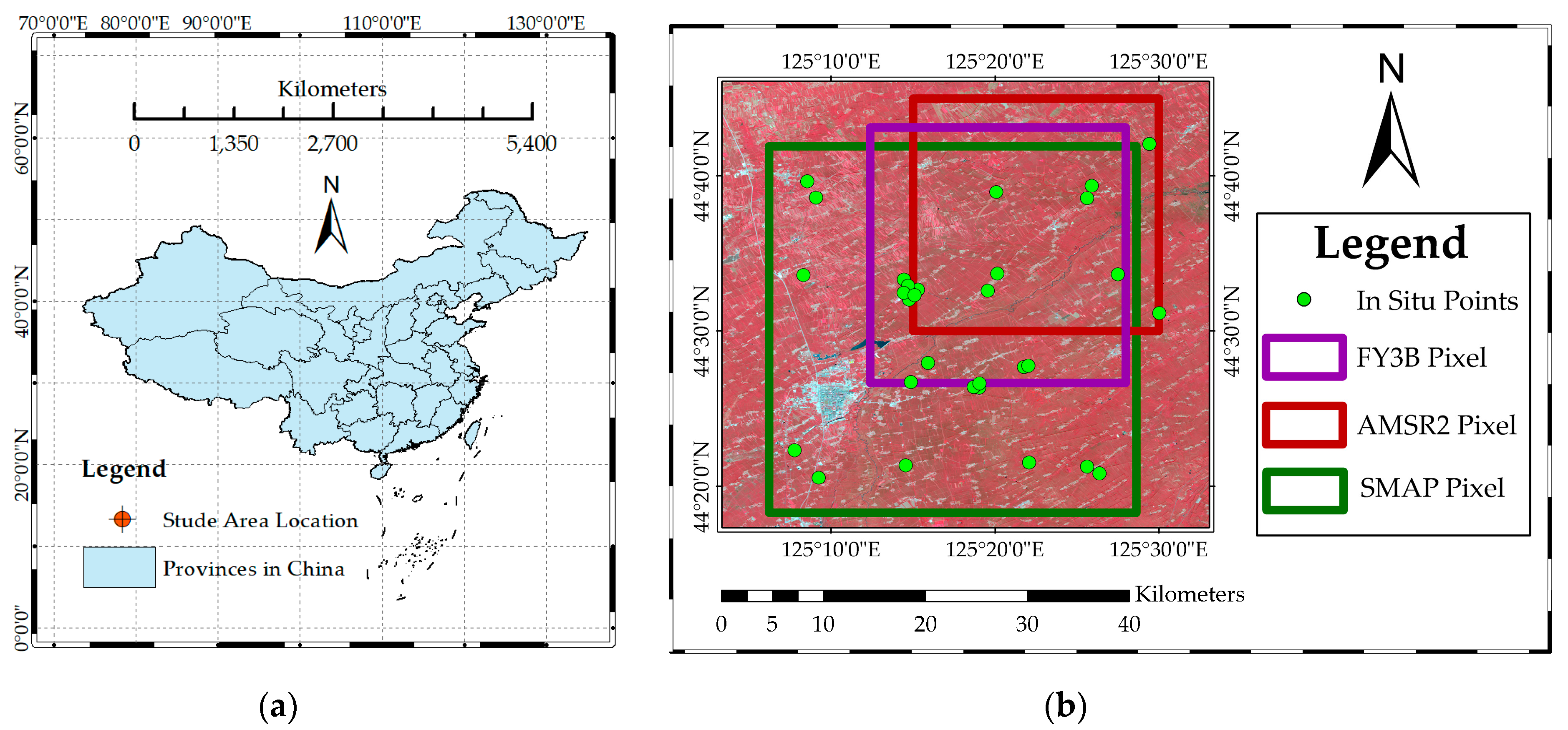
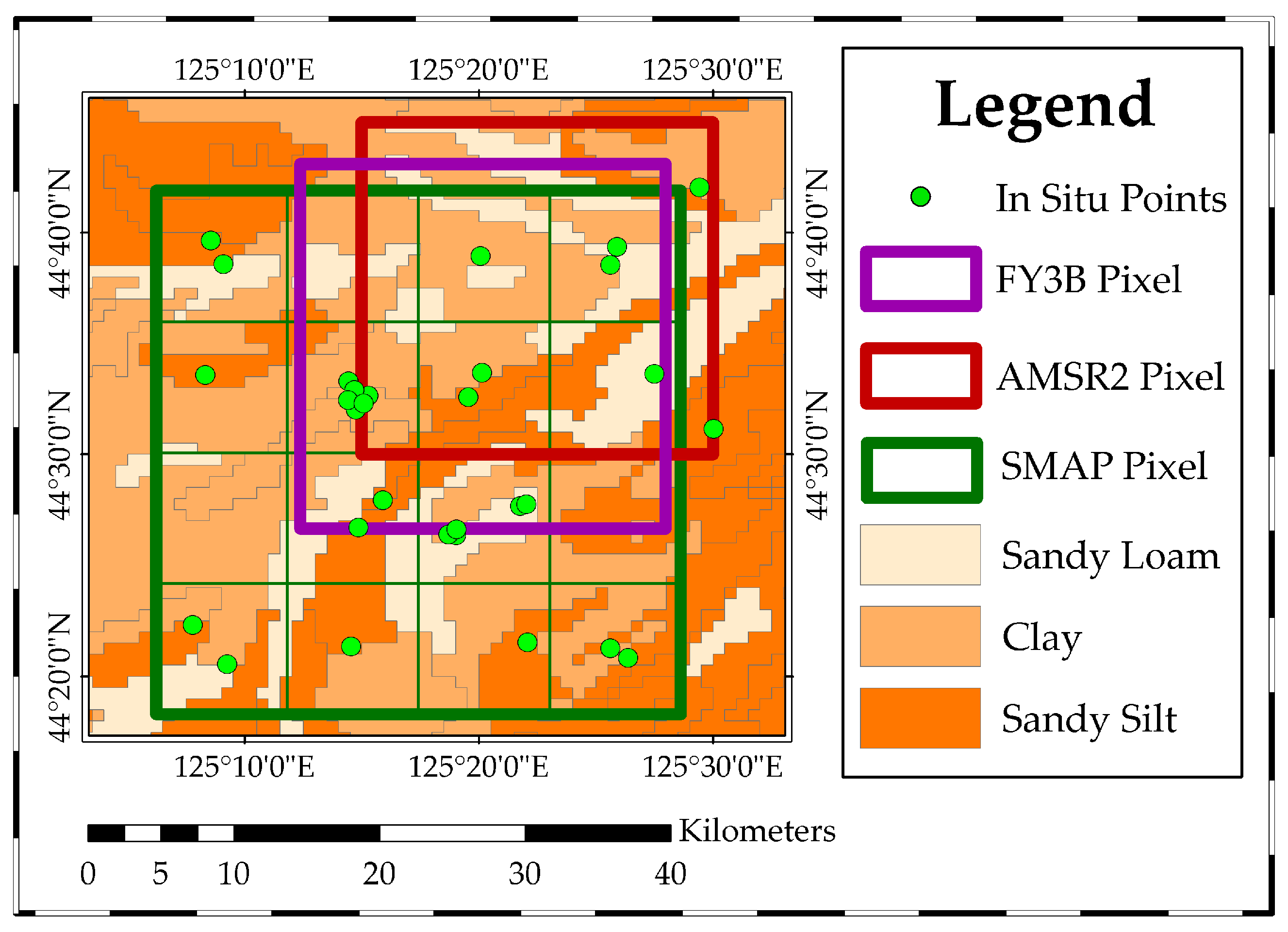
2.1. Study Area
2.2. Satellite Soil Moisture Products Based on X-Band
2.3. The In Situ Observation Network on Pixel Scale
2.3.1. Selection of Each Point Location in the In Situ Observation Network
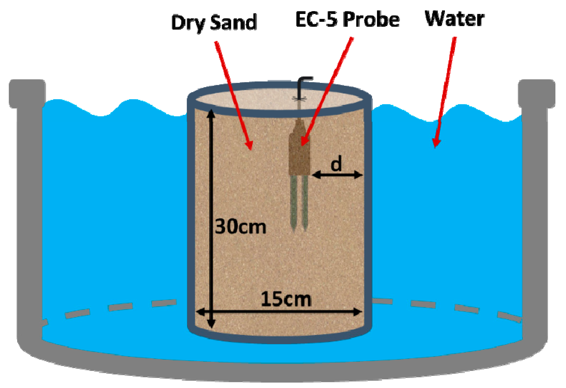
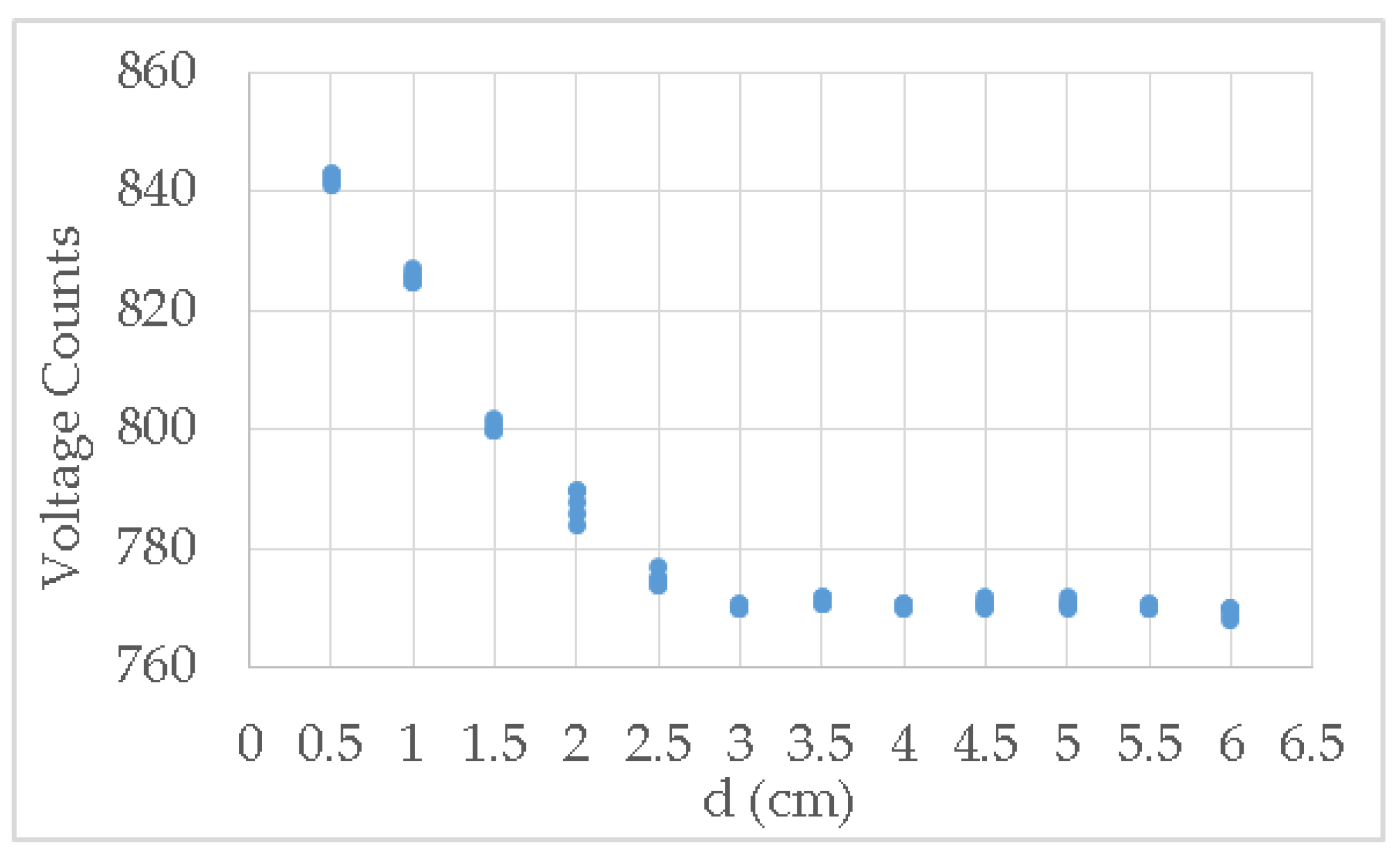
2.3.2. The Sensor Tests of the In Situ Soil Moisture
- The sensing boundary test
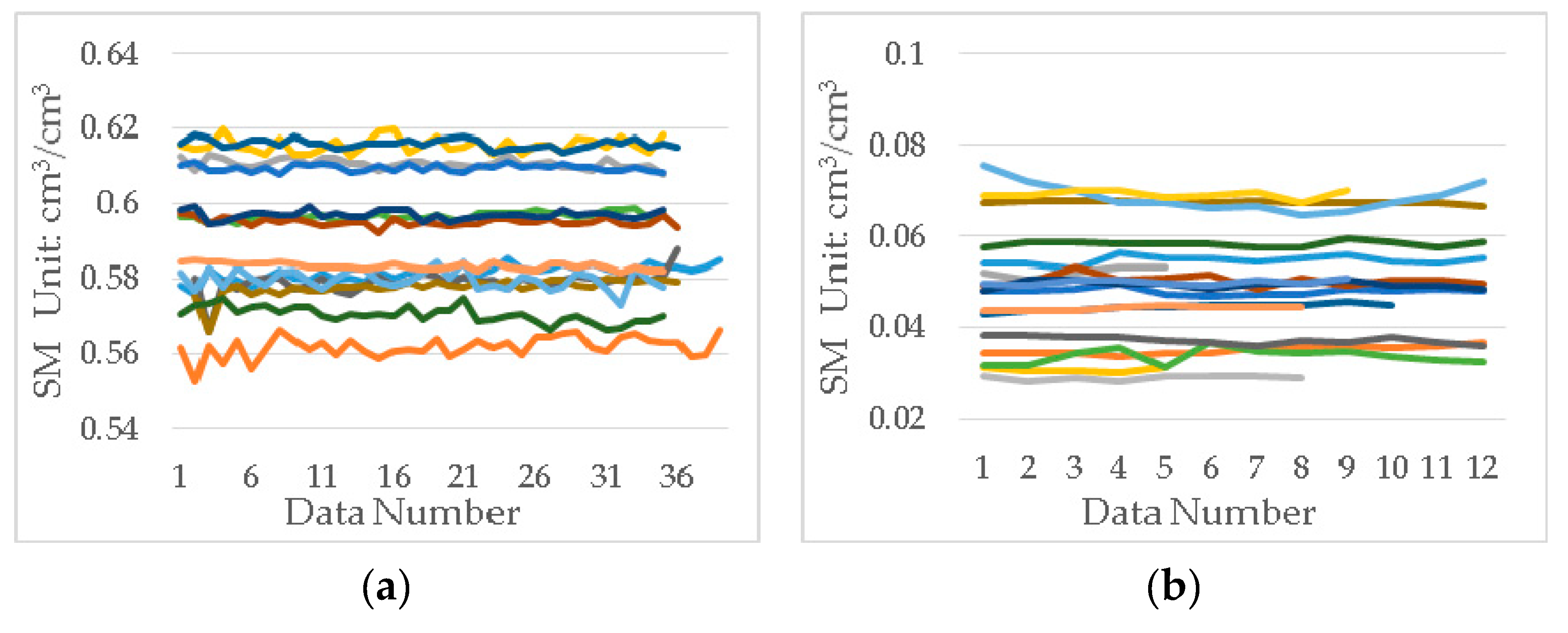
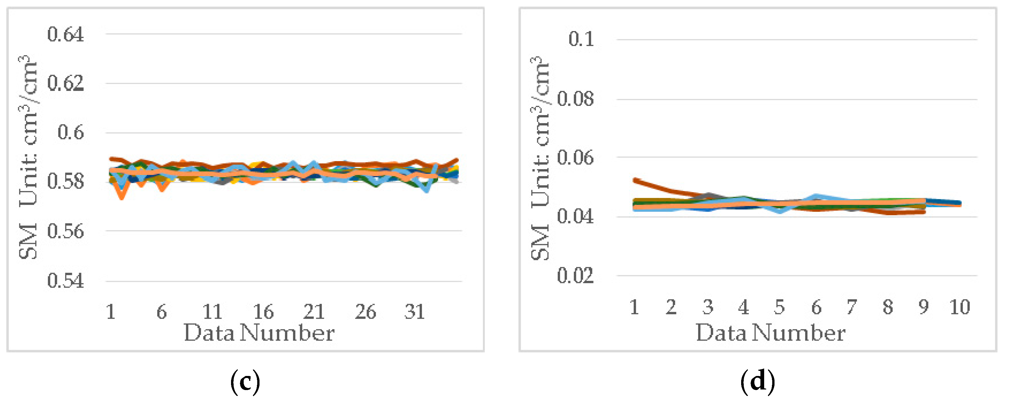
- The consistency test
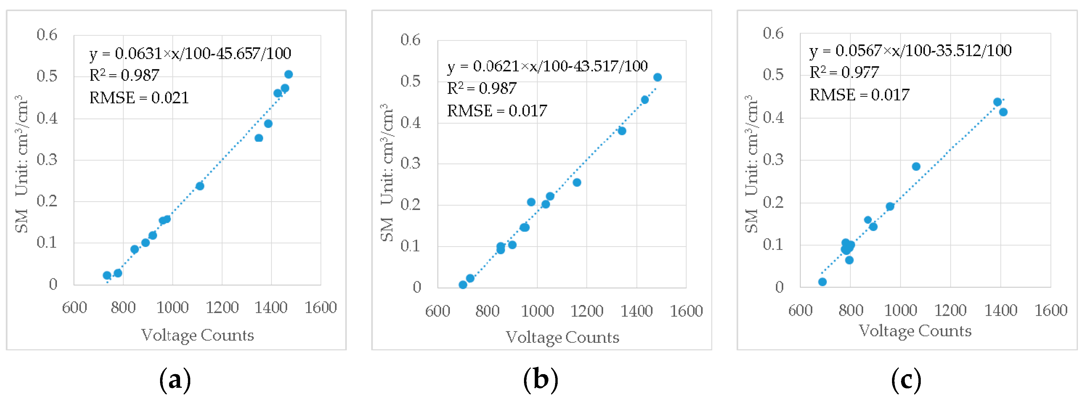
- The calibration according to actual soil from study area
2.3.3. The In Situ SST
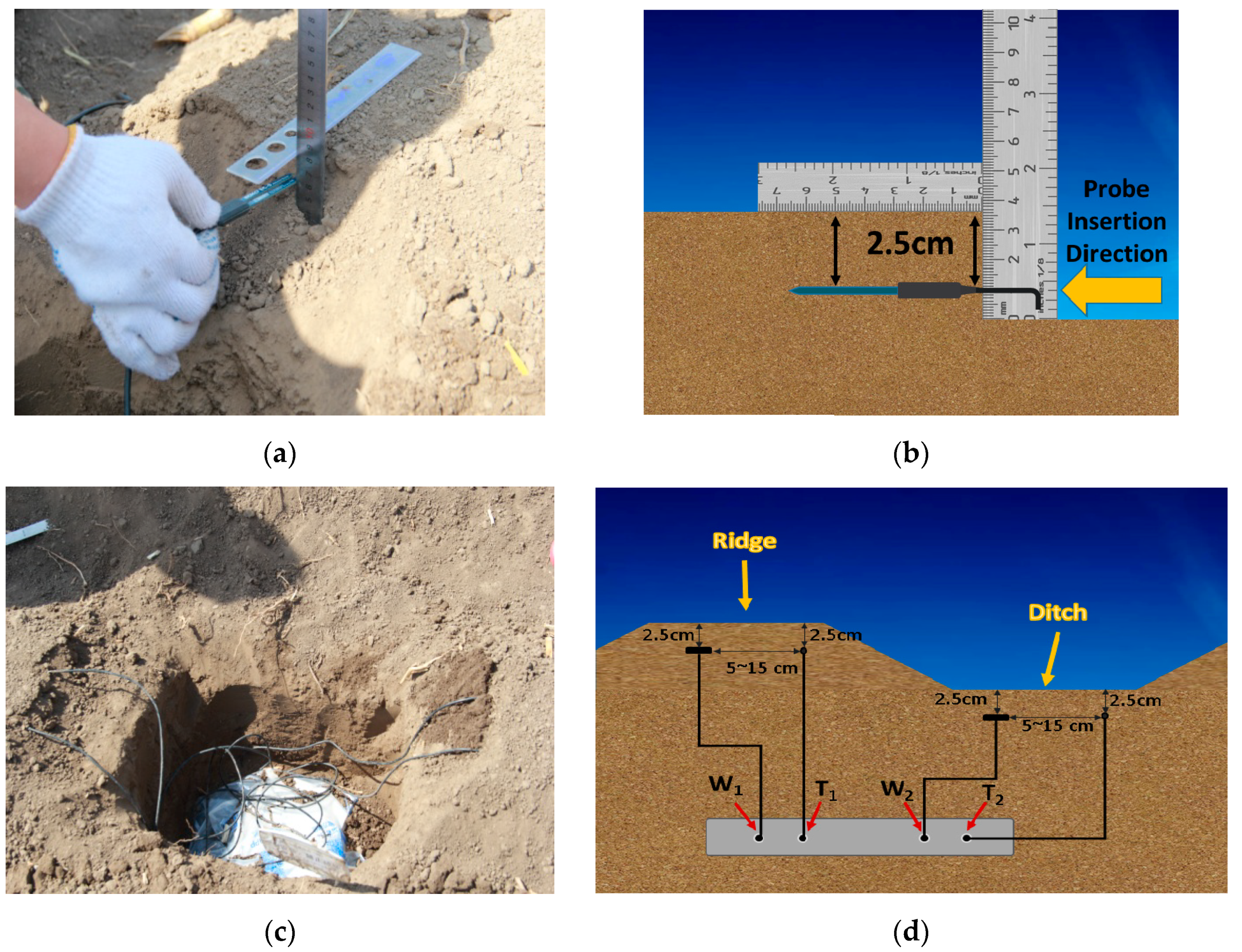
2.3.4. Placement of Sensors at In Situ Points
2.4. Ancillary Data
2.4.1. Meteorological Data
2.4.2. The Moderate Resolution Imaging Spectroradiometer (MODIS) Vegetation Index
2.4.3. The Harmonized World Soil Database
2.5. Methodology
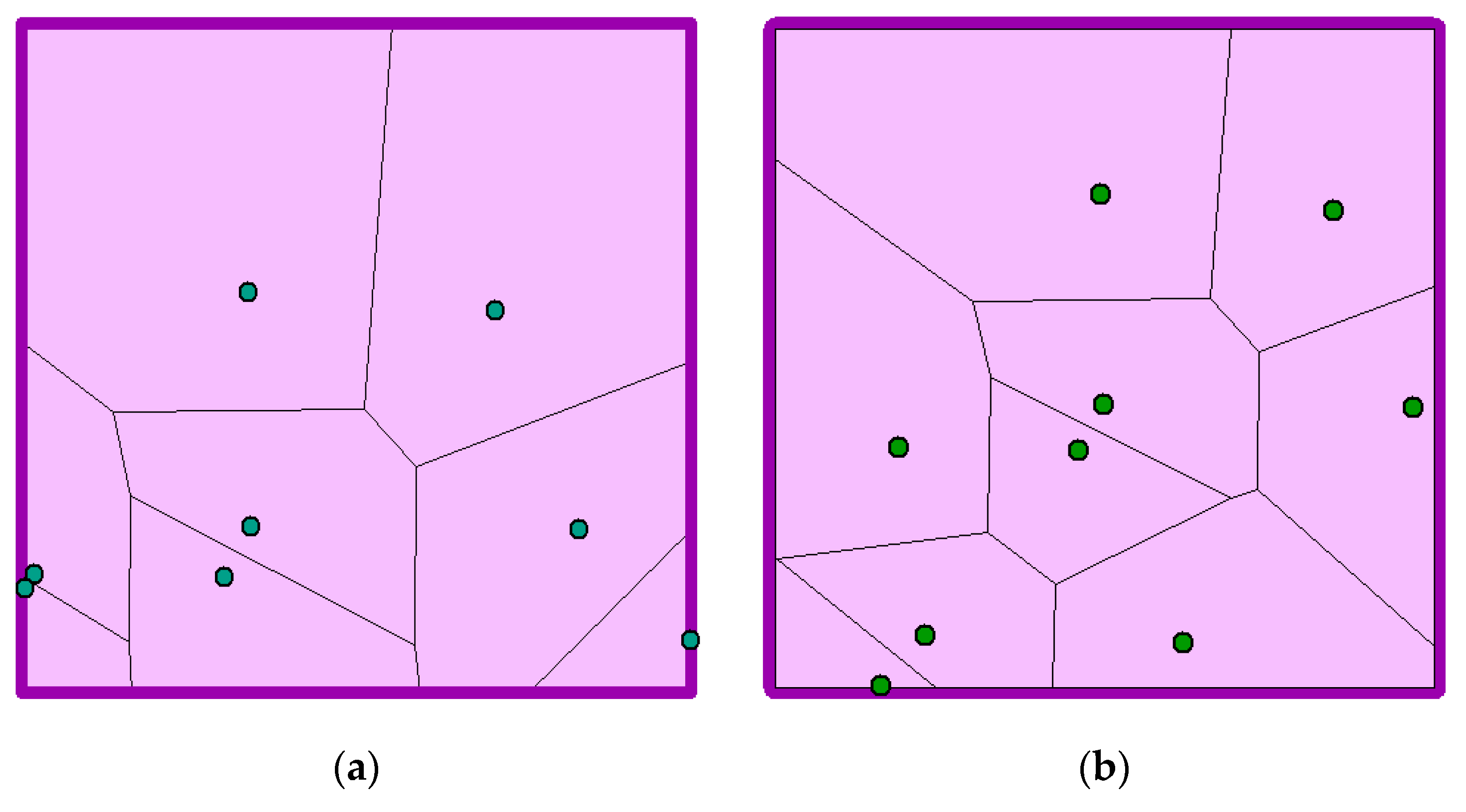
2.5.1. Thiessen Polygons Method for Pixel Scale Matching of the In Situ Data
2.5.2. The Performance Metrics for the Evaluation with In Situ Data
3. Results
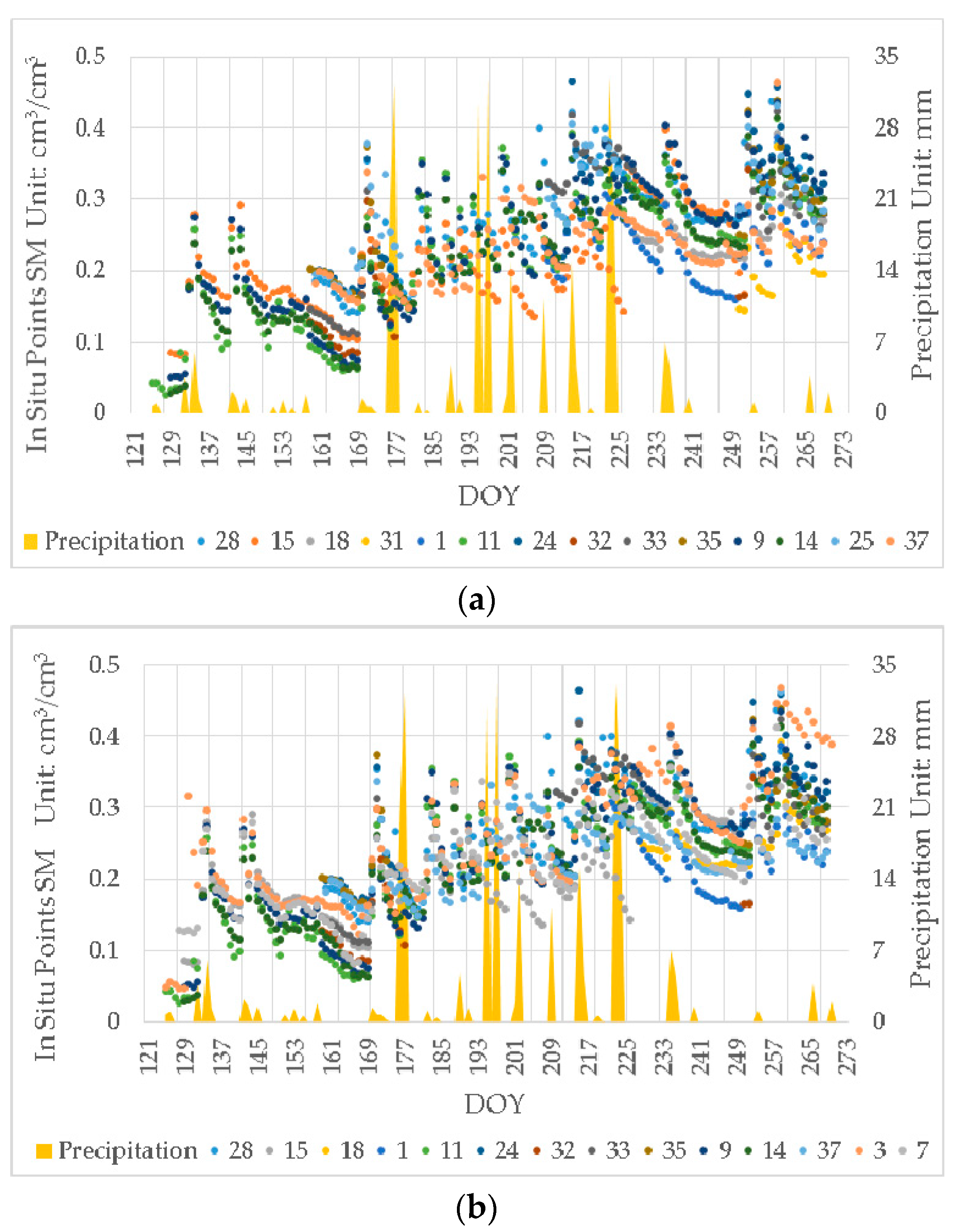
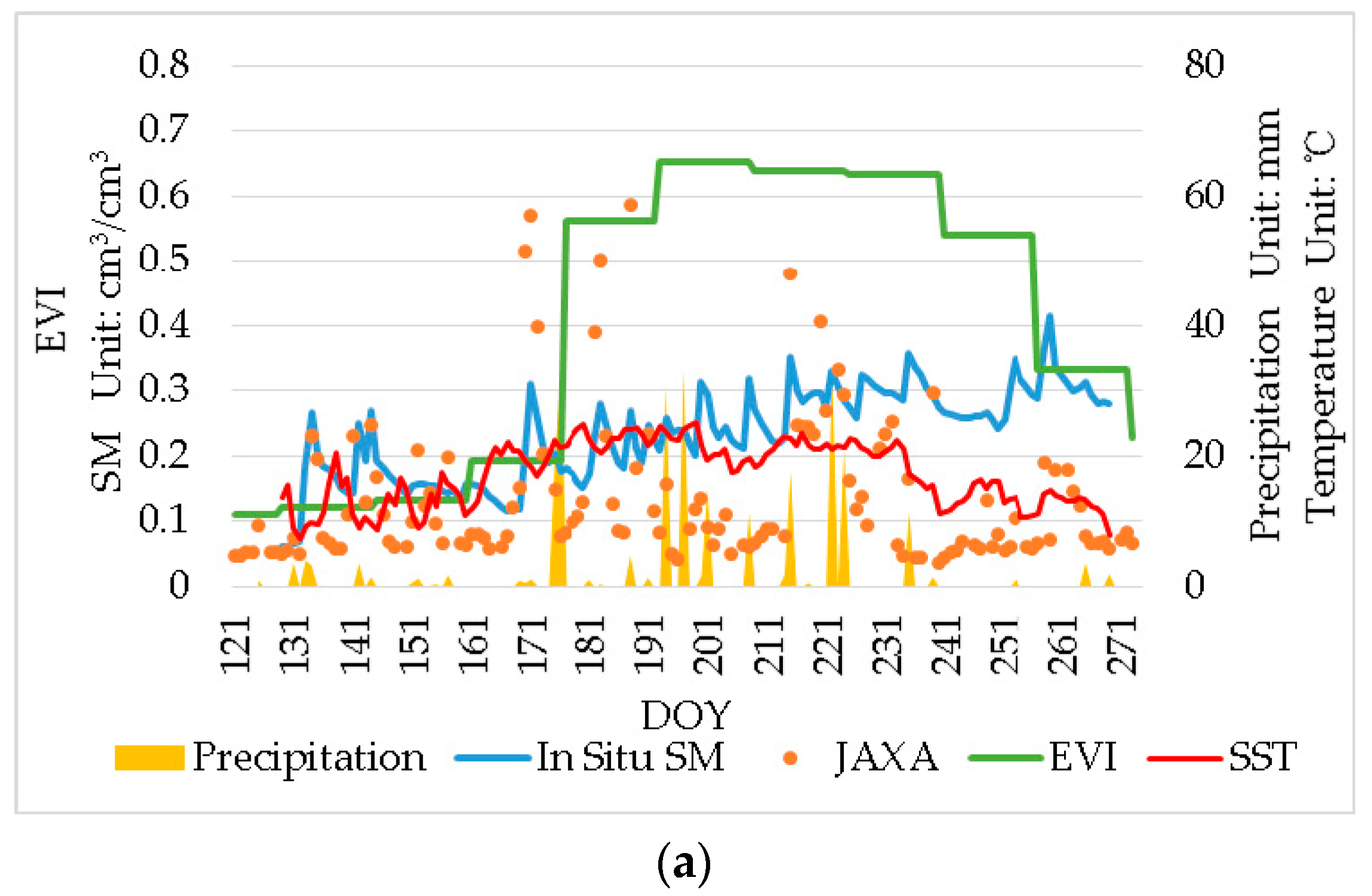
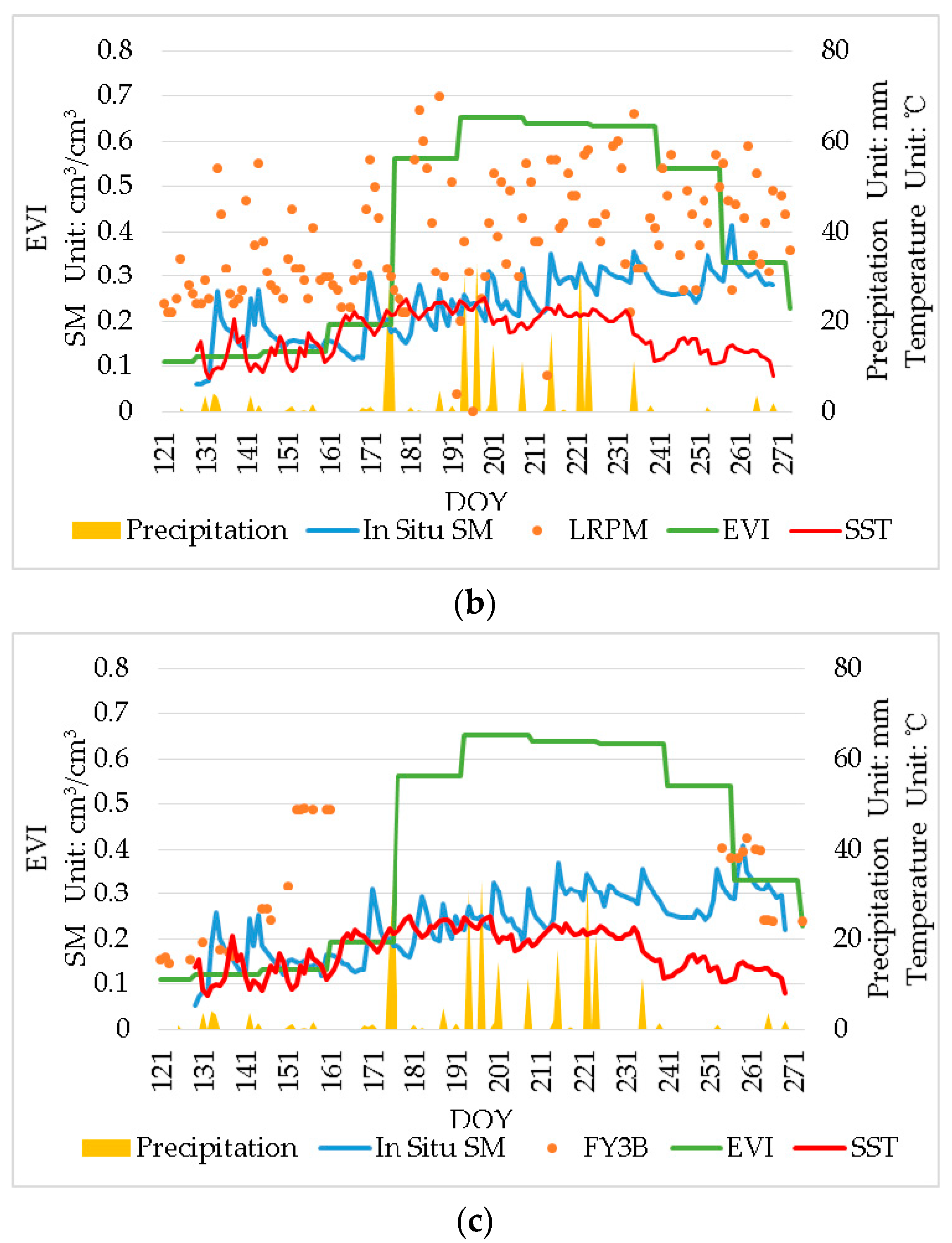
3.1. In situ Soil Moisture Data from the Network
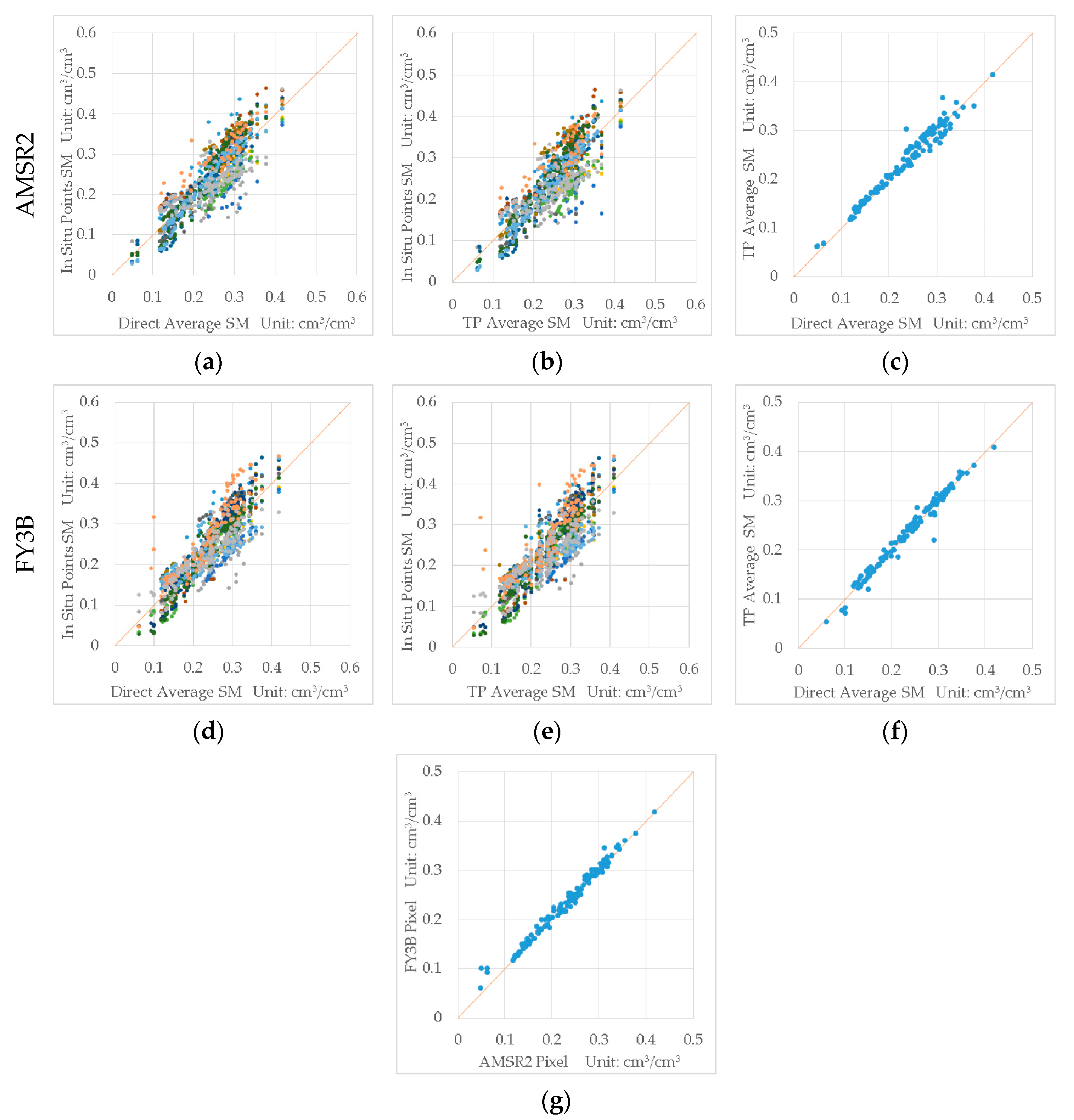
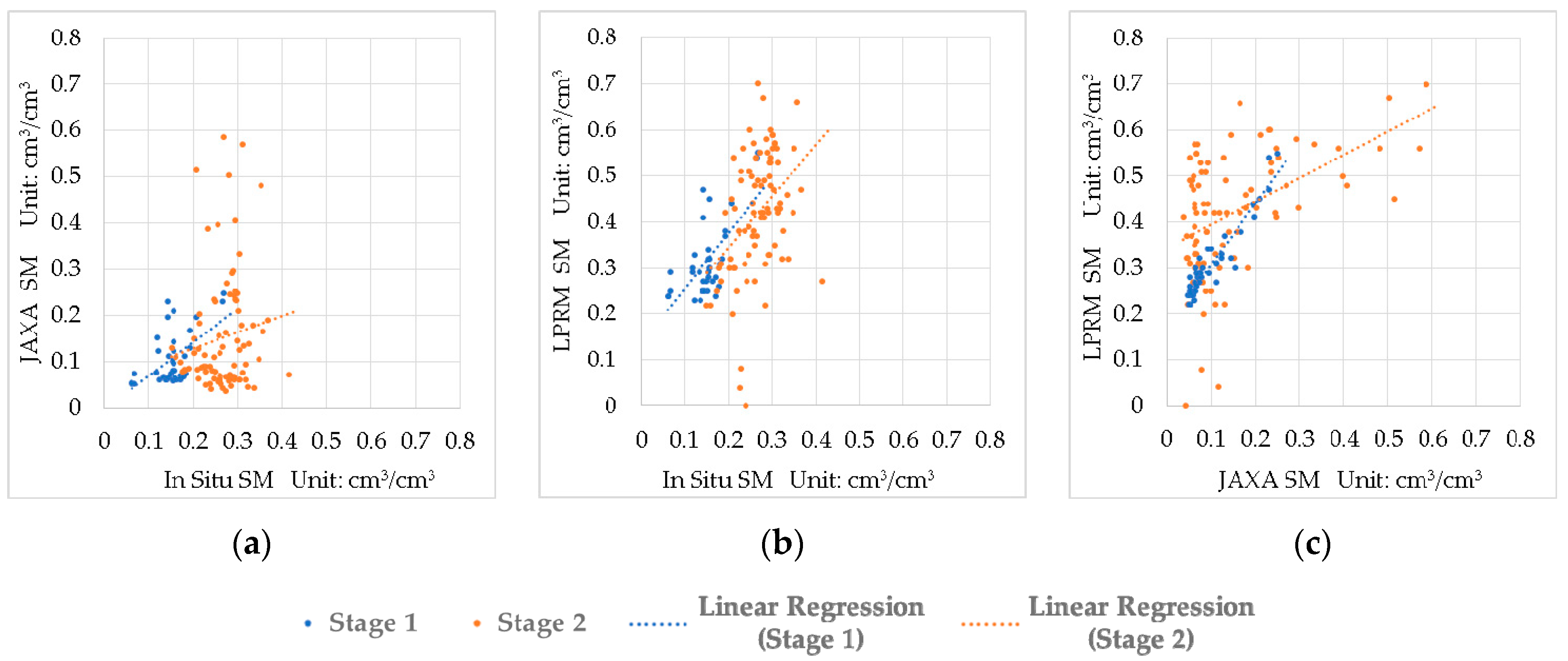
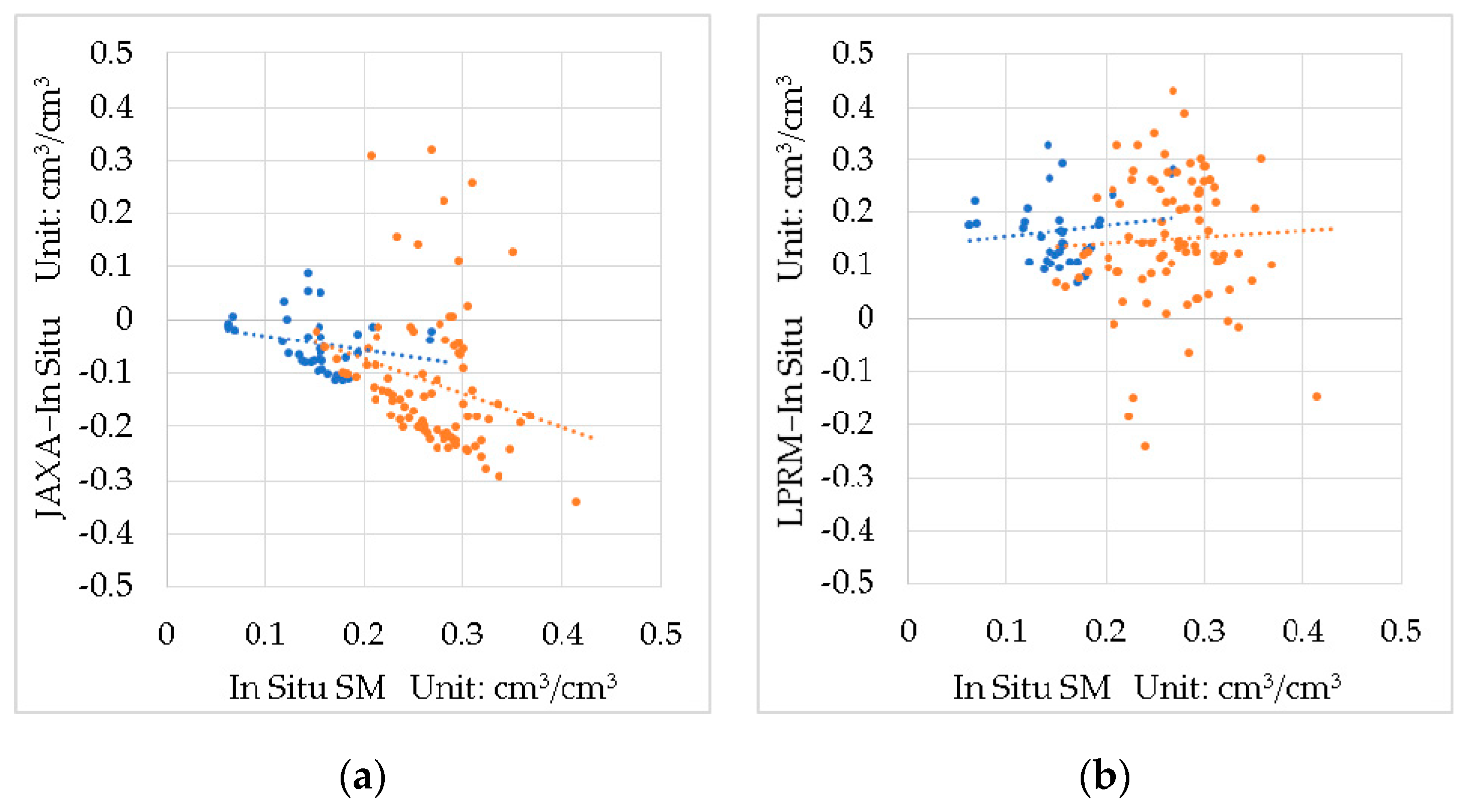
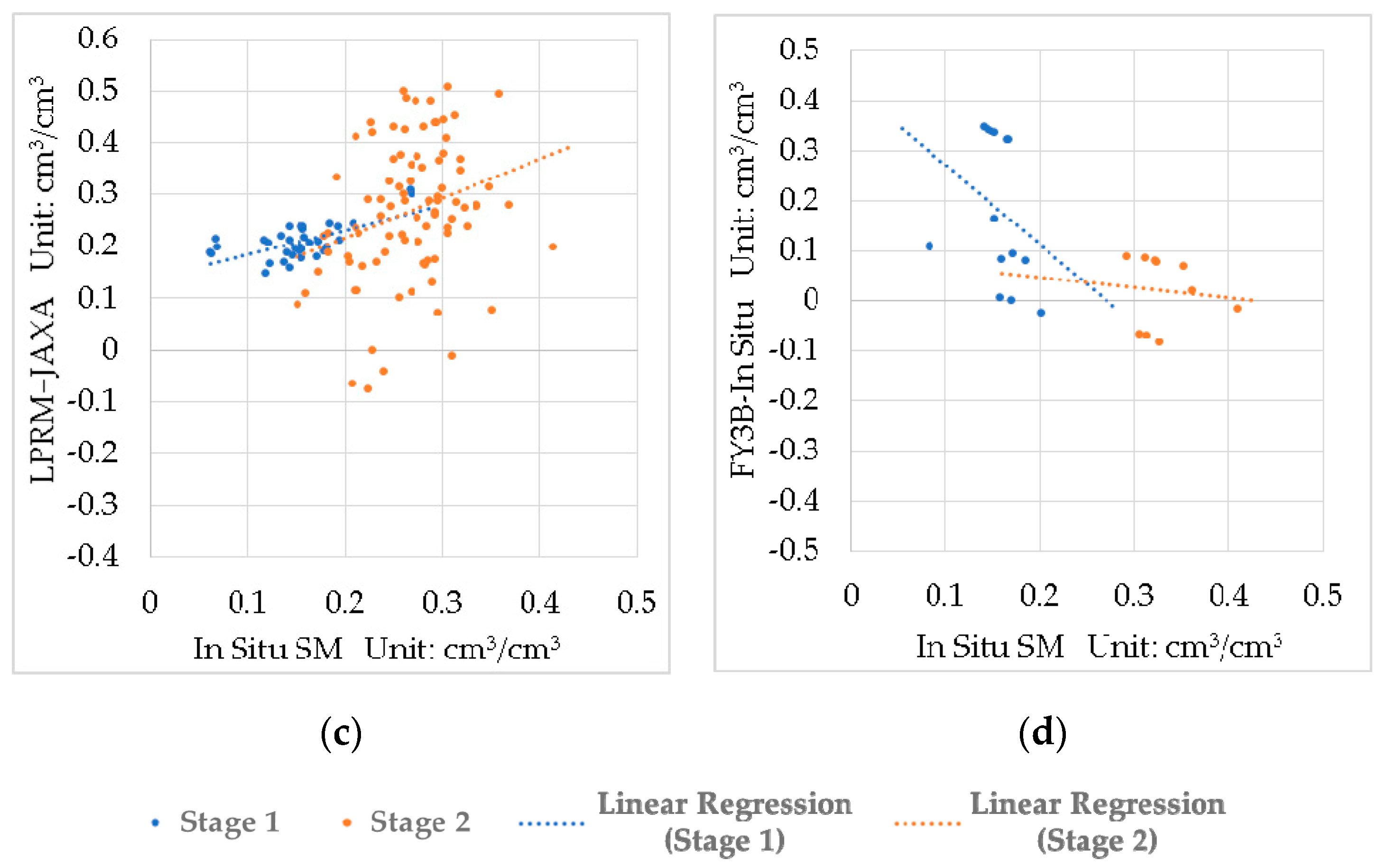
3.2. Satellite Data Evaluation and Intercomparison
4. Discussion
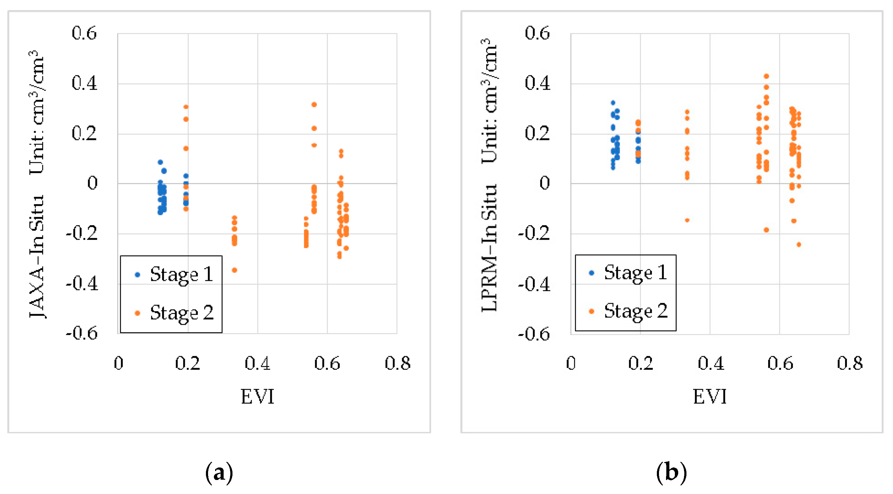
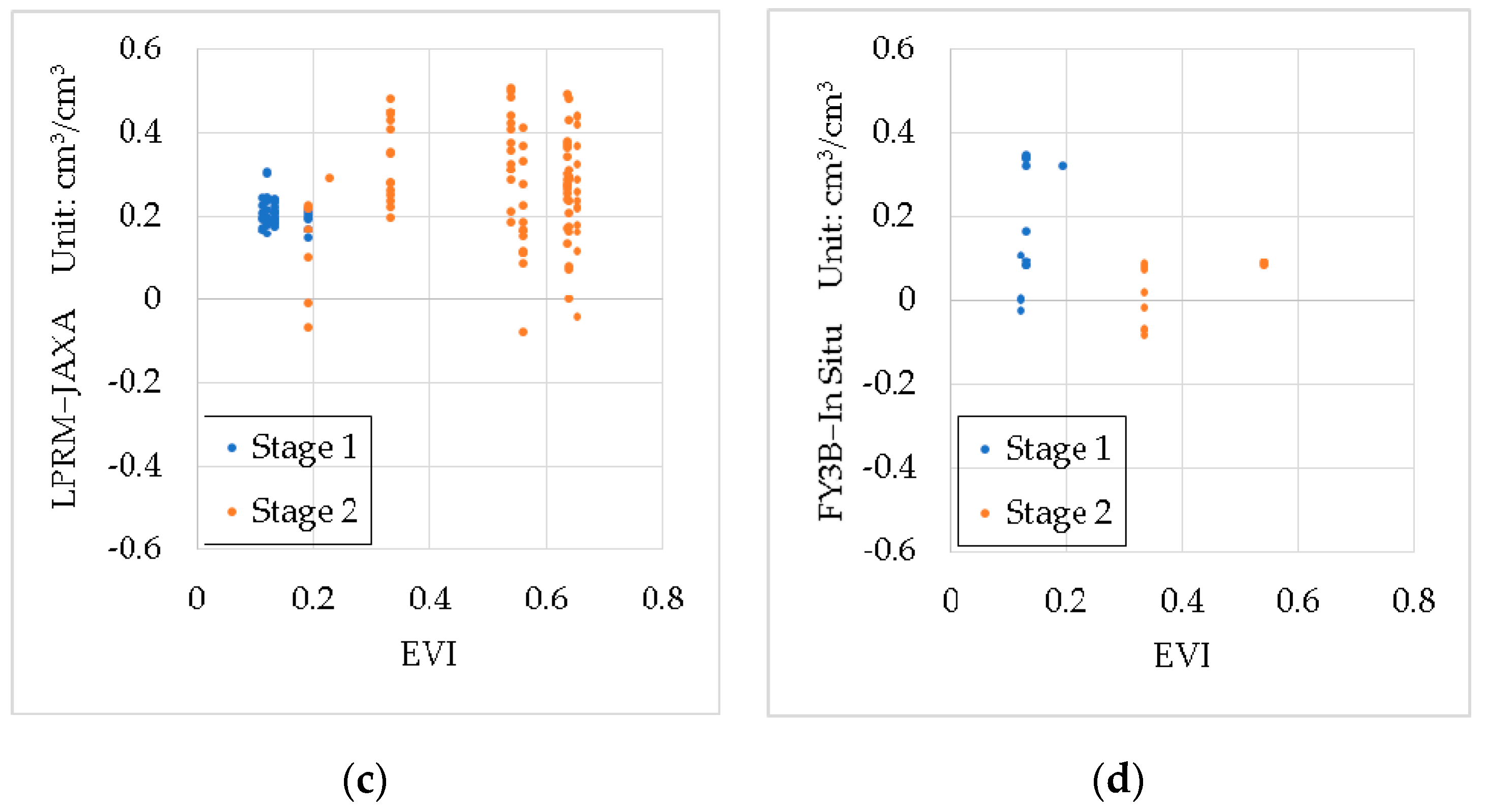
4.1. The Vegetation Cover Effect
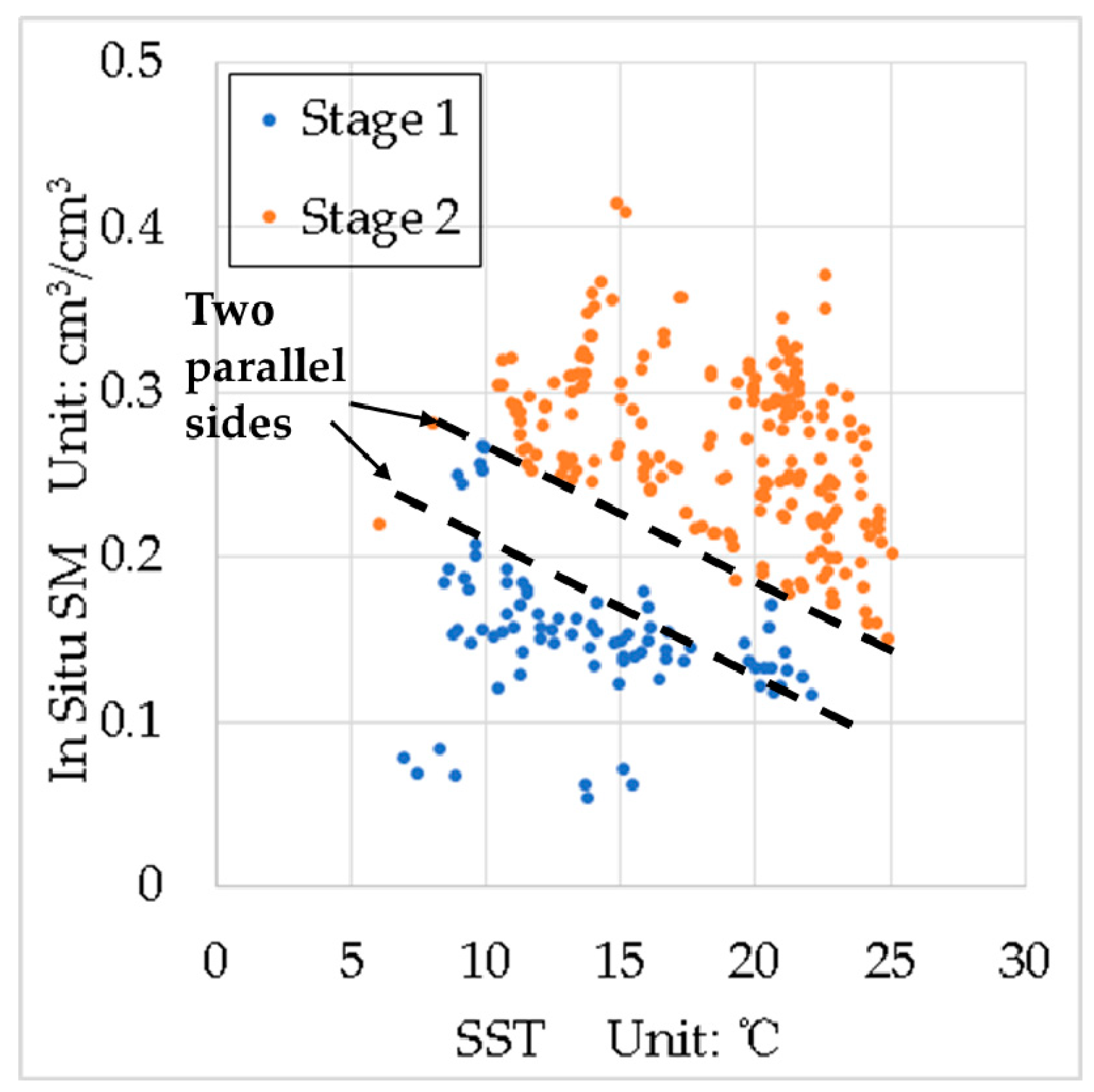
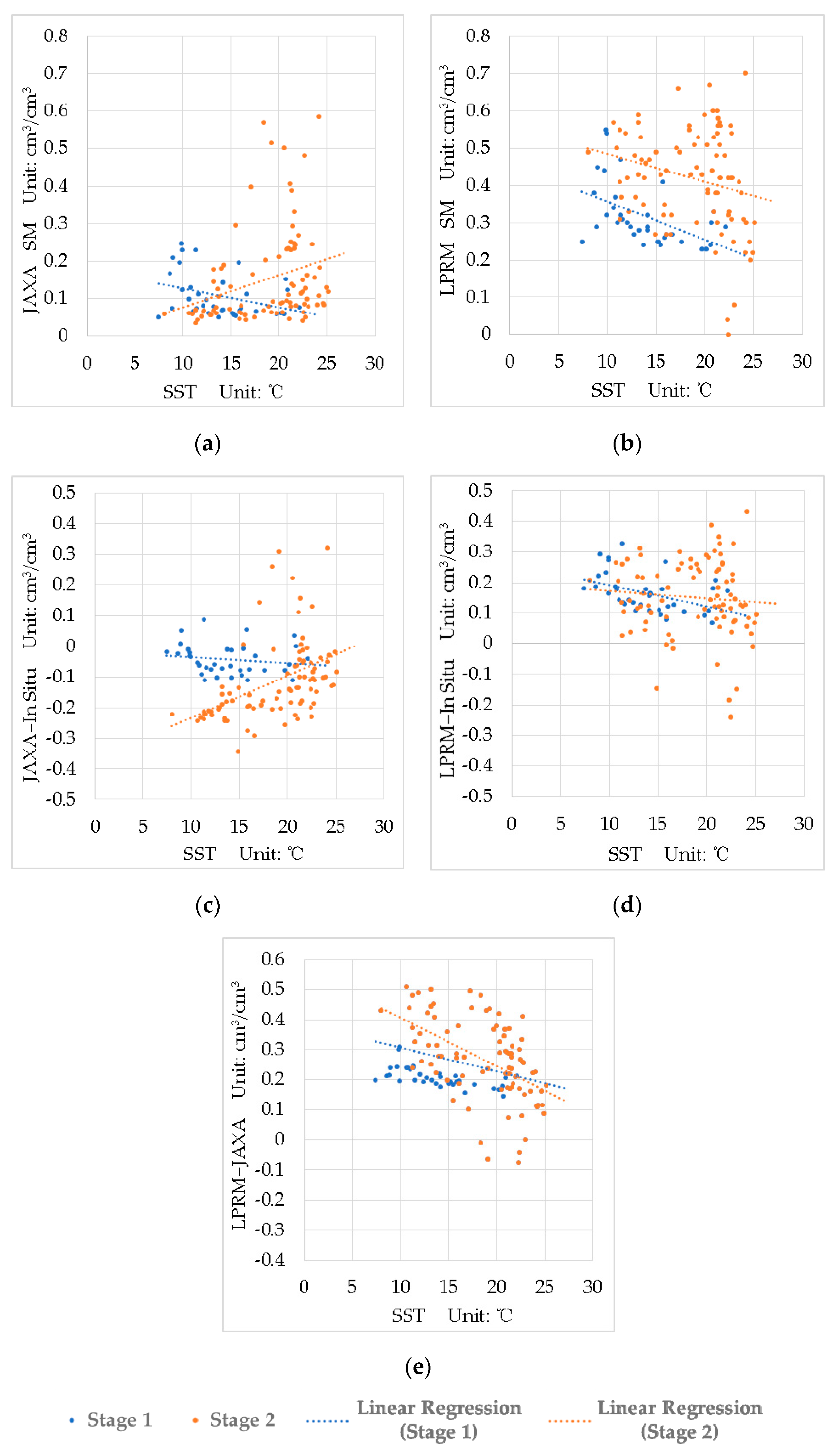
4.2. The Effect of the SST
4.3. The Actual Soil Moisture Change
5. Conclusions
Author Contributions
Funding
Acknowledgments
Conflicts of Interest
Appendix A

| Period | Products | RMSE (cm3/cm3) | ubRMSE (cm3/cm3) | b (cm3/cm3) | R |
|---|---|---|---|---|---|
| Whole Period | JAXA | 0.144 | 0.113 | −0.090 | 0.321 |
| LPRM | 0.194 | 0.109 | 0.160 | 0.551 | |
| First Stage | JAXA | 0.061 | 0.049 | −0.037 | 0.413 |
| LPRM | 0.184 | 0.063 | 0.173 | 0.579 | |
| Second Stage | JAXA | 0.167 | 0.124 | −0.112 | 0.252 |
| LPRM | 0.198 | 0.122 | 0.155 | 0.424 |
| Period | Products | RMSE (cm3/cm3) | ubRMSE (cm3/cm3) | b (cm3/cm3) | R |
|---|---|---|---|---|---|
| as FY3B | FY3B | 0.236 | 0.155 | 0.178 | 0.018 |
| JAXA | 0.228 | 0.087 | 0.211 | 0.144 | |
| LPRM | 0.232 | 0.158 | 0.170 | 0.500 |
References
- Chen, F.; Avissar, R. Impact of land-surface moisture variability on local shallow convective cumulus and precipitation in large-scale models. J. Appl. Meteorol. 1994, 33, 1382–1401. [Google Scholar] [CrossRef]
- Seneviratne, S.I.; Corti, T.; Davin, E.L.; Hirschi, M.; Jaeger, E.B.; Lehner, I.; Orlowsky, B.; Teuling, A.J.J.E.-S.R. Investigating soil moisture–climate interactions in a changing climate: A review. Earth-Sci. Rev. 2010, 99, 125–161. [Google Scholar] [CrossRef]
- Koster, R.D.; Dirmeyer, P.A.; Guo, Z.; Bonan, G.; Chan, E.; Cox, P.; Gordon, C.; Kanae, S.; Kowalczyk, E.; Lawrence, D.J.S. Regions of strong coupling between soil moisture and precipitation. Science 2004, 305, 1138–1140. [Google Scholar] [CrossRef] [PubMed]
- Gentine, P.; Polcher, J.; Entekhabi, D. Harmonic propagation of variability in surface energy balance within a coupled soil-vegetation-atmosphere system. Water Resour. Res. 2011, 47. [Google Scholar] [CrossRef]
- Seneviratne, S.I.; Lüthi, D.; Litschi, M.; Schär, C. Land–atmosphere coupling and climate change in Europe. Nature 2006, 443, 205–209. [Google Scholar] [CrossRef] [PubMed]
- Bateni, S.; Entekhabi, D. Relative efficiency of land surface energy balance components. Water Resour. Res. 2012, 48, 4. [Google Scholar] [CrossRef]
- Kędzior, M.; Zawadzki, J. SMOS data as a source of the agricultural drought information: Case study of the Vistula catchment, Poland. Geoderma 2017, 306, 167–182. [Google Scholar] [CrossRef]
- Fujii, H.; Koike, T.; Imaoka, K. Improvement of the AMSR-E algorithm for soil moisture estimation by introducing a fractional vegetation coverage dataset derived from MODIS data. J. Remote Sens. Soc. Jpn. 2009, 29, 282–292. [Google Scholar]
- Owe, M.; de Jeu, R.; Walker, J.; Zukor, D.J. A methodology for surface soil moisture and vegetation optical depth retrieval using the microwave polarization difference index. IEEE Trans. Geosci. Remote Sens. 2001, 39, 1643–1654. [Google Scholar] [CrossRef]
- Mo, T.; Choudhury, B.; Schmugge, T.; Wang, J.; Jackson, T.J. A model for microwave emission from vegetation-covered fields. J. Geophys. Res.: Oceans. 1982, 87, 11229–11237. [Google Scholar] [CrossRef]
- Jackson, T.J. Measuring surface soil moisture using passive microwave remote sensing. Hydrol. Process. 1993, 7, 139–152. [Google Scholar] [CrossRef]
- Holmes, T.R.H.; De Jeu, R.A.M.; Owe, M.; Dolman, A.J. Land surface temperature from Ka band (37 GHz) passive microwave observations. J.Geophys. Res. 2009, 114. [Google Scholar] [CrossRef]
- Kerr, Y.H.; Waldteufel, P.; Wigneron, J.-P.; Delwart, S.; Cabot, F.; Boutin, J.; Escorihuela, M.-J.; Font, J.; Reul, N.; Gruhier, C.; et al. The SMOS Mission: New Tool for Monitoring Key Elements ofthe Global Water Cycle. Proc. IEEE 2010, 98, 666–687. [Google Scholar] [CrossRef]
- Entekhabi, D.; Njoku, E.G.; O’Neill, P.E.; Kellogg, K.H.; Crow, W.T.; Edelstein, W.N.; Entin, J.K.; Goodman, S.D.; Jackson, T.J.; Johnson, J.; et al. The Soil Moisture Active Passive (SMAP) Mission. Proc. IEEE 2010, 98, 704–716. [Google Scholar] [CrossRef]
- Imaoka, K.; Maeda, T.; Kachi, M.; Kasahara, M.; Ito, N.; Nakagawa, K. Status of AMSR2 instrument on GCOM-W1. In Proceedings of Earth Observing Missions and Sensors: Development, Implementation, and Characterization II. Intern. Soc. Opt. Photonics 2012, 8528, 852815. [Google Scholar]
- Njoku, E.G.; Jackson, T.J.; Lakshmi, V.; Chan, T.K.; Nghiem, S.V. Soil moisture retrieval from AMSR-E. IEEE Trans. Geosci.Remote Sens. 2003, 41, 215–229. [Google Scholar] [CrossRef]
- Sun, R.; Zhang, Y.; Wu, S.; Yang, H.; Du, J. The FY-3B/MWRI soil moisture product and its application in drought monitoring. In Proceedings of the 2014 IEEE Geoscience and Remote Sensing Symposium, Quebec City, QC, Canada, 13–18 July 2014; pp. 3296–3298. [Google Scholar]
- Dorigo, W.; de Jeu, R.; Chung, D.; Parinussa, R.; Liu, Y.; Wagner, W.; Fernández-Prieto, D. Evaluating global trends (1988–2010) in harmonized multi-satellite surface soil moisture. Geophys. Res. Lett. 2012, 39, 18. [Google Scholar] [CrossRef]
- Cui, C.; Xu, J.; Zeng, J.; Chen, K.-S.; Bai, X.; Lu, H.; Chen, Q.; Zhao, T. Soil Moisture Mapping from Satellites: An Intercomparison of SMAP, SMOS, FY3B, AMSR2, and ESA CCI over Two Dense Network Regions at Different Spatial Scales. Remote Sens. 2017, 10, 33. [Google Scholar] [CrossRef]
- Wu, Q.; Liu, H.; Wang, L.; Deng, C. Evaluation of AMSR2 soil moisture products over the contiguous United States using in situ data from the International Soil Moisture Network. Int. J.Appl. Earth Obs.Geoinfomr. 2016, 45, 187–199. [Google Scholar] [CrossRef]
- Cho, E.; Su, C.-H.; Ryu, D.; Kim, H.; Choi, M. Does AMSR2 produce better soil moisture retrievals than AMSR-E over Australia? Remote Sens.Env. 2017, 188, 95–105. [Google Scholar] [CrossRef]
- Cho, E.; Moon, H.; Choi, M. First Assessment of the Advanced Microwave Scanning Radiometer 2 (AMSR2) Soil Moisture Contents in Northeast Asia. J. Meteorol. Soc. Japan. Ser. II 2015, 93, 117–129. [Google Scholar] [CrossRef]
- Kim, H.; Parinussa, R.; Konings, A.G.; Wagner, W.; Cosh, M.H.; Lakshmi, V.; Zohaib, M.; Choi, M. Global-scale assessment and combination of SMAP with ASCAT (active) and AMSR2 (passive) soil moisture products. Remote Sens. Env. 2018, 204, 260–275. [Google Scholar] [CrossRef]
- Bindlish, R.; Cosh, M.H.; Jackson, T.J.; Koike, T.; Fujii, H.; Chan, S.K.; Asanuma, J.; Berg, A.; Bosch, D.D.; Caldwell., T.; Collins, C.H.; McNairn, H.; Martínez-Fernández, J.; et al. GCOM-W AMSR2 soil moisture product validation using core validation sites. IEEE J. Sel. Top. Appl. Earth Obs.Remote Sens. 2018, 11, 209–219. [Google Scholar] [CrossRef]
- Kim, S.; Liu, Y.Y.; Johnson, F.M.; Parinussa, R.M.; Sharma, A. A global comparison of alternate AMSR2 soil moisture products: Why do they differ? Remote Sens. Env. 2015, 161, 43–62. [Google Scholar] [CrossRef]
- Entekhabi, D.; Reichle, R.H.; Koster, R.D.; Crow, W.T. Performance metrics for soil moisture retrievals and application requirements. J. Hydrometeorol. 2010, 11, 832–840. [Google Scholar] [CrossRef]
- Njoku, E.G.; Ashcroft, P.; Chan, T.K.; Li, L.; Sensing, R. Global survey and statistics of radio-frequency interference in AMSR-E land observations. IEEE Trans. Geosci. Remote Sens. 2005, 43, 938–947. [Google Scholar] [CrossRef]
- Li, L.; Njoku, E.G.; Im, E.; Chang, P.S.; Germain, K.; Sensing, R. A preliminary survey of radio-frequency interference over the US in Aqua AMSR-E data. IEEE Trans. Geosci. Remote Sens.. 2004, 42, 380–390. [Google Scholar] [CrossRef]
- Njoku, E.; Chan, S. Vegetation and surface roughness effects on AMSR-E land observations. Remote Sens. Env. 2006, 100, 190–199. [Google Scholar] [CrossRef]
- Jackson, T.J.; Schmugge, T.J. Vegetation Effects on Microwave Emission of soils. Remote Sens. Env. 1991, 36, 203–212. [Google Scholar] [CrossRef]
- Draper, C.S.; Walker, J.P.; Steinle, P.J.; De Jeu, R.A.; Holmes, T.R.H. An evaluation of AMSR–E derived soil moisture over Australia. Remote Sens. Env. 2009, 113, 703–710. [Google Scholar] [CrossRef]
- de Jeu, R.A.M.; Wagner, W.; Holmes, T.R.H.; Dolman, A.J.; van de Giesen, N.C.; Friesen, J. Global Soil Moisture Patterns Observed by Space Borne Microwave Radiometers and Scatterometers. Surv. Geophys. 2008, 29, 399–420. [Google Scholar] [CrossRef]
- Maeda, T.; Taniguchi, Y. Descriptions of GCOM-W1 AMSR2 Level 1R and Level 2 Algorithms. Available online: https://suzaku.eorc.jaxa.jp/GCOM_W/data/doc/NDX-120015A.pdf (accessed on 21 February 2019).
- Lu, H.; Koike, T.; Fujii, H.; Ohta, T.; Tamagawa, K. Development of a physically-based soil moisture retrieval algorithm for spaceborne passive microwave radiometers and its application to AMSR-E. J. Remote Sens. Soc. Jpn. 2009, 29, 253–262. [Google Scholar]
- Owe, M.; de Jeu, R.; Holmes, T. Multisensor historical climatology of satellite-derived global land surface moisture. J. Geophys. Res. Earth Surf. 2008, 113, F1. [Google Scholar] [CrossRef]
- Meesters, A.G.; De Jeu, R.A.; Owe, M.; Letters, R.S. Analytical derivation of the vegetation optical depth from the microwave polarization difference index. IEEE Geosci. Remote Sens. Lett.. 2005, 2, 121–123. [Google Scholar] [CrossRef]
- Shi, J.; Jiang, L.; Zhang, L.; Chen, K.-S.; Wigneron, J.-P.; Chanzy, A.; Jackson, J.P.; Sensing, R. Physically based estimation of bare-surface soil moisture with the passive radiometers. IEEE Trans.Geosci. Remote Sens. 2006, 44, 3145–3153. [Google Scholar] [CrossRef]
- Jackson, T.J.; Le Vine, D.M.; Hsu, A.Y.; Oldak, A.; Starks, P.J.; Swift, C.T.; Isham, J.D.; Haken, M. Soil moisture mapping at regional scales using microwave radiometry: The Southern Great Plains Hydrology Experiment. IEEE Trans. Geosci. Remote Sens. 1999, 37, 2136–2151. [Google Scholar] [CrossRef]
- MODIS vegetation index user’s guide (MOD13 Series). Available online: https://icdc.cen.uni-hamburg.de/fileadmin/user_upload/icdc_Dokumente/MODIS/MODIS_Collection6_VegetationIndex_UsersGuide_MOD13_V03_June2015.pdf (accessed on 21 February 2019).
- Şen, Z. Average areal precipitation by percentage weighted polygon method. J. Hydrologic Engineering. 1998, 3, 69–72. [Google Scholar] [CrossRef]
- Rhynsburger, D. Analytic delineation of Thiessen polygons. Geogr. Anal. 1973, 5, 133–144. [Google Scholar] [CrossRef]
- Song, C.; Jia, L. A Method for Downscaling FengYun-3B Soil Moisture Based on Apparent Thermal Inertia. Remote Sens. 2016, 8, 703. [Google Scholar] [CrossRef]
- Wang, G.; Hagan, D.F.T.; Lou, D.; Chen, T. Evaluation of soil moisture derived from FY3B microwave brightness temperature over the Tibetan Plateau. Remote Sens. Lett. 2016, 7, 817–826. [Google Scholar] [CrossRef]
- Brocca, L.; Hasenauer, S.; Lacava, T.; Melone, F.; Moramarco, T.; Wagner, W.; Dorigo, W.; Matgen, P.; Martínez-Fernández, J.; Llorens, P.; et al. Soil moisture estimation through ASCAT and AMSR-E sensors: An intercomparison and validation study across Europe. Remote Sens. Env. 2011, 115, 3390–3408. [Google Scholar] [CrossRef]
- Parinussa, R.M.; Holmes, T.R.H.; De Jeu, R.A.M. Soil Moisture Retrievals From the WindSat Spaceborne Polarimetric Microwave Radiometer. IEEE Trans. Geosci. Remote Sens. 2012, 50, 2683–2694. [Google Scholar] [CrossRef]
- Parinussa, R.M.; Wang, G.; Holmes, T.R.H.; Liu, Y.Y.; Dolman, A.J.; De Jeu, R.A.M.; Jiang, T.; Zhang, P.; Shi, J. Global surface soil moisture from the Microwave Radiation Imager onboard the Fengyun-3B satellite. Int. J Remote Sens. 2014, 35, 7007–7029. [Google Scholar] [CrossRef]


| Soil Texture | Clay (%) | Silt (%) | Sand (%) |
|---|---|---|---|
| Sandy Loam Soil | 12.41 | 64.28 | 23.31 |
| Clay Soil | 11.80 | 57.71 | 30.48 |
| Sandy Silt Soil | 11.81 | 55.87 | 32.32 |
| Sensing Range (cm) | 2.5~3 |
| Operating Temperature (°C) | −40~+60 |
| Measurement Range of SM (%) | 0~100 |
| Accuracy (cm3/cm3) | 0.02 |
| Period | Products | RMSE (cm3/cm3) | ubRMSE (cm3/cm3) | b (cm3/cm3) | R |
|---|---|---|---|---|---|
| Whole Period | JAXA | 0.150 | 0.117 | −0.094 | 0.259 |
| LPRM | 0.191 | 0.110 | 0.156 | 0.542 | |
| First Stage | JAXA | 0.066 | 0.049 | −0.043 | 0.565 |
| LPRM | 0.177 | 0.063 | 0.166 | 0.654 | |
| Second Stage | JAXA | 0.173 | 0.129 | −0.115 | 0.136 |
| LPRM | 0.196 | 0.124 | 0.152 | 0.403 |
| Period | Products | RMSE (cm3/cm3) | ubRMSE (cm3/cm3) | b (cm3/cm3) | R |
|---|---|---|---|---|---|
| as FY3B | FY3B | 0.237 | 0.155 | 0.179 | 0.042 |
| JAXA | 0.231 | 0.085 | 0.215 | 0.180 | |
| LPRM | 0.233 | 0.156 | 0.174 | 0.516 |
© 2019 by the authors. Licensee MDPI, Basel, Switzerland. This article is an open access article distributed under the terms and conditions of the Creative Commons Attribution (CC BY) license (http://creativecommons.org/licenses/by/4.0/).
Share and Cite
Fu, H.; Zhou, T.; Sun, C. Evaluation and Analysis of AMSR2 and FY3B Soil Moisture Products by an In Situ Network in Cropland on Pixel Scale in the Northeast of China. Remote Sens. 2019, 11, 868. https://doi.org/10.3390/rs11070868
Fu H, Zhou T, Sun C. Evaluation and Analysis of AMSR2 and FY3B Soil Moisture Products by an In Situ Network in Cropland on Pixel Scale in the Northeast of China. Remote Sensing. 2019; 11(7):868. https://doi.org/10.3390/rs11070868
Chicago/Turabian StyleFu, Haoyang, Tingting Zhou, and Chenglin Sun. 2019. "Evaluation and Analysis of AMSR2 and FY3B Soil Moisture Products by an In Situ Network in Cropland on Pixel Scale in the Northeast of China" Remote Sensing 11, no. 7: 868. https://doi.org/10.3390/rs11070868
APA StyleFu, H., Zhou, T., & Sun, C. (2019). Evaluation and Analysis of AMSR2 and FY3B Soil Moisture Products by an In Situ Network in Cropland on Pixel Scale in the Northeast of China. Remote Sensing, 11(7), 868. https://doi.org/10.3390/rs11070868