Article

Analysis of Four Years of Global XCO2 Anomalies as Seen by Orbiting Carbon Observatory-2

1
Finnish Meteorological Institute, 00560 Helsinki, Finland
2
Center for Global Environmental Research, National Institute for Environmental Studies, Tsukuba 305-0053, Japan
3
Jet Propulsion Laboratory/California Institute of Technology, Pasadena, CA 91109, USA
*
Author to whom correspondence should be addressed.
Remote Sens. 2019, 11(7), 850; https://doi.org/10.3390/rs11070850
Submission received: 27 February 2019 / Revised: 2 April 2019 / Accepted: 4 April 2019 / Published: 9 April 2019
(This article belongs to the Special Issue Remote Sensing of Carbon Dioxide and Methane in Earth’s Atmosphere)

Abstract

:
NASA’s carbon dioxide mission, Orbiting Carbon Observatory-2, began operating in September 2014. In this paper, we analyze four years (2015–2018) of global (60°S–60°N) XCO2 anomalies and their annual variations and seasonal patterns. We show that the anomaly patterns in the column-averaged CO2 dry air mole fraction, XCO2, are robust and consistent from year-to-year. We evaluate the method by comparing the anomalies to fluxes from anthropogenic, biospheric, and biomass burning and to model-simulated local concentration enhancements. We find that, despite the simplicity of the method, the anomalies describe the spatio-temporal variability of XCO2 (including anthropogenic emissions and seasonal variability related to vegetation and biomass burning) consistently with more complex model-based approaches. We see, for example, that positive anomalies correspond to fossil fuel combustion over the major industrial areas (e.g., China, eastern USA, central Europe, India, and the Highveld region in South Africa), shown as large positive XCO2 enhancements in the model simulations. We also find corresponding positive anomalies and fluxes over biomass burning areas during different fire seasons. On the other hand, the largest negative anomalies correspond to the growing season in the northern middle latitudes, characterized by negative XCO2 enhancements from simulations and high solar-induced chlorophyll fluorescence (SIF) values (indicating the occurrence of photosynthesis). The largest discrepancies between the anomaly patterns and the model-based results are observed in the tropical regions, where OCO-2 shows persistent positive anomalies over every season of every year included in this study. Finally, we demonstrate how XCO2 anomalies enable the detection of anthropogenic signatures for several local scale case studies, both in the Northern and Southern Hemisphere. In particular, we analyze the XCO2 anomalies collocated with the recent TROPOspheric Monitoring Instrument NO2 observations (used as indicator of anthropogenic fossil fuel combustion) over the Highveld region in South Africa. The results highlight the capability of satellite-based observations to monitor natural and man-made CO2 signatures on global scale.

1. Introduction

The first routine measurements of atmospheric carbon dioxide (CO2) were started at Mauna Loa Observatory in 1958 by Charles David Keeling. These measurements now form the iconic Keeling curve that shows, in addition to seasonal variations, rapidly increasing levels of CO2 in the atmosphere due to the burning of fossil fuels. Now, 60 years later, atmospheric CO2 concentrations are measured all over the world and show levels that are about 100 ppm higher than they were in 1958, when they were about 315 ppm. However, the measurement networks are still denser in the Western world.
One of the most important applications of CO2 measurements is to infer the surface CO2 fluxes, i.e., sources and sinks (or emissions into and removal from the atmosphere). A variety of methods are commonly used to derive CO2 fluxes from spatially resolved estimates of column-averaged CO2 dry air mole fraction, XCO2. These methods can be broadly classified as analytic mass balance, plume dispersion, or atmospheric inversion methods. All three approaches predict or optimize surface fluxes needed to reproduce the observed XCO2 distribution in the presence of the time-varying wind field. Ground-based in situ measurements provide the best available constraints on CO2 concentrations, but the existing ground based network is unevenly distributed and includes few stations in the tropics, high latitudes, or over the ocean. One way to extend this network is to use space-based measurements of the XCO2 [1,2]. The main advantage of space-based observations is that they can provide high spatial and temporal resolution on global scale with the same measurement device. The principal challenge is the need for unprecedented levels of precision and accuracy to resolve and quantify CO2 fluxes. High precision measurements are needed to clearly resolve CO2 concentration anomalies in the context of their large background concentrations. For example, source pixel mass balance methods [3] indicate that a single-sounding precision of ~ 0.25 % (~1 part per million (ppm) out of the 400 ppm background) is needed within a 4 square km satellite footprint to detect a ~10 kiloton/day CO2 source in the presence of a ~5 km/h wind. Spatially and temporally coherent biases in the measurements must also be minimized because, regional-scale biases in XCO2 no larger than a few tenths of a part per million can introduce carbon flux errors exceeding 0.7 Gigatons of carbon per year [4,5]. Ideally, the inverse modeling systems that estimate CO2 fluxes from atmospheric measurements, can assimilate information from all available measurement types.
The first space-based instrument designed to retrieve estimates of XCO2 throughout the atmospheric column from high resolution spectra of reflected sunlight was SCIAMACHY (Scanning Imaging Absorption Spectrometer for Atmospheric Chartography), launched by the European Space Agency onboard the Envisat spacecraft in 2002 [6]. The first mission that provided XCO2 measurements at a precision better than 0.6% is the Japanese GOSAT (Greenhouse Gases Observing Satellite), which has produced CO2 and methane (CH4) measurements since April 2009 [7]. The follow-on mission GOSAT-2 was launched in 2018. In 2014, NASA launched the Orbiting Carbon Observatory-2 (OCO-2), which has been providing CO2 measurements since September 2014 [1,2,8]. An increasing number of CO2 measuring satellites, including the Chinese TanSat [9,10], Fen-Yun-3D, and Gaofen 5 have been launched since 2016 and others are being planned (see, e.g., https://en.wikipedia.org/wiki/Space-based_measurements_of_carbon_dioxide). Recently, TROPOMI (TROPOspheric Monitoring Instrument), on board the European Space Agency (ESA) Sentinel-5 Precursor (S5P) satellite, began retrieving estimates of the methane dry air mole fraction from observations of reflected sunlight, but not CO2.
Although the current space-based CO2 missions have focused primarily on the need to better understand the biospheric carbon fluxes [11], satellite-based CO2 observations have also been used in anthropogenic CO2 studies. For example, Reuter et al. [12] analyzed the CO2-to-NO2 emission ratios with collocated SCIAMACHY data, Janardanan et al. [13] studied localized CO2 enhancements using GOSAT data, Kort et al. [14] studied the CO2 signal from Los Angeles and Mumbai megacities from GOSAT data, Nassar et al. [11] estimated the CO2 emissions from individual power plants using OCO-2 data, Schwandner et al. [15] analyzed localized carbon dioxide sources (e.g., Los Angeles) using OCO-2 data, and Ye et al. [16] evaluated the possibility of constraining the fossil fuel CO2 emissions from urban areas using OCO-2 observations. Recently, Wang et al. [17] used OCO-2 XCO2 anomalies for distinguishing anthropogenic CO2 emissions from different energy intensive industrial sources in northern China. Since the Paris Agreement was signed in 2015, the focus has shifted more and more to anthropogenic CO2 emissions. For example, the European Commission is currently planning a dedicated anthropogenic CO2 monitoring mission within the Copernicus Programme.
One large obstacle limiting the quantification of anthropogenic CO2 flux from space, is the limited mapping capability of current satellite missions. GOSAT provides single soundings with 10.5 km diameter surface footprints that are separated by ~250 km. OCO-2 provides measurements with eight 2.25 km long footprints along a narrow (less than 10 km) swath, but the swaths are separated by ~1.5 degrees of longitude. In both cases, the data coverage is quite sparse, and the sampling density is further reduced by optically thick clouds and aerosols, which preclude full-column XCO2 measurements. Figure 1 illustrates an example of the OCO-2 data coverage on 1° × 1° latitude-longitude grid during different periods of time: one day, one week, one month and one year. The OCO-2 XCO2 anomalies illustrated in Figure 1 are further discussed in Section 3. In addition to the nominal measurements, special target mode measurements are performed in selected measurement locations for calibration and/or validation purposes [18].
The added value of satellite data in carbon cycle research has been demonstrated in several model-based studies (e.g., [19,20]). Our previous study [21] introduced the concept of XCO2 anomaly and analyzed the first 18 months of OCO-2 measurements for three selected areas in the Northern Hemisphere. The objective of this paper is to describe the spatio-temporal variability of the XCO2 anomalies (including anthropogenic emission patterns and seasonal variability related to vegetation and biomass burning) solely using satellite observations. The aim is to exploit the intrinsic value of satellite-based XCO2 observations beyond their application as model input. We analyze four years (2015–2018) of global (60°S–60°N) XCO2 anomalies as seen by OCO-2. We present the annual and seasonal anomaly patterns and compare the observed anomalies to modeled enhancements, estimated fluxes and solar-induced chlorophyll fluorescence (SIF, indicating the occurrence of photosynthesis). We also demonstrate the capability of the method to analyze small scale emission sources. In particular, we study the polluting emissions over the Highveld industrial region in South Africa by combining the XCO2 anomalies to the new TROPOMI nitrogen dioxide (NO2) observations (used as indicator of atmospheric pollution).
Section 2 introduces the datasets and Section 3 presents the method to derive the global XCO2 anomalies. In Section 4, we study the annual and seasonal patterns of XCO2 anomalies, and discuss them in terms of anthropogenic, biospheric and biomass burning contributions, including the analysis of local emission sources in South Africa. In Section 5 and Section 6, we discuss the results and present the main conclusions.

2. Datasets

2.1. OCO-2 CO2 Data

We use data from NASA’s OCO-2 satellite [8]. OCO-2 was launched on 2 July 2014, and now leads the 705 km Afternoon Constellation (also known as the A-Train). The spacecraft carries and points a three-channel imaging grating spectrometer designed to collect high resolution, bore-sighted spectra of reflected sunlight. Spectra are collected in the molecular oxygen A-band at 0.765 microns and the CO2 bands at 1.61 and 2.06 microns. The retrieved quantity is column-averaged dry air mole fraction of CO2, XCO2. The instrument collects science data while viewing the local nadir (nadir mode), near the ”glint spot,” where solar radiation is reflected specularly from the surface (glint mode) or stationary surface targets (target mode). The study by Crisp et al. [8] provides more details on the OCO-2 measurement principle, instrument design, calibration approach and on-orbit performance.
Validation and bias correction have been important elements of the data processing strategy for OCO-2 as the OCO-2 XCO2 retrieval algorithm continues to evolve [22]. The study by Wunch et al. [18] provides a comprehensive validation of the Version 7 retrospective (V7r) XCO2 product against the Total Carbon Column Observing Network (TCCON), and found that the absolute median difference is less than 0.4 ppm and the RMS difference less than 1.5 ppm. The bias appears to depend on latitude, surface properties, and scattering by aerosols [18]. Similar validation experiments on the V8r and V9r products were performed by O’Dell et al. [22] and Kiel et al. [23].
In this paper, we use the OCO-2 data version V9r, available from the MIRADOR platform at http://mirador.gsfc.nasa.gov. We use the lite files that include bias correction and data screening. We use data points from all three science viewing modes, where the quality flags are set to zero, indicating highest quality data.

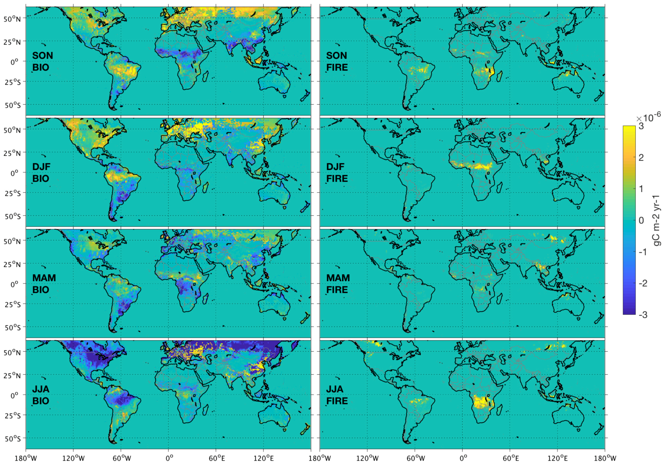
2.2. CarbonTracker CO2 Fluxes

In order to better understand the spatio-temporal patterns in the XCO2 anomaly distribution, we compare our results to NOAA’s CarbonTracker flux maps (see also https://www.esrl.noaa.gov/gmd/ccgg/carbontracker/fluxes.php), version CT2017 ([24] with updates documented at http://carbontracker.noaa.gov). In particular, we consider the biospheric fluxes as well as those associated with biomass burning emissions. As input information, CT2017 uses Global Fire Emissions Database (GFED) 4.1, which is based on MODIS (Moderate Resolution Imaging Spectroradiometer) observations of fire counts. The a priori biospheric fluxes are based on the Carnegie–Ames Stanford Approach (CASA) biogeochemical model, and their scaling factors are estimated using CT2017.

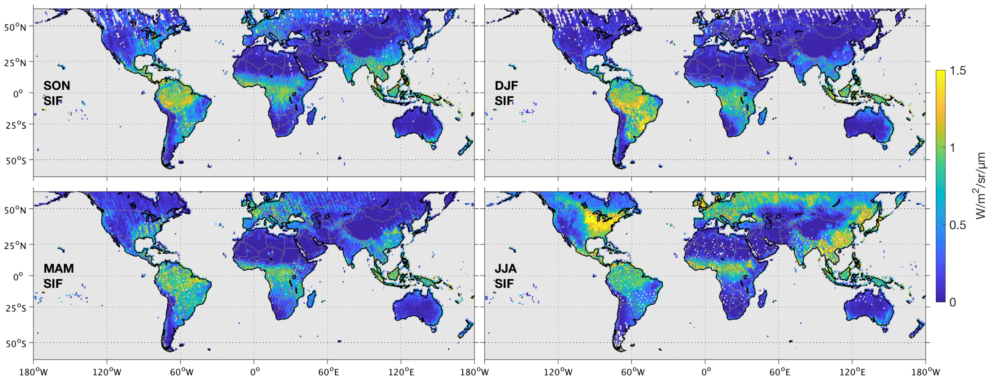
2.3. Solar-Induced Chlorophyll Fluorescence (SIF)

We analyze the solar-induced chlorophyll fluorescence, which is also measured by the OCO-2 instrument [25] at 757 nm and 772 nm. We use the cloud-filtered 757 nm data from the OCO-2 lite files V8r that include quality filtering and bias correction. SIF can serve as a proxy for the vegetation gross primary production (GPP) [26], defined as the synthesis of organic compounds from atmospheric CO2 and principally occurring through the process of photosynthesis. Therefore, SIF data are expected to provide information on the contribution of the CO2 uptake by the vegetation on the XCO2 anomalies.

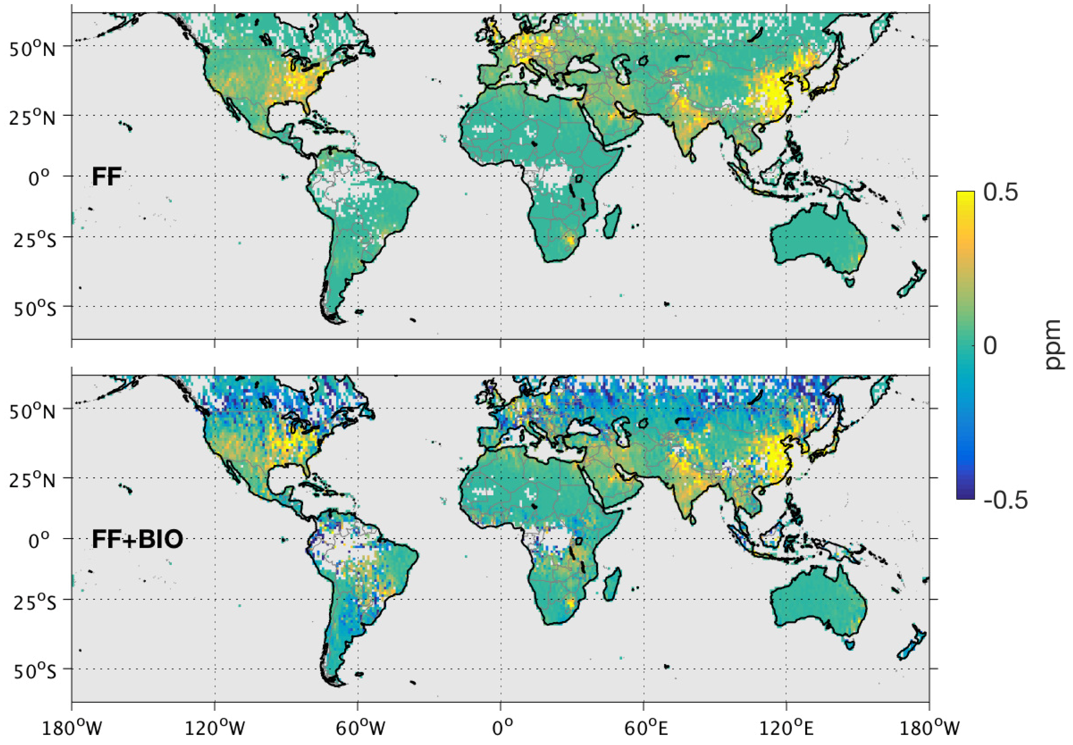
2.4. XCO2 Enhancements from FLEXPART Model

We use the Lagrangian particle dispersion model, FLEXPART (FLEXible PARTicle dispersion model) [27], to simulate anthropogenic and biospheric XCO2 enhancements at OCO-2 measurement locations. We follow the approach used by Janardanan et al. [13], where the localized GOSAT CO2 enhancements are compared to the inventory-based CO2 estimates using the FLEXPART model outputs. We use the JRA-55 meteorology provided at 60 vertical levels and interpolated to a horizontal resolution of 1.25 degrees. As there are about 85 000 OCO-2 data points per day, for computational reasons, we aggregate OCO-2 data points into one-second averages, taken separately for OCO-2 footprints 1–4 and 5–8 (≤12 soundings in one set, 2 sets per second). The sampling corresponds to the OCO-2 data version V7r.
As input information for anthropogenic emissions, we use the high-resolution ODIAC (Open-Data Inventory for Anthropogenic Carbon dioxide) inventory [28]. In the ODIAC inventory, the anthropogenic CO2 emissions are estimated at 1 km × 1 km resolution given the power plant emissions (intensity and geographical location) and satellite-observed nightlights. In the FLEXPART model simulations, from each aggregated OCO-2 data point, ten thousand virtual particles are released and transported three days backward in time with the three-dimensional wind field using parameterizations for turbulence and convection.

2.5. TROPOMI/S5P NO2 Tropospheric Columns

In order to study local scale emission sources in South Africa, we use the TROPOMI/S5P NO2 tropospheric columns [29,30] collocated with the XCO2 anomalies, as indicators of anthropogenic fossil fuel emissions. Launched in October 2017, TROPOMI on board S5P flies on a sun-synchronous polar orbit satellite with overpass time 13:30 LT. TROPOMI NO2 data are publicly available since July 2018 with a spatial resolution of 3.5 km × 7 km at nadir and daily global coverage.

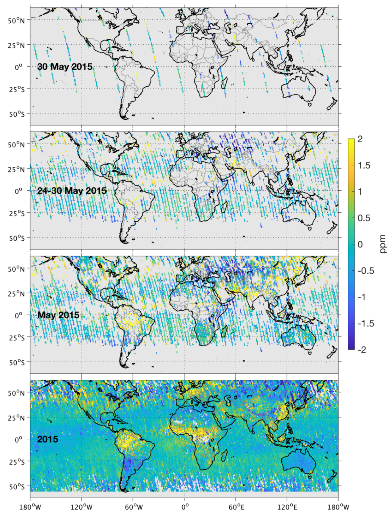
3. Global XCO2 Anomalies

CO2 has a long atmospheric lifetime and relatively large background concentrations (~410 ppm). Because of this, XCO2 varies by only about 2% from pole-to-pole and over the seasonal cycle. Meanwhile, XCO2 variations corresponding to anthropogenic sources are even smaller on the scale of the satellite sounding (2–4 km2). High precision is therefore essential to quantify XCO2 anomalies associated with these sources. Methods like those used to map short-lived air pollutants, like NO2, based on averaging out the outflow downwind from the emission sources, cannot be directly applied to space-based CO2 measurements. The large CO2 background and seasonal variability must be removed before being able to highlight the emission areas.
In order to extract information about the anthropogenic and biogenic signatures from OCO-2 retrievals, we use the concept of XCO2 anomaly [21], defined as the difference between the individual XCO2 value measured by OCO-2 and the daily background:
XCO 2 ( anomaly ) = XCO 2 ( individual ) XCO 2 ( daily background ) .
This equation provides an anomaly value for each OCO-2 data point. Using the daily background allows us to remove the seasonal variability and the increasing trend of CO2 concentrations. Once we obtain the anomalies for each OCO-2 measurement point, we define a spatial grid (e.g., 1° × 1°, latitude-longitude) and calculate the mean at each grid point over a defined period of time. Figure 1 shows examples of mean XCO2 anomalies for one day, one week, one month and one year. The resulting anomaly maps illustrate the areas where CO2 is emitted (positive anomalies) into the atmosphere and those acting as sinks, where CO2 is absorbed at the surface (negative anomalies). The strength of this approach is that it only uses satellite-based measurements and is not dependent on patterns in a priori fields, external data or other assumptions in atmospheric chemistry-transport models.
Defining the area over which the daily background is calculated, is a critical step in the analysis. In [21], we focused on three selected anthropogenic emission areas: (1) North America, (2) Europe, northern Africa, and Middle East, and (3) East Asia. In this paper, our aim is to obtain comparable anomalies for different regions. In order to obtain the background, we calculate the daily medians for each 10-degree latitude band and linearly interpolate the resulting values to each OCO-2 data point. The median was chosen because it better represents the typical value in each latitude band, and it is not skewed towards extreme values.
Figure 2 shows the daily XCO2 background as a function of latitude interpolated at 1-degree resolution. The interpolation step removes the sharp latitudinal boundaries that would result if the daily medians at different latitude bands were used directly. In particular, we would obtain a sharp boundary between the northern high mid-latitudes (40°N–60°N) and lower latitudes during summer months due to the stronger (and shifted) CO2 uptake. The median XCO2 values for each 10-degree latitude band as well as their latitudinal distribution for selected days between September 2015 and September 2016 are included in Figure S1 (top and bottom panels, respectively). The background used in the calculation of the anomalies changes at different times of the year and over different regions. The peak of the seasonal cycle shifts during the year from the Northern to the Southern hemisphere. Also the amplitude of the seasonal cycle is much larger in the Northern Hemisphere due to the strong seasonal biospheric flux differences. Figure 2 also shows the XCO2 values increasing by about 10 ppm from September 2014 to September 2018. We note that no data are available at high middle-latitudes in autumn-winter when the Sun is too low for a successful XCO2 retrieval. Furthermore, a smaller amount of data is expected over areas frequently covered by clouds or with a large aerosol load.

4. Results

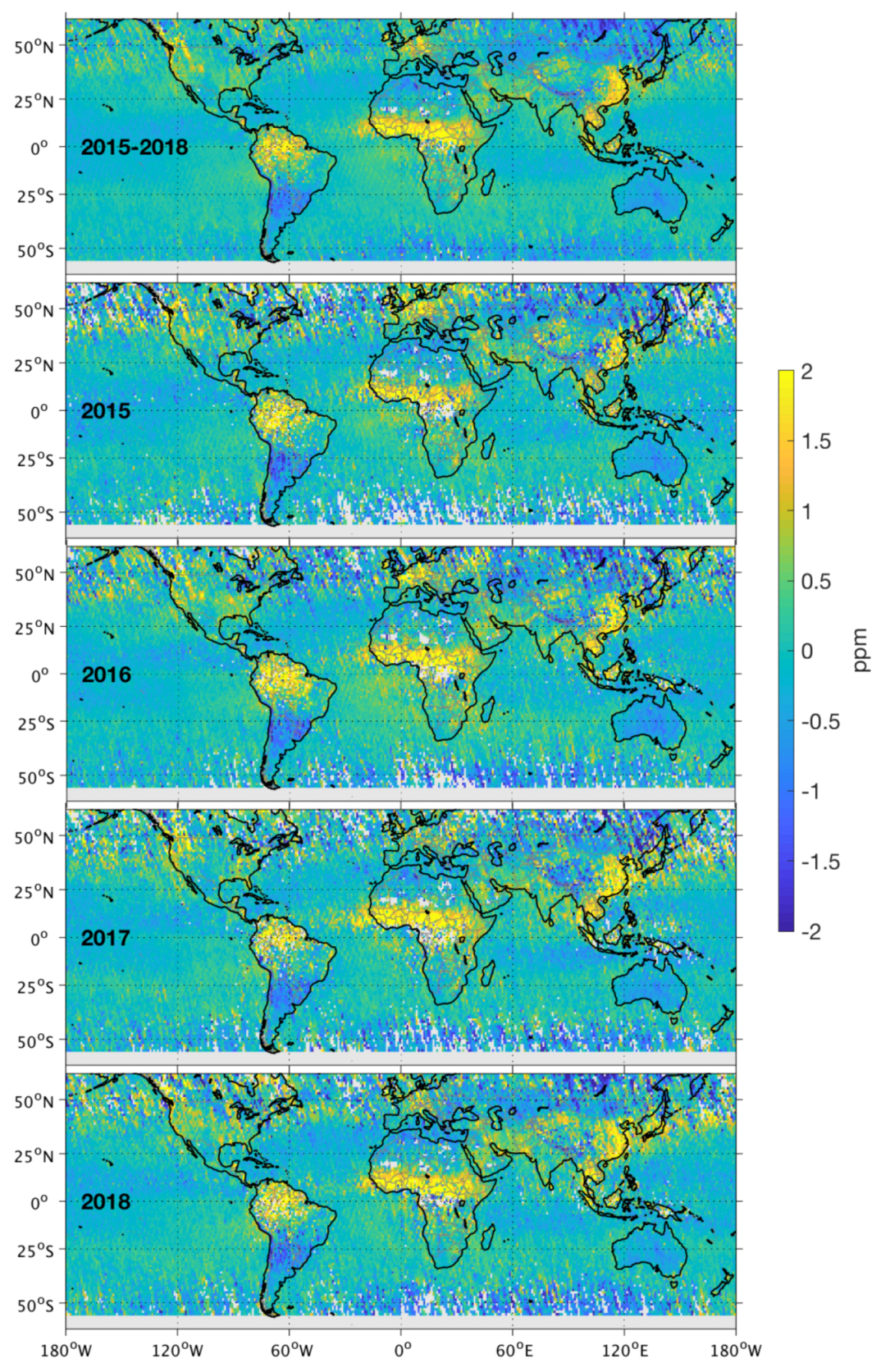
4.1. Annual XCO2 Anomalies

Figure 3 illustrates the mean annual OCO-2 XCO2 anomaly for 2015–2018. The largest anthropogenic anomalies correspond to the areas in China, North-East India, Middle East, central Europe, and eastern USA, as also noted in [21]. In the Southern Hemisphere, the largest anthropogenic emission area, the Highveld region in South Africa, is clearly visible.
The largest positive XCO2 anomalies are observed in the tropical regions in northern and southern Africa, Indonesia, Indochina, and South America. These correspond to large-scale biomass burning and to positive biospheric fluxes (respiration). These anomalies are most intense during the 2015–2016 El Niño, but persist through the four-year period considered here.
The largest negative anomalies are observed in the northern middle-latitudes (40°N–60°N) over Asia and North America. These are clearly associated with the strong biospheric sink during the growing season. This area is mainly sampled by OCO-2 during summer months and not during winter due to persistent cloudiness and low signal levels at high solar zenith angles (see Figure 2). This temporal sampling bias may introduce biases in the annual-average anomalies (examined in greater detail below). We also observe a large area with negative anomalies in the Southern Cone in South America.
The large areas with positive and negative anomalies are quite consistent from year to year. Also, smaller areas with large anomalies seem to be consistently visible in all years (e.g., the Highveld region). Some differences in the XCO2 anomaly patterns between different years are, at least partly, related to the sampling of the instrument and the number of data points available. These are most visible for example at northern and southern mid-latitudes, where we can still identify individual “satellite tracks” from the map. In Figure S2 of the supplementary material, we present the maps of the number of data points that were used to calculate the mean in Figure 3. In addition to northern latitudes, the number of data points is lower also in places with high cloud density and/or large aerosol load (Himalaya, Amazonia, central Africa and China). Thus, the anomalies calculated over these areas are less robust. This is further illustrated in Figure S3, which shows the standard error of the mean, i.e., sample standard deviation divided by the square root of the sample size.
We find that the ocean XCO2 anomalies are ~0.5 ppm lower than those over land. The XCO2 concentrations are generally continuous across coastlines, clearly revealing outflow regions west of tropical Africa, and east of the east coasts of China and the U.S. The low bias over the ocean is generally consistent with the hypothesis that the ocean is a net sink for CO2, absorbing about 8.9 GtCO2/year [31]. However, it is important to note that the approach for defining the background and anomalies adopted here was optimized for identifying point emission sources. It might not be ideal for quantifying weak, spatially extensive sinks, like those expected over ocean and seen in our anomaly plots. For example, Gurney et al. [32] found that the simulations of oceanic CO2 surface concentrations show about 1 ppm variation in the annual zonal mean. Also, the low XCO2 values over the tropical and high latitude ocean are among the most difficult to validate given the lack of TCCON stations at those latitudes and very limited in situ measurements. This is therefore active area of research within the scientific community.

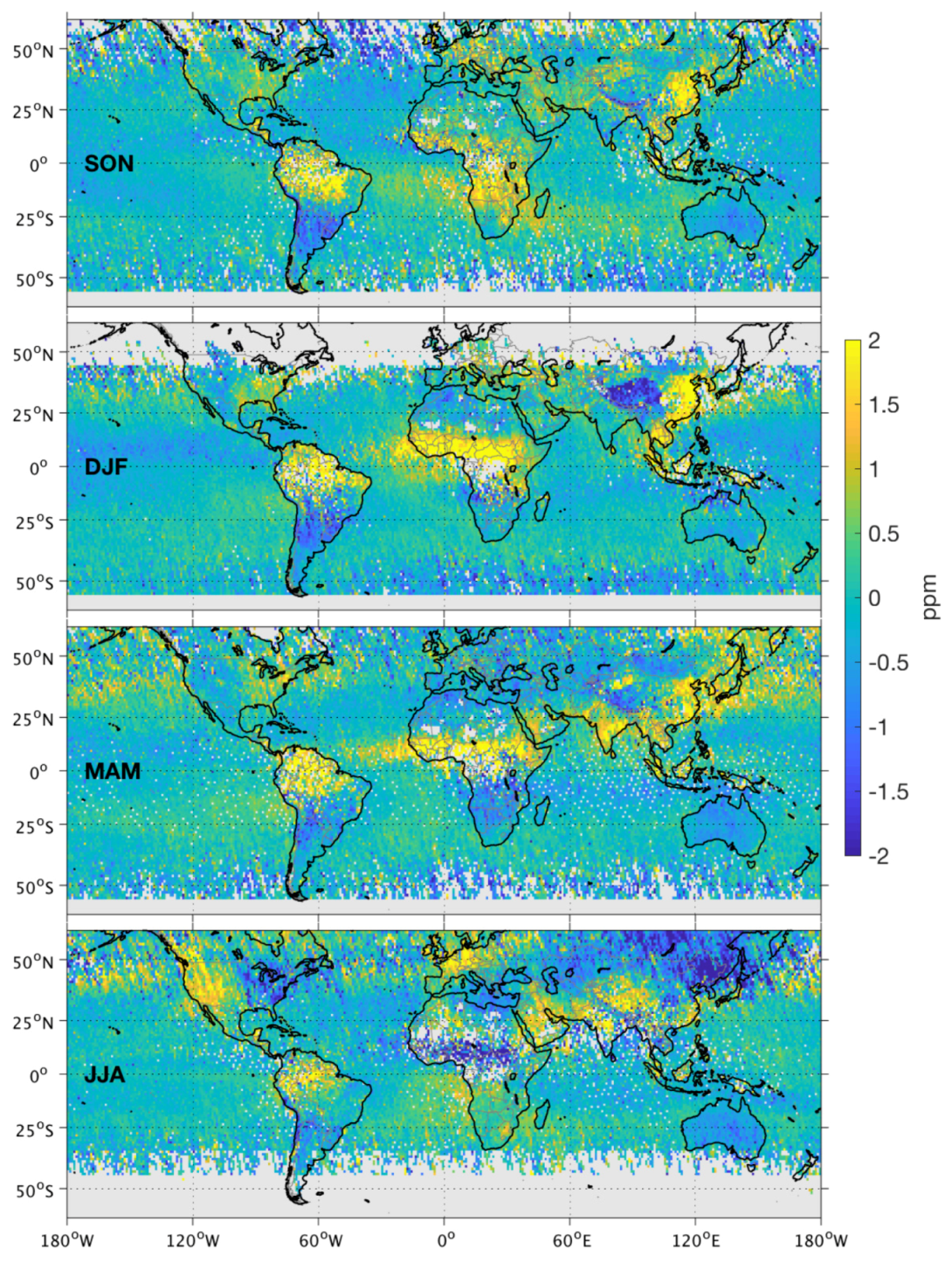
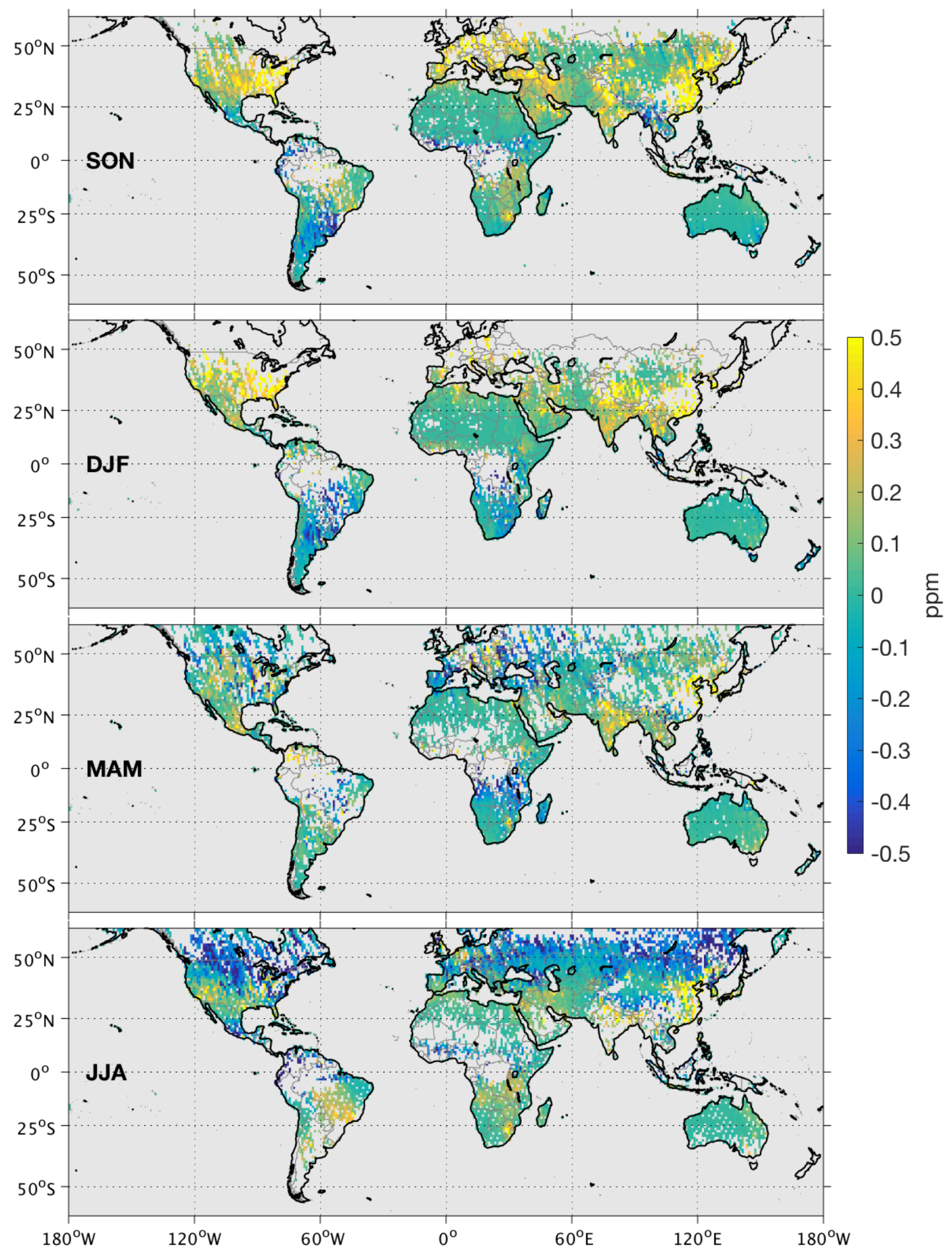
4.2. Seasonal XCO2 Anomalies

Figure 4 illustrates the mean seasonal XCO2 anomalies calculated from the period September 2014 to August 2018. The different seasons are defined as September-October-November (SON), December-January-February (DJF), March-April-May (MAM), and June-July-August (JJA). The large-scale patterns on SON, DJF, MAM look very similar to each other and to the annual mean, while in JJA the anomaly distribution looks quite different, with strong negative anomalies over the Northern Hemispheric mid-latitudes. We note that no OCO-2 observations are available during winter months (DJF) over the northern high- and mid-latitudes, due to persistent cloudiness and low signal levels. Figure S4 in the supplementary material shows the number of data points available for each season from September 2014 to August 2018. The standard error of the mean is illustrated in Figure S5.
In order to better understand this seasonal variability, we analyze the seasonal distribution of the SIF (Figure 5), also measured by OCO-2, as well as the fluxes from NOAA’s CarbonTracker model (Figure 6). Both SIF and CarbonTracker flux spatial distributions show how the negative anomalies observed during JJA are related to the biospheric sink (i.e., high SIF and negative fluxes). This is particularly visible in the eastern part of North America, where the highest SIF values are observed. At the same time, low SIF values and high XCO2 anomalies are observed in the western part of North America. The high XCO2 anomalies observed in part of the northern hemisphere during JJA are partially related to the seasonal minimum of the background (Figure 2 and Figure S1). These patterns, however, do not contradict the patterns in the CarbonTracker flux map and are similar to the seasonal FLEXPART modeling results described in Section 4.3.
The XCO2 anomaly patterns in Africa show positive values in the northern biomass burning area during winter months (DJF) and relatively smaller anomalies during SON and MAM. During summer months, we find mainly negative XCO2 anomalies over the same area. These features correspond directly to those observed in the CarbonTracker flux maps, i.e., strong emissions from biomass burning during winter and uptake during summer (Figure 6, right column). SIF is also higher during summer months, when the XCO2 anomalies are negative. In the southern biomass burning area in Africa, we observe the largest XCO2 anomalies during SON and JJA, when the biomass burning emissions are the strongest (Figure 6, right column) and SIF values relatively small. The largest negative XCO2 anomalies are seen in DJF and MAM, when there are reduced emissions from biomass burning. From Figure 4, we find that the XCO2 anomalies over the Highveld area in South Africa are the largest during JJA and SON, when the CO2 uptake by photosynthesis is minimum.
The limited number of data points available over Amazonia makes the quantification of the XCO2 anomalies in South America more challenging (Figure S4). This is also illustrated in Figure S5 with high values of the standard error of the mean. The XCO2 anomaly values are positive throughout the year, although, smaller anomalies are observed in JJA when the biospheric fluxes are negative. Signatures from biomass burning and positive biospheric fluxes are visible as larger positive anomalies during SON. In the Southern Cone, the XCO2 anomalies are most negative during SON and DJF, which is in line with the SIF and biospheric flux maps, indicating that these anomalies are primarily biogenic.
In Indochina, negative XCO2 anomalies correspond to the largest SIF values observed during JJA, although from the biospheric flux maps, we would expect positive fluxes during JJA. During DJF and MAM, we see the signature of strong emission from fires in the anomalies and flux maps (Figure 6, right column). We would expect however to see negative anomalies during SON due to the strong biospheric sink, but we find only slightly smaller positive anomalies. In the Indian peninsula we find positive XCO2 anomalies as expected from anthropogenic emissions when the biospheric uptake is low.
Seasonal patterns are also evident in the largest anthropogenic emission areas, i.e., China, central Europe and eastern USA. For example, China and central Europe show positive anomalies during all seasons, while in eastern USA these are offset by a very strong biospheric sink in JJA. Also, the positive XCO2 anomalies in China and central Europe are lower during JJA and MAM, respectively. Arid and semi-arid regions, including the Sahara, Tibetan Plateau and Australia, are out of sync with the rest of their hemispheres, with negative anomalies in the winter and small positive anomalies in the summer.
Finally, we note signatures of outflow over the Atlantic ocean with positive XCO2 anomalies from the biomass burning emissions in Africa. Furthermore, the spring time outflow along the dominant westerlies from China to North America is also visible from Figure 4, as also observed, e.g., for tropospheric ozone in several studies (e.g., [33,34]).

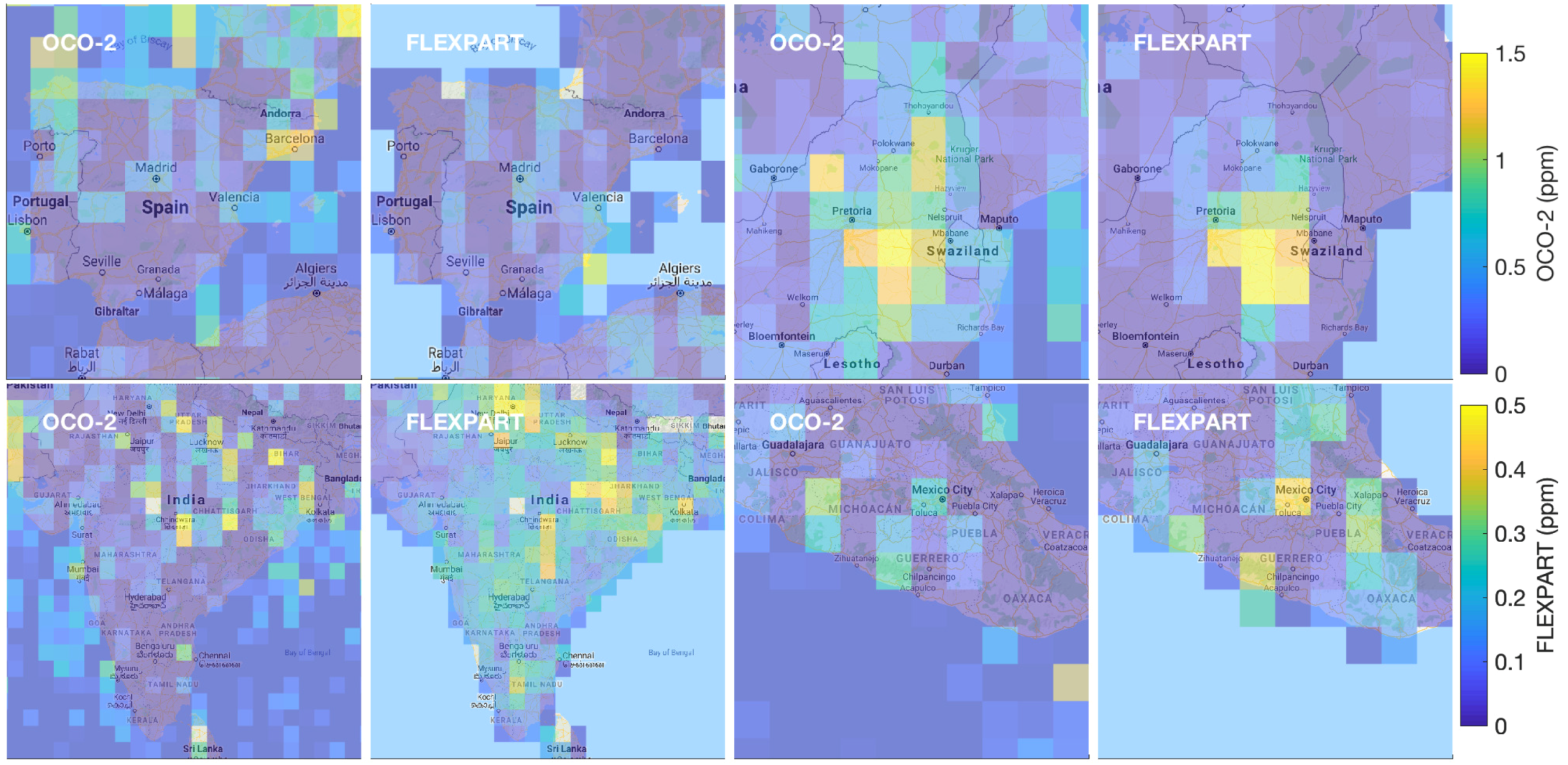
4.3. Modeling Results

We analyze the XCO2 enhancements related to fossil fuel combustion and biospheric fluxes corresponding to the OCO-2 sounding footprints using the Lagrangian FLEXPART model. This allows us to account for the effect of the OCO-2 sampling as well as the transport by the wind.
Figure 7 illustrates the modeled XCO2 enhancements for the year 2015. We illustrate the contribution from the ODIAC fossil fuel fluxes alone (Figure 7, upper panel) and together with the biospheric contribution (Figure 7, lower panel). The anthropogenic component shows spatial patterns similar to those observed from the XCO2 anomalies in Figure 3, with high positive enhancements in eastern USA, Europe, India, Middle East and China. In the Southern Hemisphere, the Highveld region in South Africa shows the strongest anthropogenic signal, together with the area around Sidney in Australia. When adding the biospheric component, we also find negative values in the northern mid-latitudes and in the Southern Cone in South America, as observed from the anomalies in Figure 3. In Europe, the large anthropogenic XCO2 enhancements are drawn down by the biospheric sink (Figure 7, lower panel). The largest differences between the patterns in the FLEXPART simulations and the OCO-2 anomalies are in the tropical region, where the OCO-2 XCO2 anomalies show large positive values while the FLEXPART enhancements are close to zero. Part of the reason is that the FLEXPART simulations do not include the biomass burning contribution, but also the biospheric contribution is lower.
Figure 8 illustrates the results of the FLEXPART seasonal simulations. We find that the Highveld region is clearly visible during SON and JJA, while it is not detectable during DJF due to effect of the biospheric sink. The same feature is also visible in the seasonal anomalies in Figure 4. In addition, while OCO-2 shows negative XCO2 anomalies over central North America and South Central Asia during the fall (SON) and winter (DJF), the FLEXPART enhancements over both regions are positive.
Four local “case studies” for both FLEXPART enhancements and OCO-2 anomalies are illustrated in Figure 9. The first one is the Iberian peninsula, where OCO-2 XCO2 retrievals are available consistently throughout the year. Here, OCO-2 measurements indicate larger XCO2 anomalies over coastal cities than the model results. The second area is the Highveld industrial region in South Africa. In this case, the anthropogenic signatures seem more localized in the FLEXPART simulations than in the OCO-2 anomaly maps, although positive anomalies are clearly visible over the area as well. The third case study is over India, where we can see a clear positive signal in both OCO-2 and FLEXPART data, but the OCO-2 results indicate more discrete and localized anthropogenic emissions than the model results. The last case is Mexico City, where we also see strong anthropogenic signatures (i.e., positive enhancements and anomalies), related to the emissions from the city as well as the power plants in the area, with some differences in the locations of the positive enhancements. These differences may reflect uncertainties in the the emission source intensities or locations or significant local wind data errors at low wind conditions while using wind data from global reanalysis.

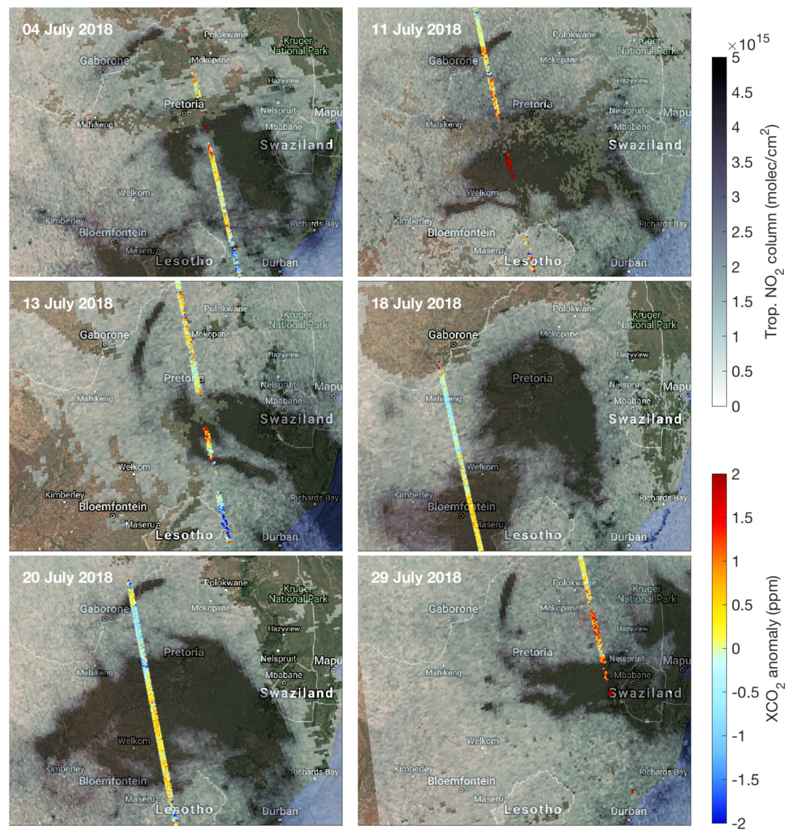
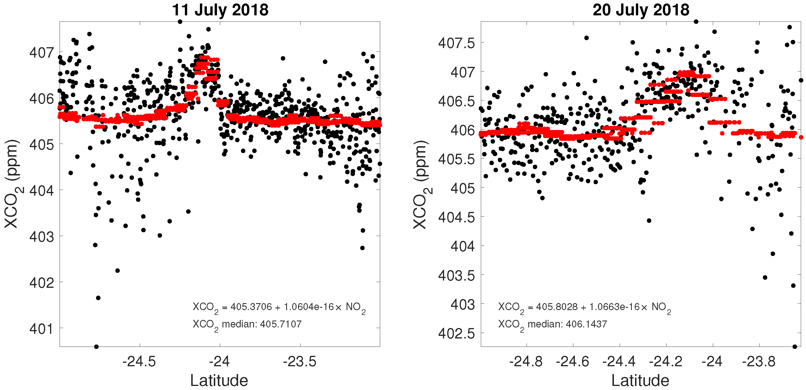
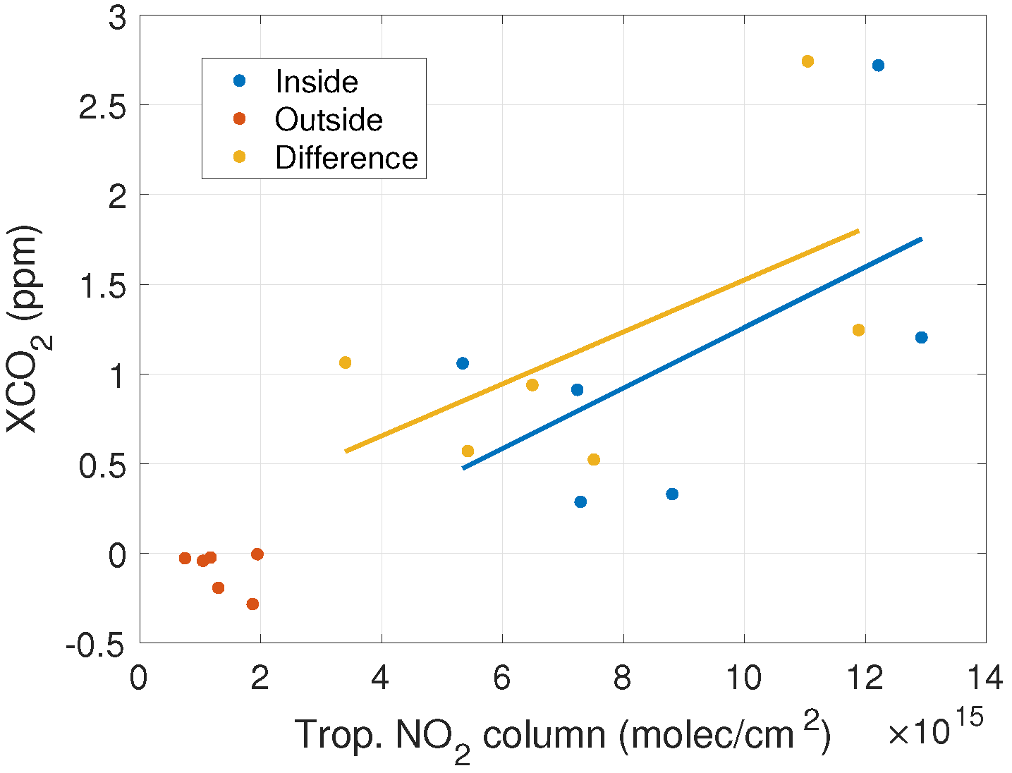
4.4. Case Study: Collocated OCO-2 and TROPOMI Observations in the Highveld Region

We analyse the daily XCO2 anomalies over the Highveld industrial region in South Africa together with NO2 tropospheric columns. The area includes several coal-fired power plants as well as pollution from urban sites. We concentrate the analysis on the month of July 2018, in order to reduce the effect of the CO2 drawdown. We find six direct overlaps with the OCO-2 swath (including a sufficient number of XCO2 retrievals) passing through NO2 local enhancements (plumes). In Figure 10, we illustrate the TROPOMI NO2 tropospheric columns overlaid with local OCO-2 XCO2 anomalies (with background calculated from the values inside a latitude-longitude box [40°S, 20°S] × [15°E, 45°E]). In all six cases, we note clear XCO2 gradients between the area inside the NO2 plume and the surrounding background. On 11 and 20 July 2018, we identify smaller plumes originating from Matimba coal-fired power plant, but also on 13 July 2018 we see fine structures with high XCO2 anomalies over the NO2 plumes.
In order to analyze the cases further, we collocate the TROPOMI NO2 observations to each OCO-2 footprint. In Figure S6, we illustrate the normalized histograms of OCO-2 XCO2 anomalies labeled as “anthropogenic” and “surrounding,” discriminated when tropospheric NO2 values are larger or smaller than 5 × 10 15 molec./cm2, respectively. In all cases, we note that the anthropogenic histograms peak at higher positive XCO2 anomalies than the histogram for the surrounding. We also note that on 4 July 2018, only a few data points are classified as “anthropogenic”. In Figure 11, we illustrate the correlation between the median NO2 and XCO2 anomaly values inside and outside the NO2 plume as well as the difference between the values inside and outside the plume for each of the six days. We note that the points outside the NO2 plumes (red dots in Figure 11) fall into the bottom-left part of the scatter plot, corresponding to negative XCO2 anomalies and relatively low NO2 levels. Meanwhile, the points falling inside the plume with enhanced NO2 levels (blue dots in Figure 11) show a positive linear correlation between the median NO2 tropospheric columns and XCO2 anomalies. A similar correlation is observed for the differences between the values inside and outside the plume (yellow dots in Figure 11). In both cases, the slope, or the CO2-to-NO2 ratio, is about ~1.5 × 10 16 ppm/(molec./cm2). On 11 and 20 July 2018, the OCO-2 flight track passes right through the NO2 plume generated from the Matimba power plant. Figure 12 shows the OCO-2 XCO2 values (black dots) as a function of latitude during both days. Figure 12 (red dots) also includes the XCO2 values obtained by empirically converting TROPOMI NO2 tropospheric columns (collocated to the OCO-2 measurements) into XCO2 using the results of the linear regression between the two data sets. The CO2-to-NO2 ratio in both days was found to be ~1.1 × 10 16 ppm/(molec./cm2). Both XCO2 cross-sections show a similar enhancement when passing through the emission plumes (latitude 24.1°S).

5. Discussion

Current CO2 missions have been primarily designed to extend the spatial coverage of the ground-based atmospheric observation networks and to improve the model estimates of biospheric fluxes on regional scale. The COP 21 Paris agreement emphasizes the need to monitor anthropogenic CO2 emissions over a range of scales [35]. The anomaly approach presented here exploits the intrinsic value and capabilities of satellite-based CO2 observations for mapping anthropogenic and natural emission patterns, beyond their application as model input information. The observed consistency between satellite-based XCO2 anomalies and model outputs (distinguishing fossil fuel and biospheric contributions) demonstrates the capability of satellite observations for describing the CO2 spatio-temporal variability and, in particular, for detecting anthropogenic CO2 emission patterns.
A feature of the anomaly approach is that the XCO2 anomalies (given in ppms) are not directly convertible to fluxes (given in ktons/day). The approach often taken with short-lived air pollutants is to use a statistical model that describes their spatial distribution near the emission sources as a function of wind speed and direction (e.g., [36,37]). In the future, a similar approach might also be possible with XCO2 anomalies, for example using CO2 measuring satellites with wider swaths, such as the anthropogenic CO2 monitoring satellite constellation planned by the European Copernicus Programme. In this context, the results presented here highlight the need for satellite observations with high precision, good accuracy and dense sampling covering a wider swath (e.g., few hundred km) than OCO-2, in order to separate individual emission sources (e.g., cities or large power plants) from the background signal. Here we showed how overlapping OCO-2 XCO2 data and TROPOMI NO2 observations (covering a large swath) can be used to identify small scale anthropogenic CO2 signatures.
The anomaly approach is also a useful tool for identifying CO2 fluxes associated with the natural carbon cycle. For example, the XCO2 anomaly maps show persistent positive XCO2 anomalies (1–2 ppm) over the Amazon, Congo, and tropical Oceania. The intensity and spatial extent of the positive XCO2 anomaly is largest during the 2015–2016 El Niño, but it spanned every season of every year included in this study. This appears to support the conclusions of Baccini et al. [38] who assert that the tropical deforestation and degradation have compromised these forests to the extent that they are now net sources instead of sinks of carbon, even if this conclusion is still under debate [39]. A recent study by Pugh et al. [40] also indicates that contrary to previous findings, the sink is predominantly in mid-high latitude, rather than tropical, forests.
The method presented here can also be applied to future planned XCO2 missions, such as OCO-3, GOSAT-2, MicroCarb, GeoCarb, and the Chinese and European wide-swath constellations. The global approach can be easily applied to instruments that fly in near-polar, sun-synchronous orbits, however, adjustments to background definition are needed for instruments operating on the International Space Station (e.g., OCO-3) or on geostationary orbit (e.g., GeoCarb) due to the possible influence of diurnal variations and spatial coverage. Further applications of this method could combine anomalies from similar platforms, e.g. belonging to the same constellation.

6. Conclusions

In this paper, we analyzed four years (2015–2018) of Orbiting Carbon Observatory-2 (OCO-2) data to derive global (60°S–60°N) XCO2 anomalies. We calculated regional-scale XCO2 anomalies and identified the main anthropogenic emission areas, biomass burning regions, and biospheric sinks. We find that the patterns observed in OCO-2 annual XCO2 anomalies are robust and consistent from year-to-year. From the seasonal XCO2 anomalies, we identified the patterns in the Northern Hemispheric growing season and also the different fire seasons in Africa. In addition to large-scale features, we also visualized different local “case studies” with high anomalies associated with anthropogenic emissions in both the Northern and Southern Hemispheres. Finally, we combined daily XCO2 anomalies with TROPOspheric Monitoring Instrument (TROPOMI) NO2 tropospheric columns, used as an indicator of anthropogenic pollution plumes, over the Highvelt industrial region in South Africa. We find corresponding gradients and positive correlation between XCO2 anomalies and NO2 enhancements.
From a methodological point of view, instrument sampling, background choice, and bias correction do have an impact on the OCO-2 XCO2 anomaly patterns. Thus, the results are most significant over areas where more data are available throughout the year. The consistency of the spatial features from year to year (or for the same season during different years) is an indicator of the robustness of the results. The FLEXible PARTicle dispersion model (FLEXPART) simulations also confirm the observed spatial patterns. On the other hand, the error associated with the anomaly is not purely statistical and tends to be more systematic due to errors in assumed source location, intensity, persistent wind patterns, and uneven geographic distribution of OCO-2 observations. For example, OCO-2 data in the northern high- and middle-latitudes are available predominantly during summer months so the annual maps are likely to be biased towards the anomalies derived during this period.
We showed that using a piecewise linear background for the calculation of the anomalies provides a robust tool for global analysis. We have tested different background choices, as well as different OCO-2 data versions (V7r, V8r). We conclude that the structure and amplitude of the anomalies is relatively insensitive to these choices, although, for example, using narrow latitude bands without interpolation would yield sharp latitudinal boundaries in the maps. When analyzing local case studies on regional scales, a different background region can be selected, as shown for example in the South Africa’s case study (Section 4.4) or by Wang et al. [17] in China.

Supplementary Materials

The following are available online at https://www.mdpi.com/2072-4292/11/7/850/s1, Figure S1: OCO-2 seasonal cycle at 10 degree latitude bands and latitudinal gradient at selected days between September 2015 and September 2016, Figure S2: Number of data points on each 1° × 1° grid cell, Figure S3: Standard error of the mean on each 1° × 1° grid cell, Figure S4: Number of data points on each 1° × 1° grid cell at each season from September 2014 to August 2018, Figure S5: Standard error of the mean for the seasonal XCO2 anomalies 2014–2018, Figure S6: Histograms of XCO2 anomalies inside and outside the NO2 plumes.

Author Contributions

J.H. and I.I. analyzed the data and wrote the first draft of the manuscript. S.M. and D.C. provided data and expertise on FLEXPART and OCO-2, respectively, and helped in finalizing the paper.

Funding

Janne Hakkarainen and Iolanda Ialongo acknowledge the funding from the European Space Agency (DACES project), and the Academy of Finland, project numbers 312125 and 303876, respectively. Shamil Maksyutov is supported by the GOSAT project. The contributions from David Crisp were conducted at the Jet Propulsion Laboratory, California Institute of Technology, under a contract with the National Aeronautics and Space Administration.

Acknowledgments

The authors would like to acknowledge all the parties that provided open-access data. OCO-2 data can be downloaded using the MIRADOR platform (http://mirador.gsfc.nasa.gov). TROPOMI data can be downloaded from Sentinel-5P Pre-Operations Data Hub (https://s5phub.copernicus.eu/dhus/). CarbonTracker CT2017 results provided by NOAA ESRL, Boulder, Colorado, USA from the website at http://carbontracker.noaa.gov. FLEXPART model simulation can be obtained from Shamil Maksyutov ([email protected]). ODIAC fossil fuel CO2 emissions dataset is available from http://db.cger.nies.go.jp/dataset/ODIAC/.

Conflicts of Interest

The authors declare no conflict of interest.

References

  1. Eldering, A.; O’Dell, C.W.; Wennberg, P.O.; Crisp, D.; Gunson, M.R.; Viatte, C.; Avis, C.; Braverman, A.; Castano, R.; Chang, A.; et al. The Orbiting Carbon Observatory-2: First 18 months of science data products. Atmos. Meas. Tech. 2017, 10, 549–563. [Google Scholar] [CrossRef]
  2. Eldering, A.; Wennberg, P.O.; Crisp, D.; Schimel, D.S.; Gunson, M.R.; Chatterjee, A.; Liu, J.; Schwandner, F.M.; Sun, Y.; O’Dell, C.W.; et al. The Orbiting Carbon Observatory-2 early science investigations of regional carbon dioxide fluxes. Science 2017, 358. [Google Scholar] [CrossRef]
  3. Varon, D.J.; Jacob, D.J.; McKeever, J.; Jervis, D.; Durak, B.O.A.; Xia, Y.; Huang, Y. Quantifying methane point sources from fine-scale satellite observations of atmospheric methane plumes. Atmos. Meas. Tech. 2018, 11, 5673–5686. [Google Scholar] [CrossRef]
  4. Chevallier, F.; Bréon, F.M.; Rayner, P.J. Contribution of the Orbiting Carbon Observatory to the estimation of CO2 sources and sinks: Theoretical study in a variational data assimilation framework. J. Geophys. Res. Atmos. 2007, 112. [Google Scholar] [CrossRef]
  5. Miller, C.E.; Crisp, D.; DeCola, P.L.; Olsen, S.C.; Randerson, J.T.; Michalak, A.M.; Alkhaled, A.; Rayner, P.; Jacob, D.J.; Suntharalingam, P.; et al. Precision requirements for space-based data. J. Geophys. Res. Atmos. 2007, 112. [Google Scholar] [CrossRef]
  6. Burrows, J.; Hölzle, E.; Goede, A.; Visser, H.; Fricke, W. SCIAMACHY—Scanning imaging absorption spectrometer for atmospheric chartography. Acta Astronaut. 1995, 35, 445–451. [Google Scholar] [CrossRef]
  7. Yokota, T.; Yoshida, Y.; Eguchi, N.; Ota, Y.; Tanaka, T.; Watanabe, H.; Maksyutov, S. Global Concentrations of CO2 and CH4 Retrieved from GOSAT: First Preliminary Results. SOLA 2009, 5, 160–163. [Google Scholar] [CrossRef]
  8. Crisp, D.; Pollock, H.R.; Rosenberg, R.; Chapsky, L.; Lee, R.A.M.; Oyafuso, F.A.; Frankenberg, C.; O’Dell, C.W.; Bruegge, C.J.; Doran, G.B.; et al. The on-orbit performance of the Orbiting Carbon Observatory-2 (OCO-2) instrument and its radiometrically calibrated products. Atmos. Meas. Tech. 2017, 10, 59–81. [Google Scholar] [CrossRef]
  9. Yang, D.; Liu, Y.; Cai, Z.; Chen, X.; Yao, L.; Lu, D. First Global Carbon Dioxide Maps Produced from TanSat Measurements. Adv. Atmos. Sci. 2018, 35, 621–623. [Google Scholar] [CrossRef]
  10. Cai, Z.; Liu, Y.; Yang, D. Analysis of CO2 retrieval sensitivity using simulated Chinese Carbon Satellite (TanSat) measurements. Sci. China Earth Sci. 2014, 57, 1919–1928. [Google Scholar] [CrossRef]
  11. Nassar, R.; Hill, T.G.; McLinden, C.A.; Wunch, D.; Jones, D.B.A.; Crisp, D. Quantifying CO2 Emissions From Individual Power Plants From Space. Geophys. Res. Lett. 2017, 44, 10045–10053. [Google Scholar] [CrossRef]
  12. Reuter, M.; Buchwitz, M.; Hilboll, A.; Richter, A.; Schneising, O.; Hilker, M.; Heymann, J.; Bovensmann, H.; Burrows, J.P. Decreasing emissions of NOx relative to CO2 in East Asia inferred from satellite observations. Nat. Geosci. 2014, 7, 792. [Google Scholar] [CrossRef]
  13. Janardanan, R.; Maksyutov, S.; Oda, T.; Saito, M.; Kaiser, J.W.; Ganshin, A.; Stohl, A.; Matsunaga, T.; Yoshida, Y.; Yokota, T. Comparing GOSAT observations of localized CO2 enhancements by large emitters with inventory-based estimates. Geophys. Res. Lett. 2016, 43, 3486–3493. [Google Scholar] [CrossRef]
  14. Kort, E.A.; Frankenberg, C.; Miller, C.E.; Oda, T. Space-based observations of megacity carbon dioxide. Geophys. Res. Lett. 2012, 39. [Google Scholar] [CrossRef]
  15. Schwandner, F.M.; Gunson, M.R.; Miller, C.E.; Carn, S.A.; Eldering, A.; Krings, T.; Verhulst, K.R.; Schimel, D.S.; Nguyen, H.M.; Crisp, D.; et al. Spaceborne detection of localized carbon dioxide sources. Science 2017, 358. [Google Scholar] [CrossRef] [PubMed]
  16. Ye, X.; Lauvaux, T.; Kort, E.A.; Oda, T.; Feng, S.; Lin, J.C.; Yang, E.; Wu, D. Constraining fossil fuel CO2 emissions from urban area using OCO-2 observations of total column CO2. Atmos. Chem. Phys. Discuss. 2017, 2017, 1–30. [Google Scholar] [CrossRef]
  17. Wang, S.; Zhang, Y.; Hakkarainen, J.; Ju, W.; Liu, Y.; Jiang, F.; He, W. Distinguishing anthropogenic CO2 emissions from different energy intensive industrial sources using OCO-2 observations: A case study in northern China. J. Geophys. Res. Atmos. 2018, 123, 9462–9473. [Google Scholar] [CrossRef]
  18. Wunch, D.; Wennberg, P.O.; Osterman, G.; Fisher, B.; Naylor, B.; Roehl, C.M.; O’Dell, C.; Mandrake, L.; Viatte, C.; Kiel, M.; et al. Comparisons of the Orbiting Carbon Observatory-2 (OCO-2) XCO2 measurements with TCCON. Atmos. Meas. Tech. 2017, 10, 2209–2238. [Google Scholar] [CrossRef]
  19. Liu, J.; Bowman, K.W.; Schimel, D.S.; Parazoo, N.C.; Jiang, Z.; Lee, M.; Bloom, A.A.; Wunch, D.; Frankenberg, C.; Sun, Y.; et al. Contrasting carbon cycle responses of the tropical continents to the 2015–2016 El Niño. Science 2017, 358. [Google Scholar] [CrossRef]
  20. Houweling, S.; Baker, D.; Basu, S.; Boesch, H.; Butz, A.; Chevallier, F.; Deng, F.; Dlugokencky, E.J.; Feng, L.; Ganshin, A.; et al. An intercomparison of inverse models for estimating sources and sinks of CO2 using GOSAT measurements. J. Geophys. Res. Atmos. 2015, 120, 5253–5266. [Google Scholar] [CrossRef]
  21. Hakkarainen, J.; Ialongo, I.; Tamminen, J. Direct space-based observations of anthropogenic CO2 emission areas from OCO-2. Geophys. Res. Lett. 2016, 43, 11400–11406. [Google Scholar] [CrossRef]
  22. O’Dell, C.W.; Eldering, A.; Wennberg, P.O.; Crisp, D.; Gunson, M.R.; Fisher, B.; Frankenberg, C.; Kiel, M.; Lindqvist, H.; Mandrake, L.; et al. Improved retrievals of carbon dioxide from Orbiting Carbon Observatory-2 with the version 8 ACOS algorithm. Atmos. Meas. Tech. 2018, 11, 6539–6576. [Google Scholar] [CrossRef]
  23. Kiel, M.; O’Dell, C.W.; Fisher, B.; Eldering, A.; Nassar, R.; MacDonald, C.G.; Wennberg, P.O. How bias correction goes wrong: Measurement of XCO2 affected by erroneous surface pressure estimates. Atmos. Meas. Tech. Discuss. 2018, 2018, 1–38. [Google Scholar] [CrossRef]
  24. Peters, W.; Jacobson, A.R.; Sweeney, C.; Andrews, A.E.; Conway, T.J.; Masarie, K.; Miller, J.B.; Bruhwiler, L.M.P.; Pétron, G.; Hirsch, A.I.; et al. An atmospheric perspective on North American carbon dioxide exchange: CarbonTracker. Proc. Natl. Acad. Sci. USA 2007, 104, 18925–18930. [Google Scholar] [CrossRef]
  25. Frankenberg, C.; O’Dell, C.; Berry, J.; Guanter, L.; Joiner, J.; Köhler, P.; Pollock, R.; Taylor, T.E. Prospects for chlorophyll fluorescence remote sensing from the Orbiting Carbon Observatory-2. Remote Sens. Environ. 2014, 147, 1–12. [Google Scholar] [CrossRef]
  26. Sun, Y.; Frankenberg, C.; Wood, J.D.; Schimel, D.S.; Jung, M.; Guanter, L.; Drewry, D.T.; Verma, M.; Porcar-Castell, A.; Griffis, T.J.; et al. OCO-2 advances photosynthesis observation from space via solar-induced chlorophyll fluorescence. Science 2017, 358. [Google Scholar] [CrossRef]
  27. Stohl, A.; Forster, C.; Frank, A.; Seibert, P.; Wotawa, G. Technical note: The Lagrangian particle dispersion model FLEXPART version 6.2. Atmos. Chem. Phys. 2005, 5, 2461–2474. [Google Scholar] [CrossRef]
  28. Oda, T.; Maksyutov, S.; Andres, R.J. The Open-source Data Inventory for Anthropogenic CO2, version 2016 (ODIAC2016): A global monthly fossil fuel CO2 gridded emissions data product for tracer transport simulations and surface flux inversions. Earth Syst. Sci. Data 2018, 10, 87–107. [Google Scholar] [CrossRef]
  29. Eskes, H.; van Geffen, J.; Boersma, F.; Eichmann, K.U.; Apituley, A.; Pedergnana, M.; Sneep, M.; Veefkind, J.P.; Loyola, D. Sentinel-5 precursor/TROPOMI Level 2 Product User Manual Nitrogendioxide; Technical Report S5P-KNMI-L2-0021-MA; CI-7570-PUM, issue 2.0.0; Koninklijk Nederlands Meteorologisch Instituut (KNMI): De Bilt, The Nederlands, 2018.
  30. Veefkind, J.P.; Aben, I.; McMullan, K.; Forster, H.; de Vries, J.; Otter, G.; Claas, J.; Eskes, H.J.; de Haan, J.F.; Kleipool, Q.; et al. TROPOMI on the ESA Sentinel-5 Precursor: A GMES mission for global observations of the atmospheric composition for climate, air quality and ozone layer applications. Remote Sens. Environ. 2012, 120, 70–83. [Google Scholar] [CrossRef]
  31. Le Quéré, C.; Andrew, R.M.; Friedlingstein, P.; Sitch, S.; Hauck, J.; Pongratz, J.; Pickers, P.A.; Korsbakken, J.I.; Peters, G.P.; Canadell, J.G.; et al. Global Carbon Budget 2018. Earth Syst. Sci. Data 2018, 10, 2141–2194. [Google Scholar] [CrossRef]
  32. Gurney, K.; Law, R.; Denning, A.; Rayner, P.; Baker, D.; Bousquet, P.; Bruhwiler, L.; Chen, Y.; Ciais, P.; Fan, S.; et al. TransCom 3 CO2 inversion intercomparison: 1. Annual mean control results and sensitivity to transport and prior flux information. Tellus B 2003, 55, 555–579. [Google Scholar] [CrossRef]
  33. Verstraeten, W.W.; Neu, J.L.; Williams, J.E.; Bowman, K.W.; Worden, J.R.; Boersma, K.F. Rapid increases in tropospheric ozone production and export from China. Nat. Geosci. 2015, 8, 690. [Google Scholar] [CrossRef]
  34. Lin, M.; Fiore, A.M.; Horowitz, L.W.; Cooper, O.R.; Naik, V.; Holloway, J.; Johnson, B.J.; Middlebrook, A.M.; Oltmans, S.J.; Pollack, I.B.; et al. Transport of Asian ozone pollution into surface air over the western United States in spring. J. Geophys. Res. Atmos. 2012, 117. [Google Scholar] [CrossRef]
  35. Bergamaschi, P.; Danila, A.; Weiss, R.F.; Ciais, P.; Thompson, R.L.; Brunner, D.; Levin, I.; Meijer, Y.; Chevallier, F.; Janssens-Maenhout, G.; et al. Atmospheric Monitoring and Inverse Modelling for Verification of gReenhouse Gas Inventories; Publications Office of the European Union: Luxembourg, 2018. [Google Scholar]
  36. Beirle, S.; Boersma, K.F.; Platt, U.; Lawrence, M.G.; Wagner, T. Megacity Emissions and Lifetimes of Nitrogen Oxides Probed from Space. Science 2011, 333, 1737–1739. [Google Scholar] [CrossRef]
  37. Fioletov, V.E.; McLinden, C.A.; Krotkov, N.; Li, C.; Joiner, J.; Theys, N.; Carn, S.; Moran, M.D. A global catalogue of large SO2 sources and emissions derived from the Ozone Monitoring Instrument. Atmos. Chem. Phys. 2016, 16, 11497–11519. [Google Scholar] [CrossRef]
  38. Baccini, A.; Walker, W.; Carvalho, L.; Farina, M.; Sulla-Menashe, D.; Houghton, R.A. Tropical forests are a net carbon source based on aboveground measurements of gain and loss. Science 2017, 358, 230–234. [Google Scholar] [CrossRef]
  39. Hansen, M.C.; Potapov, P.; Tyukavina, A. Comment on “Tropical forests are a net carbon source based on aboveground measurements of gain and loss”. Science 2019, 363. [Google Scholar] [CrossRef]
  40. Pugh, T.A.M.; Lindeskog, M.; Smith, B.; Poulter, B.; Arneth, A.; Haverd, V.; Calle, L. Role of forest regrowth in global carbon sink dynamics. Proc. Natl. Acad. Sci. USA 2019. [Google Scholar] [CrossRef]
Figure 1. Mean Orbiting Carbon Observatory-2 (OCO-2) XCO2 anomalies on 1° × 1° latitude-longitude grid during one day, one week, one month and one year. For the background we calculate the daily medians for each 10-degree latitude bands and linearly interpolate the resulting values to each OCO-2 data point.
Remotesensing 11 00850 g001
Figure 2. OCO-2 XCO2 daily background, 2014–2018. Daily medians are calculated for each 10-degree latitude bands and interpolated at 1-degree resolution.
Remotesensing 11 00850 g002
Figure 3. Global XCO2 anomalies as seen by OCO-2. The first panel corresponds to the four-year average 2015–2018, while the second, third, fourth, and fifth panels include the annual mean anomalies for the years 2015, 2016, 2017, and 2018, respectively.
Remotesensing 11 00850 g003
Figure 4. Seasonal XCO2 anomalies 2014–2018 for September-October-November, December-January-February, March-April-May, and June-July-August (top to bottom panels, respectively).
Remotesensing 11 00850 g004
Figure 5. Seasonal OCO-2 solar-induced chlorophyll fluorescence (SIF) at 757 nm for different seasons (from September 2014 to August 2015).
Remotesensing 11 00850 g005
Figure 6. Seasonal biospheric (BIO) and biomass burning (FIRE) fluxes from NOAA’s CarbonTracker CT2017 from September 2014 to August 2015.
Remotesensing 11 00850 g006
Figure 7. FLEXPART simulation results for the year 2015 with contribution from fossil fuel combustion (FF) only and also with biospheric component (FF + BIO).
Remotesensing 11 00850 g007
Figure 8. FLEXPART seasonal XCO2 enhancement simulations from September 2014 to August 2015, including fossil fuel and biospheric contribution (FF + BIO).
Remotesensing 11 00850 g008
Figure 9. Case studies for the year 2015: Iberian peninsula, Highveld industrial region in South Africa, India, and Central America. OCO-2 XCO2 anomalies and FLEXPART XCO2 enhancements are overlapped to the Google map background.
Remotesensing 11 00850 g009
Figure 10. TROPOMI NO2 tropospheric columns and local OCO-2 XCO2 anomalies for six days in July 2018. Positive OCO-2 XCO2 anomalies (yellow-red colors) are visible over the plumes with the largest NO2 enhancements (dark gray areas). Data are overlapped to the Google map background.
Remotesensing 11 00850 g010
Figure 11. Scatter plot between the median XCO2 anomalies and tropospheric NO2 columns inside (blue dots) and outside (red dots) the NO2 plumes. The difference between the values inside and outside the plume are also shown (yellow dots). The corresponding linear fits are also shown (blue and yellow line). The slope (CO2-to-NO2 ratio) in both cases is ~1.5 × 10 16 ppm/(molec./cm2).
Remotesensing 11 00850 g011
Figure 12. OCO-2 XCO2 values (black dots) as a function of latitude on 11 July 2018 and 20 July 2018. The enhancement corresponds to plumes originating from Medupi and Matimba coal-fired power plants. The red dots indicate the XCO2 values obtained by converting TROPOMI NO2 tropospheric columns (collocated to the OCO-2 measurements) into XCO2 using the results of the linear regression between the two data sets. The slope (CO2-to-NO2 ratio) is in both cases ~1.1 × 10 16 ppm/(molec./cm2).
Remotesensing 11 00850 g012

