Retrieval of High Spatial Resolution Aerosol Optical Depth from HJ-1 A/B CCD Data

Abstract

A high-spatial resolution aerosol optical depth (AOD) dataset is critically important for regional meteorology and climate studies. Chinese Huanjing-1 (HJ-1) A/B charge-coupled diode (CCD) data are a suitable data source for retrieving AODs. However, AOD cannot be retrieved based on the dark target method due to the absence of a shortwave infrared band. In this study, an AOD estimation method based on the relationships between visible bands of HJ-1 A/B CCDs is proposed. The Polarization and Directionality of the Earth’s Reflectances (POLDER) Bidirectional Reflectance Distribution Function (BRDF) dataset was used to construct a lookup table for interband regression coefficients that varied by solar/view angle and land cover type. Finally, high-spatial resolution AODs could be retrieved with the aerosol lookup table and constraints. The results showed that the AODs retrieved from the HJ-1 A/B CCD data had the same range of distribution and trends as a visual interpretation of the images and Moderate Resolution Imaging Spectroradiometer (MODIS) aerosol products did. The validation results using four sites of the Aerosol Robotic Network (AERONET) in Beijing showed that the value of the correlation coefficient R was 0.866, the root mean square error (RMSE) was 0.167, the mean absolute error (MAE) was 0.131, and the expected error (EE) was 53.9%. If the measurements of an AERONET site were used as prior knowledge, AOD retrieval results could be much more accurately obtained by this method (R is 0.989, RMSE is 0.052, MAE is 0.042, and EE is 96.7%).

1. Introduction

Aerosol optical depth (AOD) is considered an important geophysical parameter for atmospheric pollution, aerosol radiation, and atmospheric correction studies [1]. Therefore, accurately measuring AOD is of great significance to the inversion of surface variables and air quality [2]. Satellite images can be used to monitor aerosol changes and explain the effects of aerosols on the earth and the atmosphere on a large spatial scale [3]. Satellite remote sensing images contain information on both the surface and the atmosphere [4,5], although an interplay exists between the two. First, aerosol in the atmosphere leads to a loss of image detail and results in large errors in the quantitative inversion of surface variables. In addition, surface information also creates problems, making the accurate inversion of aerosols difficult.

The currently available algorithms for AOD inversion based on remote sensing images mainly include the dark target method [6,7,8] and the deep blue algorithm [9,10]. The dark target method is used to obtain AOD based on the linear relationship between surface reflectance of the visible/near infrared bands and the 2.1-μm shortwave infrared (SWIR) band in areas densely covered with vegetation [6], which is used as an operational method for generating the MODerate resolution Imaging Spectroradiometer (MODIS) aerosol product [8]. The deep blue algorithm is usually applied to inversion of AOD in cities, deserts, and areas covered with bare soil with high surface reflectance [11,12]. However, due to the spatial resolution of data sources, some aerosol products currently have the disadvantage of low spatial resolution, (e.g., for MODIS, the highest spatial resolution of aerosol products is 3 km [13]). Therefore, in areas with complex surface structure, AOD information with higher spatial resolution is required. With a spatial resolution of 30 m, the charge-coupled diode (CCD) sensors onboard the Chinese Huanjing-1 A/B (HJ-1 A/B) Satellites can serve as a data source for retrieving AOD with high spatial resolution. However, the CCD sensors onboard the HJ-1 A/B satellites contain only three visible bands and one near-infrared band (

Table 1. Parameters of the Huanjing-1 (HJ-1) A/B charge-coupled diode (CCD) satellites.

Band	Spectral Region (μm)	Spatial Resolution	Breadth (km)	Revisiting Period
1	0.43–0.52 (blue)	30 m	360
2	0.52–0.60 (green)		(single sensor)	4 days (single sensor)
3	0.63–0.69 (red)		700	2 days (2 sensor)
4	0.76–0.90 (near-infrared)		(2 sensors)

). Due to the absence of the 2.1-μm shortwave infrared band, the dark target method cannot be used for HJ-1 A/B CCD data. In previous studies, Wang et al. [14] improved the dark target method and derived the relationship between the visible red and blue bands for retrieving AOD from HJ-1 A/B CCD data. Zhao et al. [15] adjusted the coefficient of this relationship so that more ideal inversion results were obtained from HJ-1 A/B CCD data over evergreen broadleaf shrub woodlands-covered surfaces. In addition, Sun et al. [16] simulated the HJ-1 A hyperspectral data based on HYPERION data from a hyperspectral imaging spectrometer on the U.S. National Aeronautics and Space Administration (NASA) Earth Observing-1 (EO-1) satellite, and then applied the dark target method to conduct AOD inversion. Wang et al. [12,17] and Sun et al. [5,18] used the deep blue algorithm on bright surfaces such as cities, applied the MODIS surface reflectance product to establish a surface reflectance database in the blue band, obtained AOD by inversion, and conducted atmospheric correction based on the obtained AOD.

Nonetheless, these methods ignored the angular effects on the interband correlations. A single sensor of HJ-1A/B CCD has a width of 360 km (Table 1), with a maximum view zenith angle of 35°. Therefore, the influence of solar/view geometry on AOD inversion cannot be ignored [19]. In this study, an improved dark target method is proposed to retrieve high-spatial resolution AODs based on interband regression coefficients that vary with the solar/view angle and land cover type.

2. Data and Methods

2.1. HJ-1 A/B CCD Data

The Chinese HJ-1 Satellite Constellation for Environmental and Disaster Monitoring includes three satellites, i.e., HJ-1 A, HJ-1 B, and HJ-1 C. These satellites are used to forecast and monitor environmental conditions and disasters in China. The revisiting period of a single satellite is 4 days. The revisiting period can reach 2–4 days after the networking of HJ-1 A and HJ-1 B data (it is noted that HJ-1 C is a radar satellite that cannot be used for optical monitoring of land surfaces). The HJ-1 A and HJ-1 B satellites are equipped with two multispectral CCD sensors with blue, green, red, and near-infrared bands (Table 1). The data can be downloaded from the Land Observation Satellite Data Service Platform of the China Centre for Resources Satellite Data and Application (http://218.247.138.119:7777/DSSPlatform/index.html).

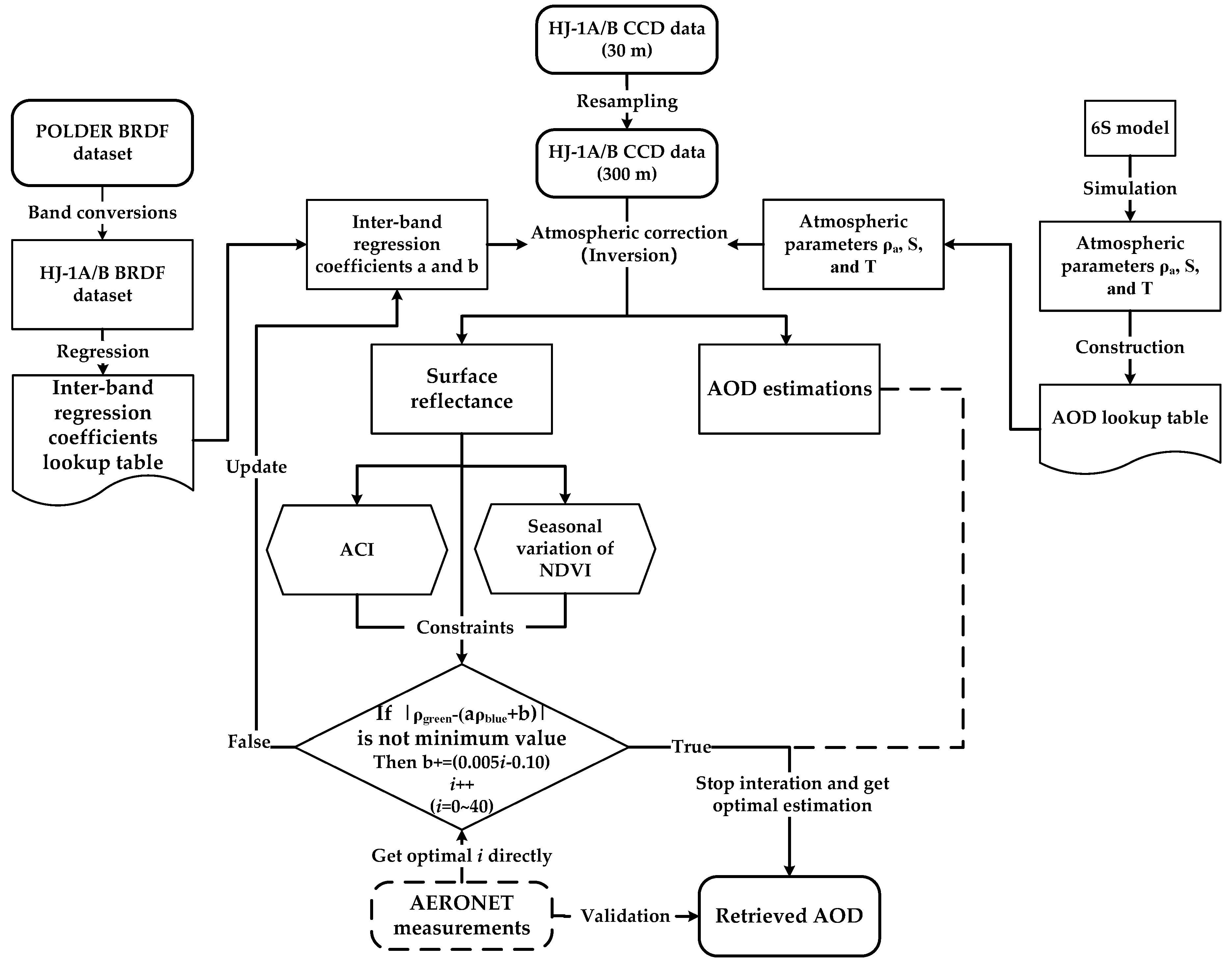
2.2. Overall Framework of the AOD Retrieval Algorithm

By assuming that a significant correlation exists between the visible bands, AOD could be retrieved based on the model simulated aerosol lookup table. However, this correlation varies with the solar/view angle and land cover type, so it was necessary to establish an interband regression coefficient lookup table based on the Bidirectional Reflectance Distribution Function (BRDF) dataset.

In this study, we first determined the correlation between the visible bands based on the U.S. Geological Survey (USGS) spectral library and selected the optical bands with the highest correlation to establish a linear regression relationship. Then, the POLarization and Directionality of the Earth’s Reflectances (POLDER) BRDF dataset was used to obtain the regression coefficients for different solar/view angles and land cover types. Finally, high-spatial resolution AODs could be retrieved based on a model simulated aerosol lookup table. In this procedure, the original HJ-1 A/B CCD data with a spatial resolution of 30 m were resampled to 300 m to minimize the effects of sensor noises. Because the inversion results were sensitive to the regression coefficients, an aerosol correction index (ACI), a seasonal variation of normalized differential vegetation index (NDVI), and AERONET measurements were employed as constraints to obtain optimal estimation. The flowchart of our method is shown in Figure 1.

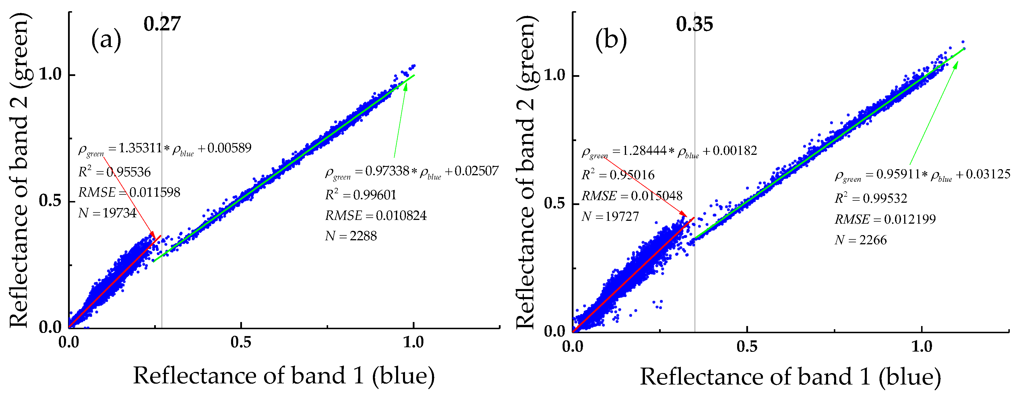
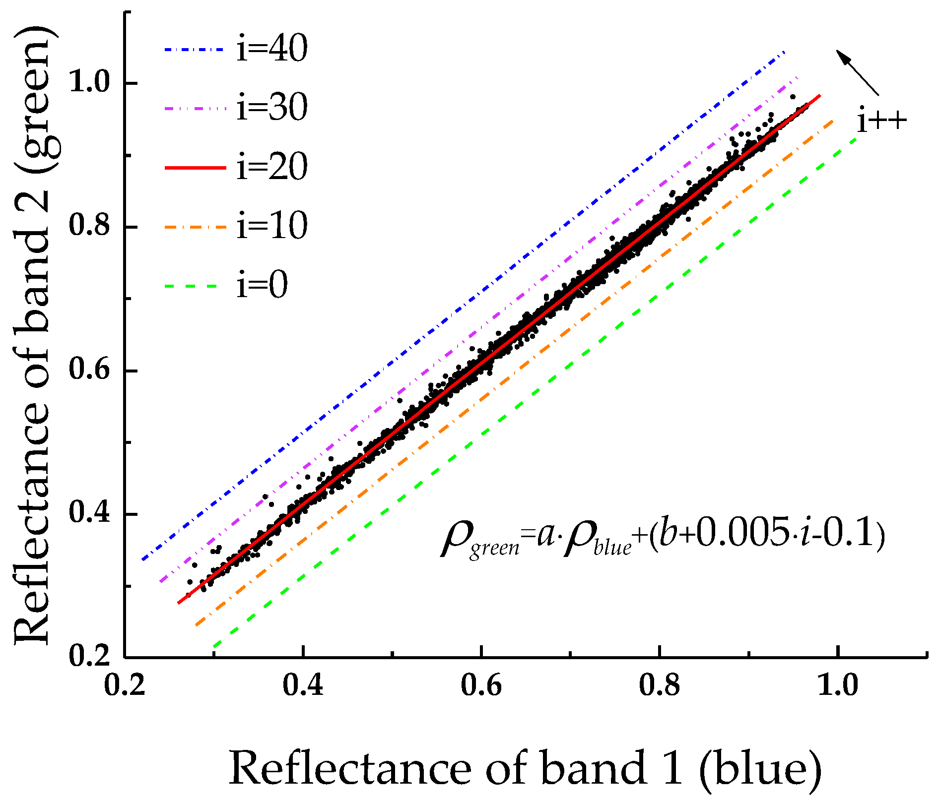
2.3. Interband Regression Coefficient Lookup Table

Based on a statistical analysis of the USGS spectral library, the visible bands of the HJ-1 A/B CCD data were well correlated. A linear regression relationship between the blue and green bands was established, as shown in Equation (1):

$${\rho }_{\mathrm{g}reen}=a\left({\theta }_s,{\theta }_v,\phi ;\omega \right)\cdot {\rho }_{blue}+b\left({\theta }_s,{\theta }_v,\phi ;\omega \right)$$

(1)

where ${\rho }_{blue}$ and ${\rho }_{green}$ are the reflectance of the blue and green bands (band 1 and 2 of HJ-1 A/B CCD data); and a and b denote the slope and intercept of the regression coefficients that vary with solar/view angle and land cover type ($\omega$), respectively.

To evaluate the applicability of the regression coefficients for different solar/view angles and land cover types, we analyzed the difference between the true and predicted value by the regression model:

$$Diff={\rho }_{green}-\left(a\left({\theta }_s,{\theta }_v,\phi ;\omega \right)\cdot {\rho }_{blue}+b\left({\theta }_s,{\theta }_v,\phi ;\omega \right)\right)$$

(2)

where $Diff$ is the difference between the true and predicted value, which can be used for evaluating the variations in interband regression coefficients from the solar/view angle and land cover type.

To determine the influence of solar/view angle and land cover type on the regression coefficient, we used the POLDER 3 BRDF dataset for analysis. The POLDER BRDF dataset is the latest multiangular satellite remote sensing data currently available. Featuring rich information in angle, spectrum, and polarization, it is one of the ideal datasets for evaluating land surface anisotropy effects. The POLDER sensor is able to collect observations from up to 16 viewing angles for each orbit, with a maximum view zenith angle of 60°. Hence, a monthly composite dataset can contain hundreds of observations from multiple orbits and viewing angles. The surface reflectance observed during all of the orbits was obtained through processing steps such as cloud removal and atmospheric correction [20]. The POLDER BRDF data files are in ASCII format, which provides the latitude and longitude of the pixels, land cover type (the global land cover of the year 2000, coordinated by the European Commission’s Joint Research Center), orbit number, effective times of observation (16 observations at most for each orbit), and the homogeneity of the pixel [21,22].

The HJ-1A/B BRDF dataset can be obtained from the POLDER BRDF dataset by a band conversion method. The band conversions from POLDER to HJ-1 A/B CCD can be expressed as

$${\rho }_{HJ}({\lambda }_i)={\displaystyle \sum _{i=1}^n{c}_i{\rho }_{POLDER}({\lambda }_i)+offset},$$

(3)

where ${\rho }_{HJ}({\lambda }_i)$ is the reflectance of the HJ-1 A/B CCD at a wavelength of ${\lambda }_i$, ${\rho }_{POLDER}({\lambda }_i)$ is the reflectance of POLDER-3 at a wavelength of ${\lambda }_i$, $c_i$ stands for the conversion coefficients for band $i$, and $offset$ stands for the offset coefficient (the conversion coefficients were provided by Sun et al. [23] (

Table 2. Band conversion coefficients from Polarization and Directionality of the Earth’s Reflectances (POLDER) to HJ-1 A/B CCD. BRDF: Bidirectional Reflectance Distribution Function; RMSE: Root mean square error.

Band	POLDER BRDF						Offset	RMSE
	C1	C2	C3	C4	C5	C6
HJ-Band1	0.777	0.212	−0.011	0.016	0.030	−0.028	−0.006	0.003
HJ-Band2	0.196	0.532	0.243	0.066	−0.010	−0.032	0.001	0.003
HJ-Band3	0.004	0.269	0.740	−0.050	−0.009	0.052	0.004	0.003
HJ-Band4	0.023	−0.008	−0.025	0.426	0.537	0.052	0.001	0.002

)).

Then, the blue and green bands of the HJ-1A/B CCD sensor were linearly regressed for different solar/view angles so as to establish an interband regression coefficient lookup table. In this lookup table, the solar zenith angle of 0–70° was separated into different angular bins with an interval of 2°, the view zenith angle of 0–40° was separated into angular bins with an interval of 2°, and the relative azimuth angle was separated into angular bins with an interval of 5°. The regression coefficients (a and b) for different solar/view angles were stored in a three-dimensional (solar zenith angle, view zenith angle, and relative azimuth angle) lookup table.

In addition, it is noted that in the interband regression procedure, a significant discontinuity point exists between the higher and lower reflectance (Figure 2a), and this discontinuity point changes with variation in the solar zenith angle. At the hotspot, the discontinuity point peaks, i.e., 0.35 (Figure 2b), whereas the value is relatively small (0.27) at other angles (Figure 2b). Compared to a global linear regression, the fitting accuracy can be much improved by splitting the datasets into two parts at the discontinuity point. In this study, the discontinuity points for different solar/view geometries were detected, and two regression procedures were performed for higher and lower reflectance datasets.

2.4. Aerosol Lookup Table

For retrieving the AOD from HJ-1 A/B CCD data, a model simulated aerosol lookup table was established in this study. We first assumed the surface and the atmosphere to be uniform and Lambertian. Then, the apparent reflectance ${\rho }^{*}$ received by the sensor of the satellite can be expressed as follows [24]:

$${\rho }^{*}({\theta }_s,{\theta }_v,\phi )={\rho }_a({\theta }_s,{\theta }_v,\phi )+\frac{{\rho }_s}{1-{\rho }_{s}S}T({\theta }_s)T({\theta }_v),$$

(4)

where ${\theta }_s$ and ${\theta }_v$ denote the solar and view zenith angle, respectively; $\phi$ denotes the solar and view azimuth angle; ${\rho }_a$ is the atmospheric path reflectance (the reflected contribution of the atmosphere); ${\rho }_s$ is the surface reflectance; $S$ is the atmospheric downward reflectance; and $T({\theta }_s)$ and $T({\theta }_v)$ are the downward and upward atmospheric transmittance, respectively.

Let $T=T({\theta }_s)T({\theta }_v)$, Equation (4), be simplified as

$${\rho }^{*}={\rho }_a+\frac{{\rho }_{s}T}{1-{\rho }_{s}S}.$$

(5)

Suppose there were three real values of surface reflectance (0.0, 0.5, and 0.8). Three corresponding apparent reflectances (${\rho }_1^{*}$, ${\rho }_2^{*}$, and ${\rho }_3^{*}$) can be obtained by the second simulation of the satellite signal in the solar spectrum model (the 6S model). According to Equation (5), the apparent reflectances ${\rho }_1^{*}$, ${\rho }_2^{*}$, and ${\rho }_3^{*}$ can also be expressed as

$${\rho }_1^{*}={\rho }_a+\frac{0.0T}{1-0.0S}={\rho }_a,$$

(6)

$${\rho }_2^{*}={\rho }_a+\frac{0.5T}{1-0.5S},$$

(7)

$${\rho }_3^{*}={\rho }_a+\frac{0.8T}{1-0.8S}.$$

(8)

By solving the simultaneous Equations (6)–(8), ${\rho }_a$, $T$, and $S$ can be derived as

$${\rho }_a={\rho }_1^{*},$$

(9)

$$T=2({\rho }_2^{*}-{\rho }_1^{*})(1-0.5S),$$

(10)

$$S=\frac{0.8{\rho }_2^{*}-0.5{\rho }_3^{*}-0.3{\rho }_1^{*}}{0.4({\rho }_2^{*}-{\rho }_3^{*})}.$$

(11)

Considering the computational accuracy and efficiency of the computer, the solar zenith, view zenith, and relative azimuth angles were divided at 6°, 3°, and 12° as the intervals, respectively. The 6S model [24] was used to repeat the above process to simulate ${\rho }_a$, $S$, and $T$, corresponding to different solar/view angles and AOD conditions (with an interval of 0.05), and a four-dimensional (solar zenith angle, view zenith angle, relative azimuth angle, and AOD) aerosol lookup table was established.

Table 3. Input parameters of 6S model.

Variables	Input Parameters
Solar zenith angle	0°, 6°, 12°, 18°, 24°, 30°, 36°, 42°, 48°, 54°, 60°, 66°
View zenith angle	0°, 3°, 6°, 9°, 12°, 15°, 18°, 21°, 24°, 27°, 30°, 33°, 36°, 39°
Relative azimuth angle	0°, 12°, 24°, 36°, 48°, 60°, 72°, 84°, 96°, 108°, 120°, 132°, 144°, 156°, 168°, 180°
Atmospheric model	Mid-latitude summer
Aerosol Type	Continental
AOD	0.0001, 0.05, 0.1, 0.15, 0.2, 0.25, 0.3, 0.35, 0.4, 0.45, 0.5, 0.55, 0.6, 0.65, 0.7, 0.75, 0.8, 0.85, 0.9, 0.95, 1.0, 1.05, 1.1, 1.15, 1.2, 1.25, 1.3, 1.35, 1.4, 1.45, 1.5, 1.55, 1.6, 1.65, 1.7, 1.75, 1.8, 1.85, 1.9, 1.95

shows the input parameters for the 6S model (in this study, we took a mid-latitude summer atmosphere and continental aerosol type as an example).

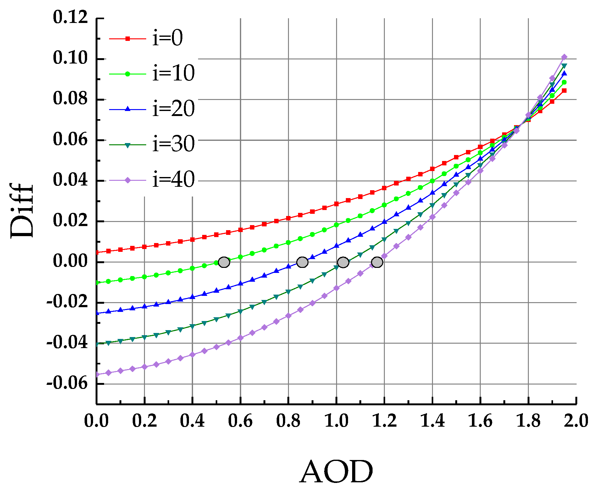
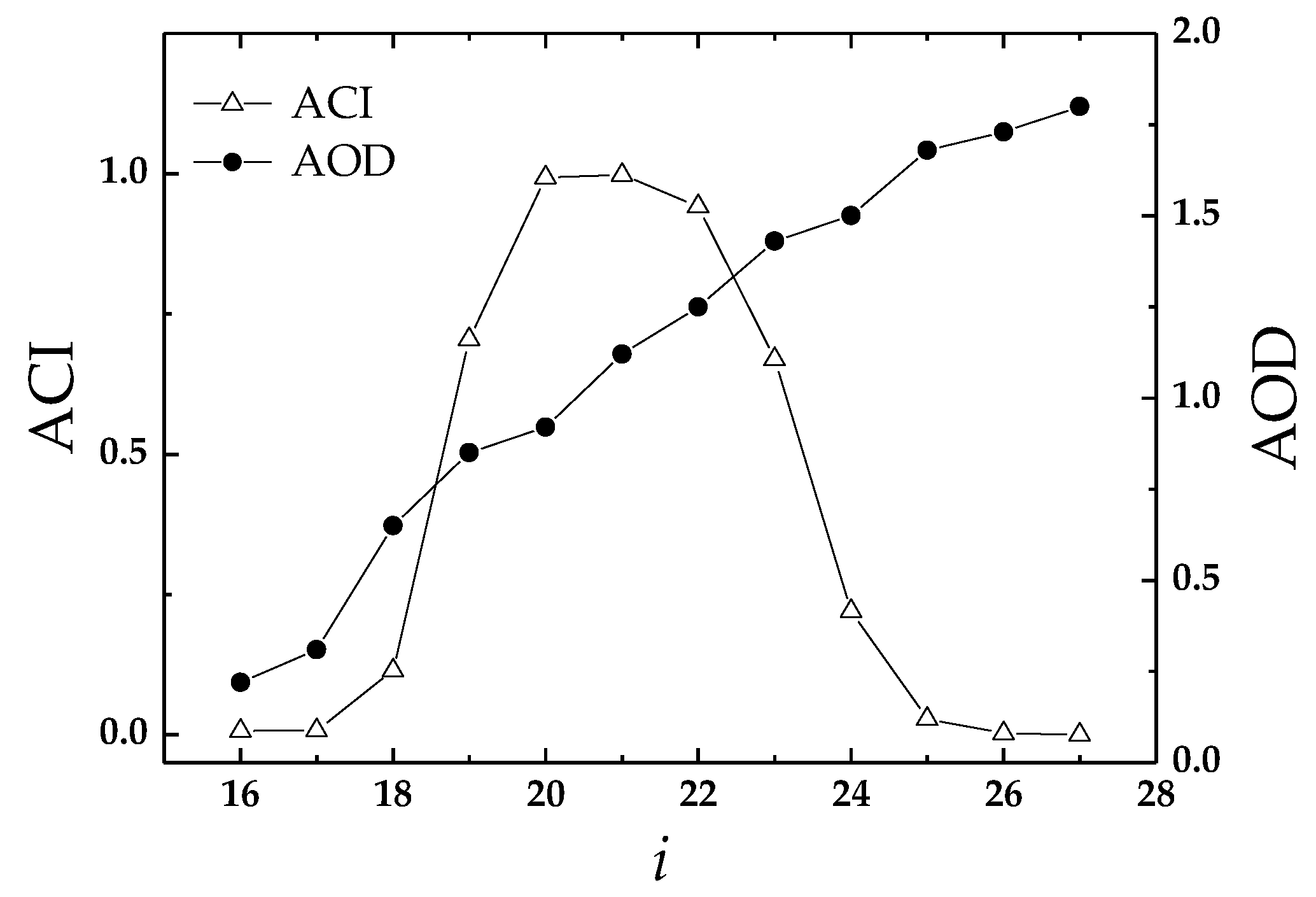
2.5. Retrieval of AOD with Constraints

Based on the interband regression coefficients and the aerosol lookup table, AOD can be retrieved from the apparent reflectance of the HJ-1 A/B CCD. For a specific pixel, the atmospheric parameters ${\rho }_a$, $T$, and $S$ at a prescribed solar/view geometry and different AOD conditions can be obtained from the aerosol lookup table. Thus, atmospheric correction procedures were performed assuming the AOD level. The optimal AOD estimation can be obtained by searching the minimum value of the following object function:

$$\delta =\left|{\stackrel{⌢}{\rho }}_{green}(\tau )-(a{\stackrel{⌢}{\rho }}_{blue}(\tau )+b)\right|,$$

(12)

where $\delta$ stands for the object function, and ${\widehat{\rho }}_{green}(\tau )$ and ${\widehat{\rho }}_{blue}(\tau )$ are the atmospheric-corrected reflectance of green and blue bands for an assumed AOD level $\tau$, respectively. The interband regression coefficients (a and b) can be obtained by the lookup table of regression coefficients.

However, we found it difficult to get the optimal AOD estimation due to the systematic errors of the imageries, such as calibration issues with the HJ-1 A/B CCD data. Since the regression intercept b was not robust due to the systematic error, a correction for the intercept b was requested by this study. The results of the sensitivity analysis showed that a change of 0.05 in the regression intercept (b) could lead to a change of about 0.2–0.3 in the retrieved AOD (Figure 3). Therefore, an offset step i for an entire image was added to each regression intercept b (with 0.005 as the interval, bi = b + (i × 0.005 − 0.10), i = 0~41) (Figure 4).

The above-mentioned object function can be adopted as follows:

$$\delta =\left|{\stackrel{⌢}{\rho }}_{green}(\tau )-(a{\stackrel{⌢}{\rho }}_{blue}(\tau )+b+i\times 0.005-0.10)\right|.$$

(13)

There are two approaches for determining the offset step i: (1) If the AOD measurements can be used as prior knowledge, the offset step i for an entire image can be determined directly by Equation (13); (2) if there are no available AOD measurements, optimal estimations of AOD and offset step (i) can be retrieved with the constraints of the ACI and seasonal variations of the NDVI. With this approach, the ACI was first used for narrowing the searching range of i, and then the seasonal variations of the NDVI were used as references for getting the optimal AOD estimations.

The ACI is defined as the normalized difference of atmospheric-corrected reflectance of near-infrared and blue bands:

$$ACI=\frac{{\widehat{\rho }}_{NIR}-\left|{\widehat{\rho }}_{blue}\right|}{{\widehat{\rho }}_{NIR}+\left|{\widehat{\rho }}_{blue}\right|},$$

(14)

where ${\widehat{\rho }}_{NIR}$ and ${\widehat{\rho }}_{blue}$ are the atmospheric-corrected reflectance of near-infrared (NIR) and blue bands with different offset steps i, respectively.

In this study, the ACI was used to narrow the search range of i and avoid the occurrence of excessive atmospheric correction. As the offset step i increases, the intercept b and the retrieved AOD also increase, and excessive atmospheric correction occurs. When excessive atmospheric correction occurs, the blue band decreases to a negative value, whereas the AOD exerts a small influence on the near-infrared band. Therefore, it can be approximately deemed that the near-infrared band does not change with atmospheric correction, and the ACI curve shows a trend of initially increasing and then decreasing (Figure 5). The values of the offset steps that indicated that excessive atmospheric correction occurred were screened out.

The seasonal variation of the NDVI was used as a constraint to further determine AOD estimation. The NDVI was first calculated with atmospheric-corrected reflectance over a dense vegetation-covered area. Then, the temporal variation of the NDVI was fitted with a quadratic function (Figure 6). The optimal offset step i can be obtained when the objection function ${\delta }_{NDVI}$ reaches the minimum value

$${\delta }_{NDVI}=\left|NDVI(i,t)-N\tilde{D}VI(t)\right|$$

(15)

where $NDVI(i,t)$ is the zonal mean NDVI with an offset step i at time t; and $N\tilde{D}VI(t)$ is the fitting result of the NDVI at time t. It is noted that this constraint is only useful during the growing [25] season of vegetation and is not applicable in winter.

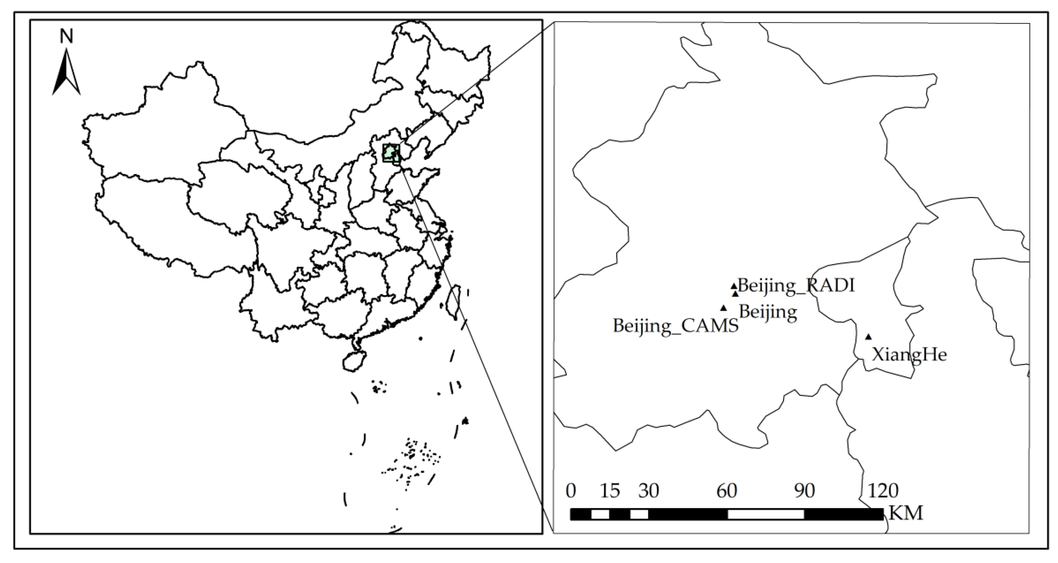
2.6. Data and Method for Validation

In this study, a validation of AOD estimations was carried out with the surface measurement data from four sites of the Aerosol Robotic Network (AERONET) in Beijing. Figure 7 shows the geolocations of these four sites (the latitudes and longitudes are shown in

Table 4. Summary of AERONET sites.

Site	Longitude (Degree)	Latitude (Degree)	Approach I	Approach II
			The Years Used for Validation	The Years Used As an Input	The Years Used for Validation
Beijing	116.381	39.977	2013–2015	2014	2012, 2013, 2015
Beijing_CAMS	116.317	39.933	2013–2015	2012, 2015	2013, 2014
Beijing_RADI	116.379	40.005	2013–2015	—	2012, 2013, 2014, 2015
XiangHe	116.962	39.754	2013–2015	2013	2012, 2014, 2015

). As a federation of ground-based aerosol measurement networks (https://aeronet.gsfc.nasa.gov/), AERONET uses CE-318 automatic solar photometers to measure direct and scattered radiation from the sun. These photometers provide near-real-time observational data, such as globally distributed aerosol spectral optical depth and aerosol particle size distribution [26], which can retrieve optical parameters such as single scattering albedo, asymmetry factors, and scattering phase functions of aerosol particles [27]. Less influenced by surface parameters and aerosol forward scatter [28], these photometers have an AOD acquisition accuracy of 0.02–0.01 [29] and are widely used in verifying AOD estimations. The data can be divided into the unscreened Level 1.0 product, the cloud-detected Level 1.5 product, and the Level 2.0 product, which has undergone cloud detection and quality control.

In this study, the AOD retrieved from satellite observations was the AOD at 550 nm. However, the AERONET does not contain observations at this wavelength, and interpolation needed to be conducted [25]:

$$\tau (\lambda )=\beta \cdot {\lambda }^{\alpha },$$

(16)

where $\tau$ is the AOD at wavelength $\lambda$, $\alpha$ is the Ångstrӧm index, and $\beta$ is the atmospheric turbidity coefficient.

Four statistical indicators, namely root mean square error (RMSE), mean absolute error (MAE), and expected error (EE), were used to validate and analyze the inversion results. Meanwhile, EE represents the percentage of retrieved results within the envelope of the expected error region, defined as

$$\Delta \tau ={\tau }_i\pm (0.05+0.20{\tau }_i),$$

(17)

where $\Delta \tau$ is the envelope of the expected error region (error lines), and ${\tau }_i$ is the AOD measured by the AREONET sites.

In this study, two approaches were carried out for validation of the AODs retrieved from HJ-1 A/B CCD data. In validation approach I, in situ measurements of four AERONET sites were all used for validation. In validation approach Ⅱ, the simplified aerosol retrieval algorithm (SARA) approach [30,31,32] was adopted to improve the quality of the retrievals. In this approach, parts of the AERONET measurement data were used as an input for obtaining an optimal offset step i, and the other measurements were used for validation. In the year 2012, the Beijing_CAMS site was used as an input, and the Beijing, Beijing_RADI, and XiangHe sites were used for validation; in the year 2013, the XiangHe site was used as an input, and the Beijing, Beijing_RADI, and Beijing_CAMS sites were used for validation; in the year 2014, the Beijing site was used as an input, and the XiangHe, Beijing_RADI, and Beijing_CAMS sites were used for validation; and in the year 2015, the Beijing_CAMS site was used as an input, and the Beijing, Beijing_RADI, and XiangHe sites were used for validation.

3. Results and Discussion

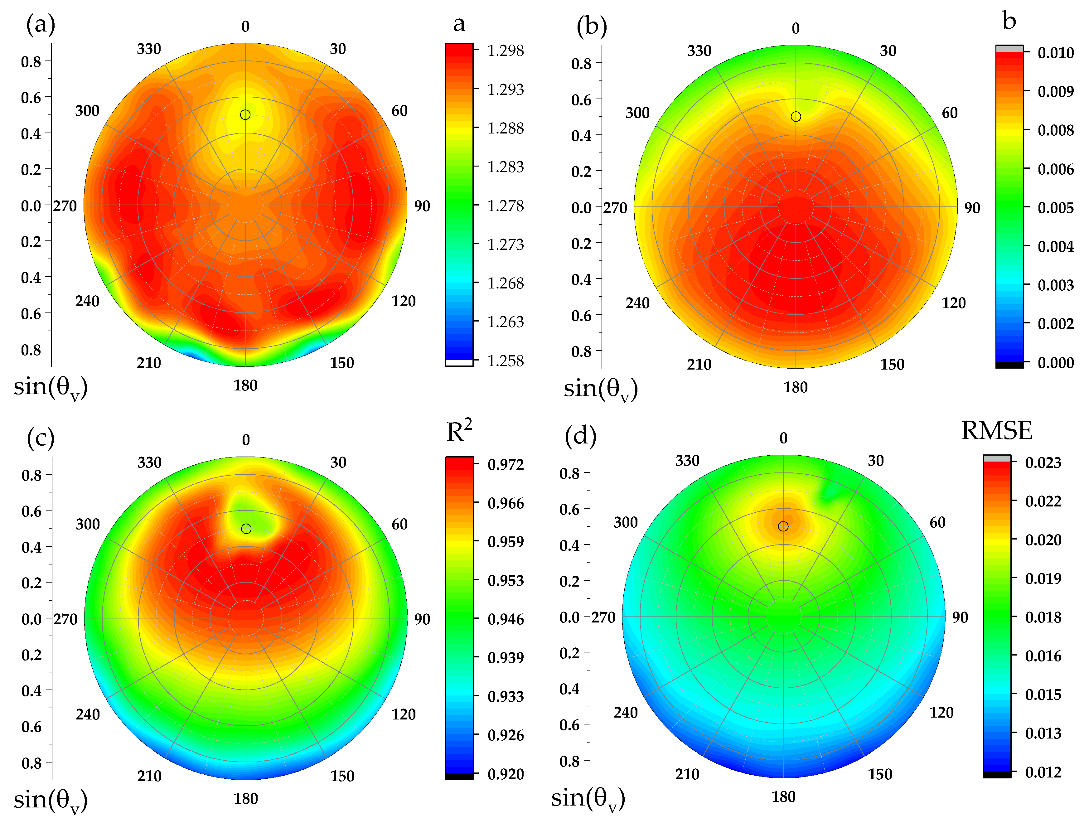
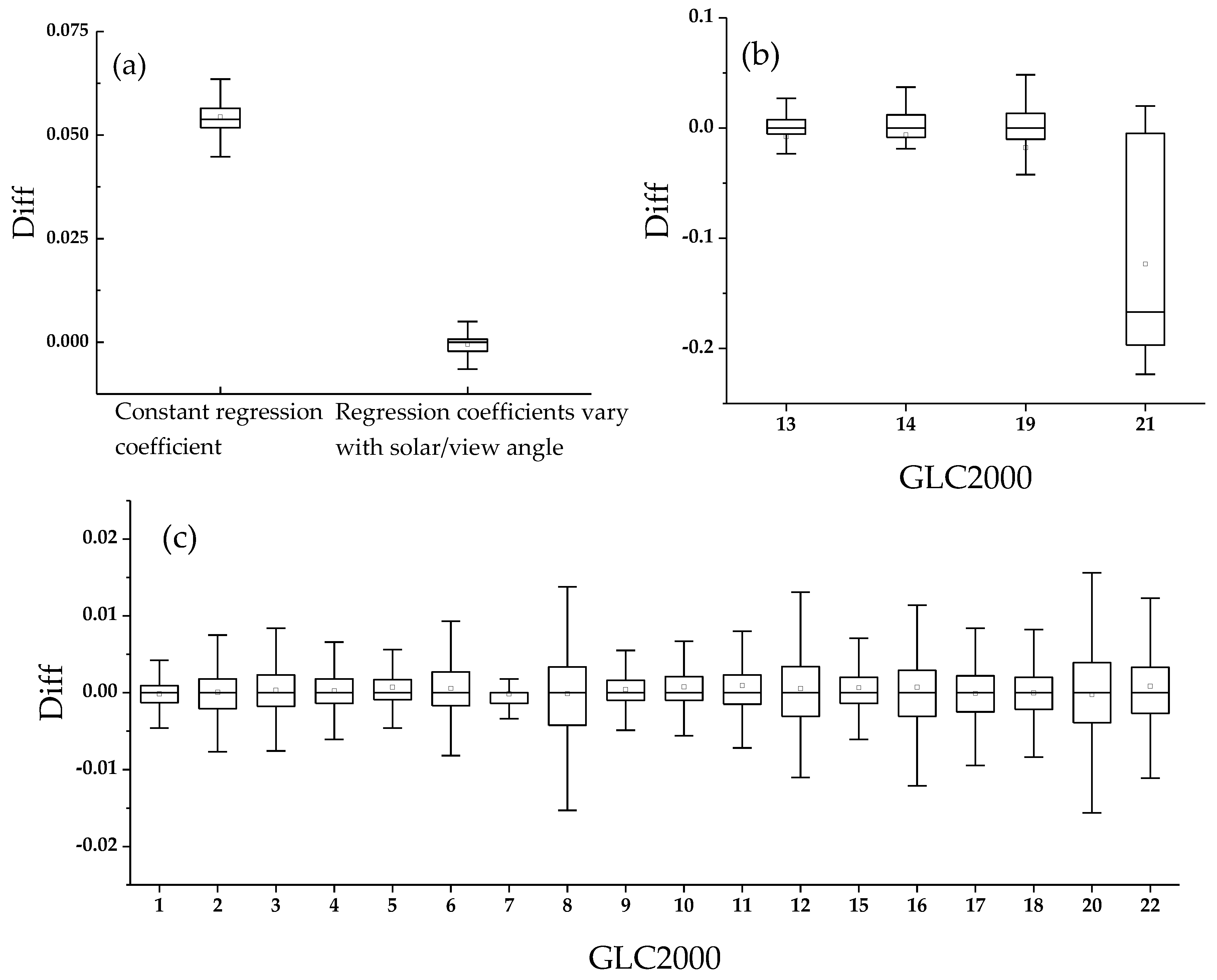
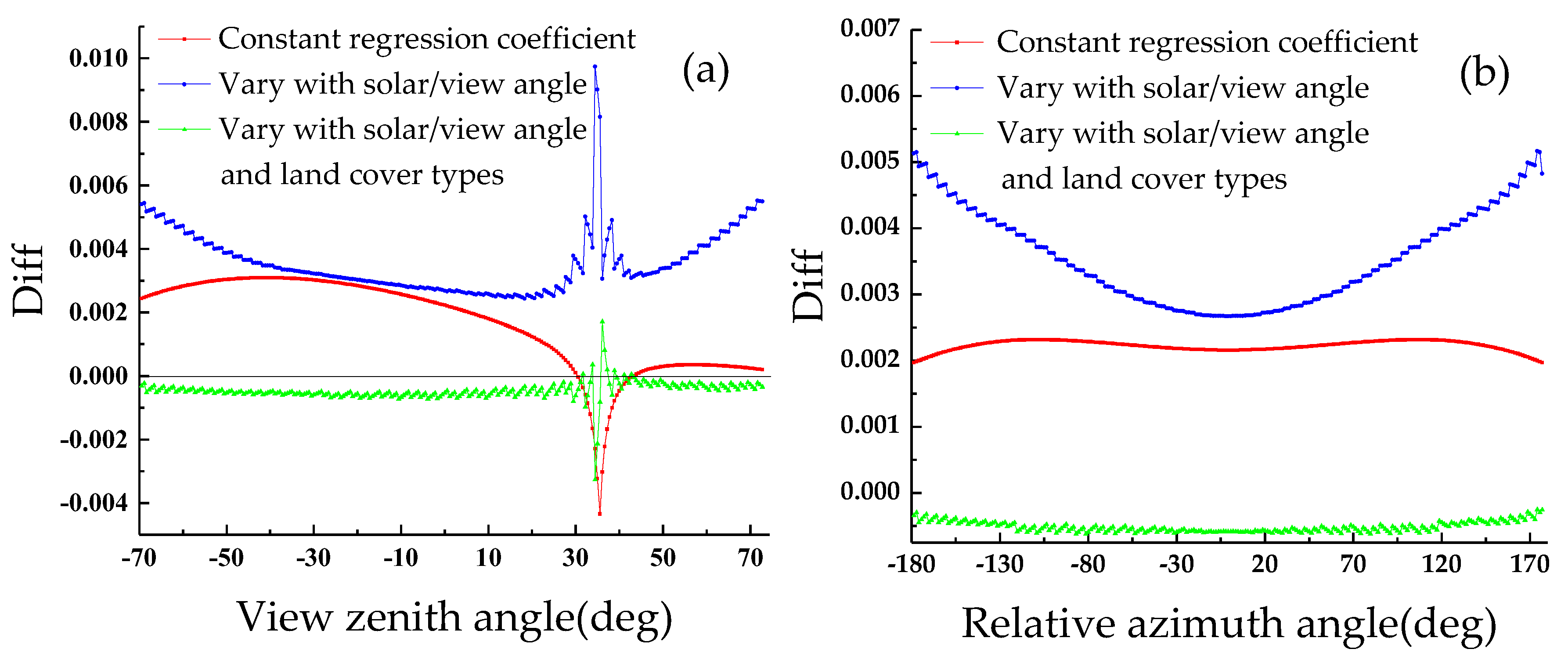
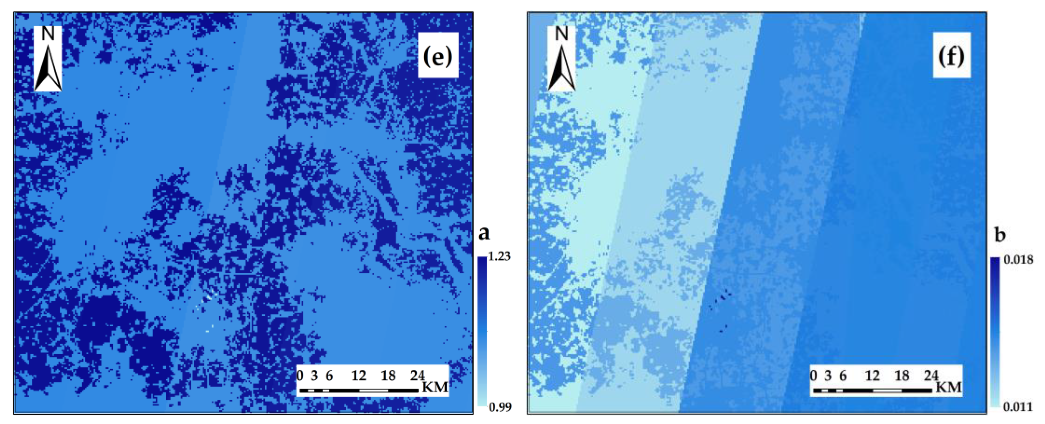
3.1. Sensitivity Analysis of Interband Regression Coefficients

To evaluate the sensitivity of the interband regression coefficients, four scenarios were carried out for comparison in this study: (1) A constant regression coefficient that did not vary by solar/view angle and land cover type; (2) regression coefficients that varied with different solar/view angles; (3) regression coefficients that varied with different land cover types; (4) and regression coefficients that varied with different solar/view geometries and land cover types. In the case of using a constant regression coefficient (Figure 8a), the overall offset error was 0.05, and the difference between the maximum and minimum values over the semi-hemispherical space was about 0.013. In contrast, in the case of using regression coefficients varying with the solar/view angle, the difference between the maximum and minimum values was about 0.014 (Figure 8a). In the case of using regression coefficients varying by land cover type, the overall dispersion was smaller for most of the land cover types, with a standard deviation of 0.0048, and there was a difference between the maximum and minimum values over the semi-hemispherical space of about 0.015 (Figure 8c). However, grasslands, shrubs, and bare land, as well as snow and ice (corresponding to GLC2000 land cover types 13, 14, 19, and 21) had relatively large errors (Figure 8b). In the case of using regression coefficients varying by solar/view geometry and land cover type, the values of Diff were around 0, with a mean of −0.00004 and a standard deviation of 0.0031 (Figure 9). It can be seen that in the principal and the perpendicular planes, the influence of solar/view angle on the interband regression coefficients could be better corrected by using regression coefficients varying with different solar/view angles and land cover types.

Significant variations existed in the values of interband regression coefficients a and b over the semi-hemispherical space, especially at the hotspot and at the large view zenith angles (Figure 10). The fitted R² was relatively small and the RMSE was relatively large at the hotspot and large view zenith angles, with an overall R² exceeding 0.91 and an overall RMSE below 0.023, indicating that the interband regression coefficients a and b had a good overall fitting effect for the HJ-1 A/B CCD data (with a maximum view zenith angle of 35°).

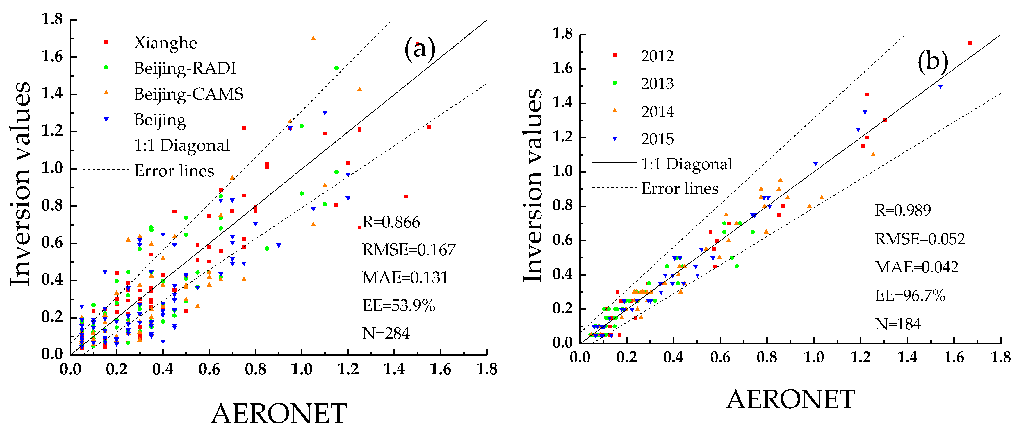
3.2. Validation with AERONET Measurements

Images observed by the HJ-1 A/B satellite from April to October during 2012–2015 were used in this study. The Level 2.0 product of AERONET measurements within 1.5 h of satellite overpass time were employed for validation. The AOD retrieved from the HJ-1 A/B CCD data was compared with in situ-measured AOD data at the XiangHe, Beijing-RADI, Beijing-CAMS, and Beijing sites (Table 4). Figure 11a shows a scatter plot of AODs retrieved without any prior knowledge versus AERONET measurements (validation approach Ⅰ). It can be seen that the overall correlation coefficient R was 0.866, the RMSE was 0.167, and the MAE was 0.131, and EE reached 53.9%. The correlation coefficients of the four sites were all above 0.8, with that of the XiangHe site reaching above 0.9. The inversion accuracy of the vegetated areas (XiangHe) was slightly higher than that of the urban areas (Beijing-RADI, Beijing-CAMS, and Beijing). Therefore, the R and EE of the XiangHe site were greater than those of the other three sites, whereas its RMSE and MAE were smaller than those of the other three sites. As can be seen from the scatter plot, the inversion results were distributed around the 1:1 diagonal, with a relatively large error when AOD was low. If the AOD measurements of an AERONET site were used as prior knowledge to get optimal offset step i, and the measurements of other AERONET sites were used for validation (validation approach Ⅱ), the AOD of the entire image could be much more accurately obtained by this method (R is 0.989, RMSE is 0.052, MAE is 0.042, and EE is 96.7%; Figure 11b).

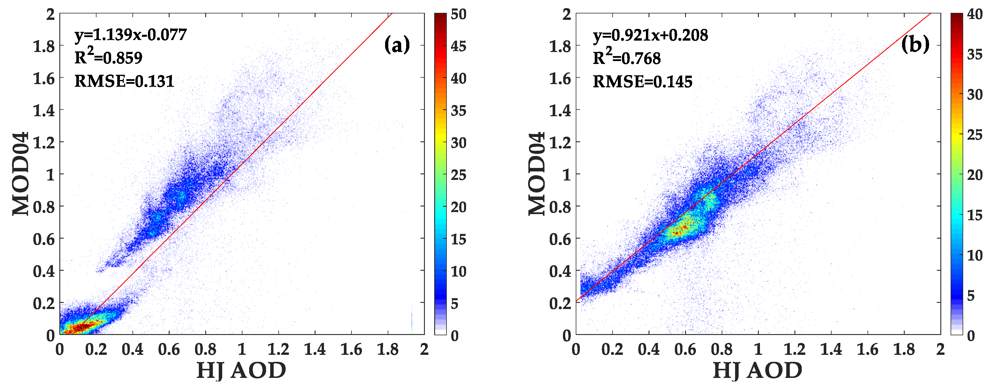
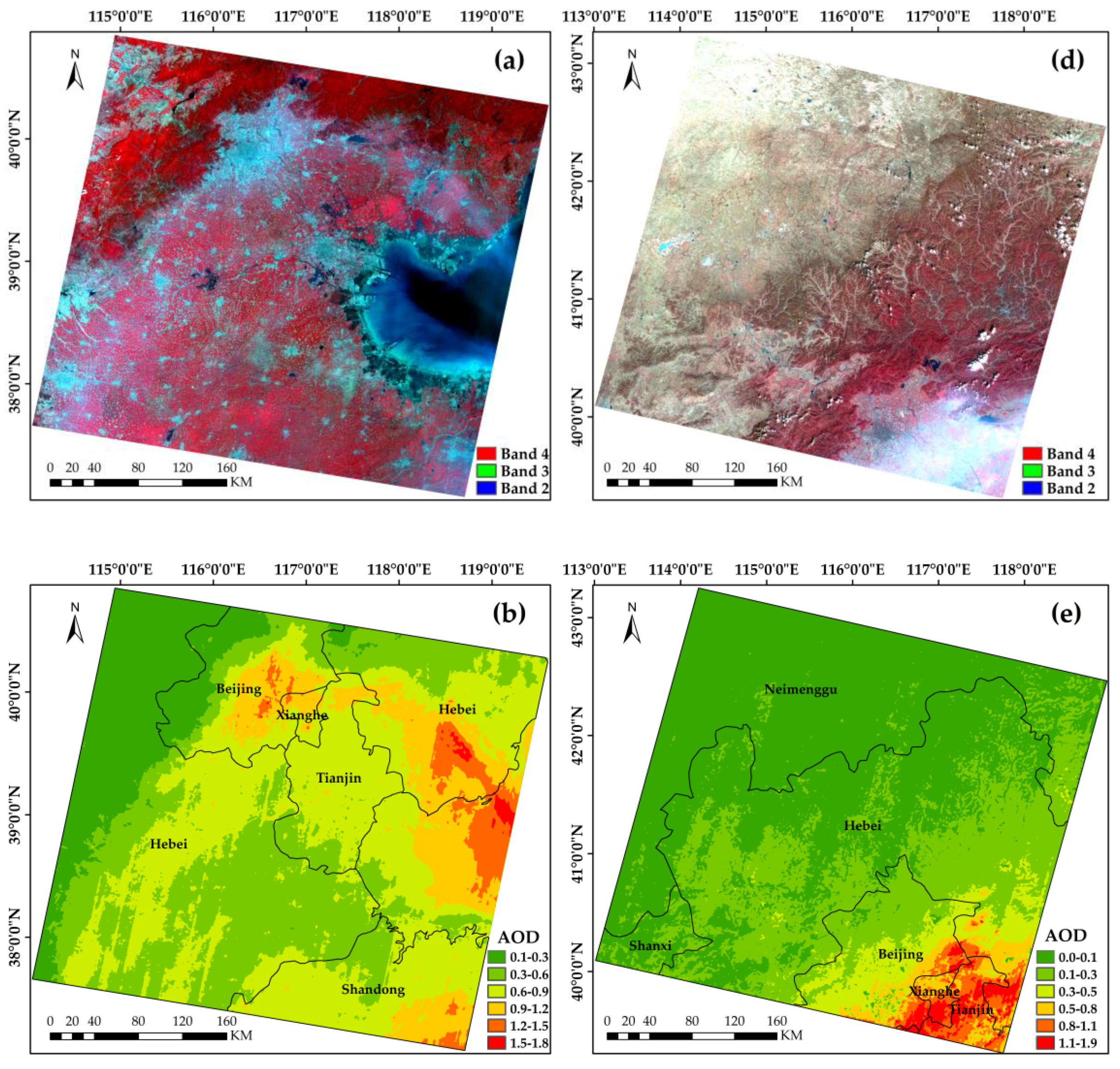
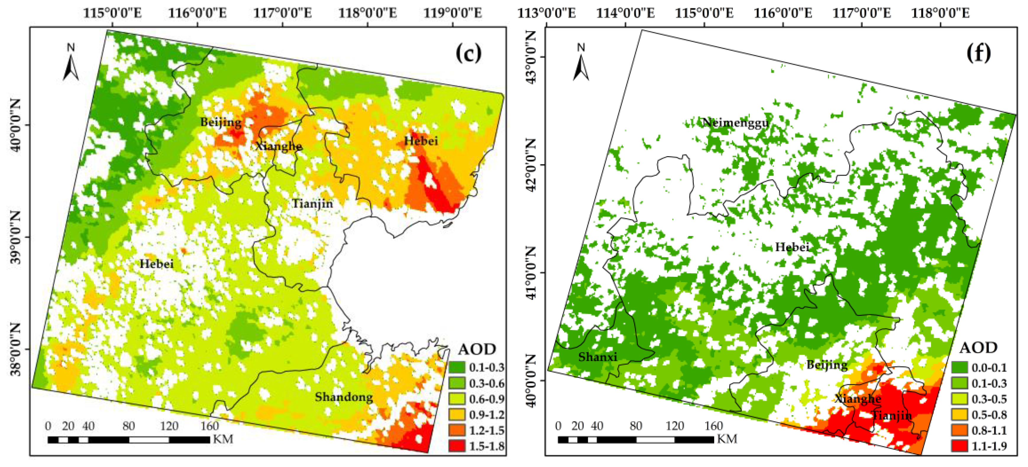
3.3. Comparison with MODIS Aerosol Product

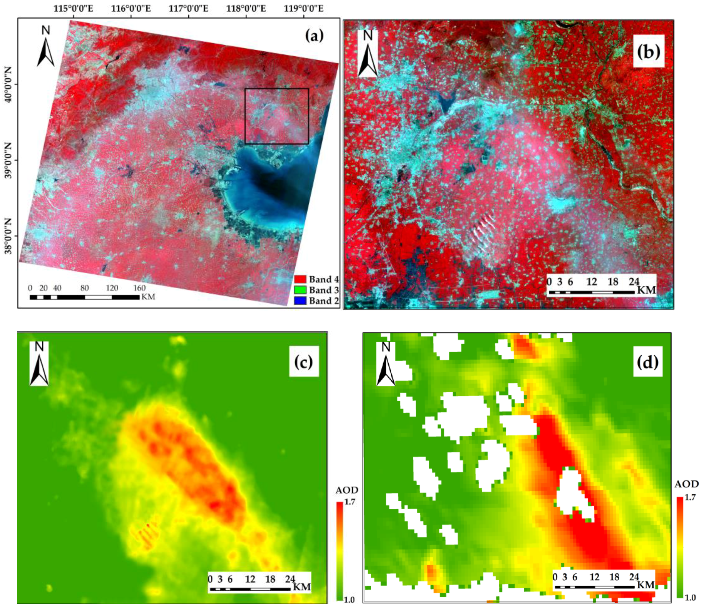
The MODIS aerosol product (MOD04_3K) with a spatial resolution of 3 km was employed for comparison to the AODs retrieved from the HJ-1 A/B CCD data. Figure 12a,d shows the false color HJ-1 A/B CCD images (band 4 is displayed in a red color, band 3 is displayed in a green color, and band 2 is displayed in a blue color) observed on 26 July 2014 and 6 October 2012, respectively. Figure 12b,e shows the AOD dataset retrieved from the HJ-1 A/B CCD data, whereas Figure 12c,f shows the corresponding MODIS aerosol products with an overpass time within 1.5 h. The comparison results showed that the AOD retrieved from the HJ-1 A/B CCD data agreed well with the distribution range and trend of the visual interpretation and the MODIS aerosol product. From Figure 12c,f, a serious data-missing phenomenon can be observed in the MODIS aerosol product. In contrast, the AOD retrieved by the algorithm proposed in this study can avoid such a situation. Figure 13 shows the partially enlarged image of Figure 12a (upper-right corner) and the corresponding AOD map retrieved from the HJ-1 A/B CCD data and the MODIS aerosol product. From these figures, it can be seen that the AOD maps retrieved from the HJ-1 A/B CCD data had a high spatial resolution, making a remarkable improvement when compared to the image quality of the MODIS aerosol product. The comparison results with the MODIS aerosol product showed that the AOD map retrieved from HJ-1 A/B showed superior image quality to that of the MODIS aerosol product. The density plots of the AOD retrieved from the HJ-1 A/B CCD data versus the MODIS aerosol products are shown in Figure 14. The results showed that the AOD estimation results of the MODIS aerosol product were lower than the AODs retrieved from the HJ-1 A/B CCD data for a relatively low AOD case, with an R² of 0.859 and an RMSE of 0.131 (Figure 14a). The estimation results of the MODIS aerosol product were 0.208 higher than the AODs retrieved from the HJ-1 A/B CCD data (Figure 14b) for a high AOD case, with an R² of 0.768 and an RMSE of 0.145.

3.4. Discussion

The comparison and validation results showed that the method proposed by this study could improve the image quality AOD estimations and provide an alternate method for retrieving AODs from remote sensing data without SWIR bands, such as HJ-1 A/B CCD data. The main issues and research prospects of this method are summarized as follows:

(1) AOD retrieval accuracy could be significantly improved once the measurements of an AERONET site were used as prior knowledge [30,31,32]. The main reason for this phenomenon was that the estimation of offset step i of the regression intercept could be seriously affected by issues of sensor calibration. Thus, in situ-measured AOD could be used as a calibration dataset for various satellite imageries, getting the optimal estimation of offset step i directly and improving the estimation accuracy of AODs derived from satellite observations;

(2) In this study, to avoid the effects of sensor noises, the HJ-1 A/B CCD data were first resampled to 300 m, and then the AOD was retrieved from the low spatial resolution data. We have to admit that this processing procedure reduced the real spatial resolution of the retrieved AOD dataset. However, the image quality of HJ-1 A/B CCD AOD was still superior to that of the MODIS 3 km aerosol product;

(3) The results of the sensitivity analysis showed that the interband regression coefficients varied by solar/view angle and land cover type. If the interband regression coefficient was assumed as a constant or not well considered, a large estimation error could occur. Therefore, establishing an interband regression coefficient lookup table is critically important for accurately retrieving the AOD from satellite observations;

(4) The method proposed by this study can be applied to various remote sensing sensors and application scenarios. Once the sensor has visible and NIR bands, the AOD can be retrieval. It can be applied to commonly used satellite data, such as Landsat TM/ETM/ETM+, MODIS, POLDER, etc., and also has a great advantage in retrieving AODs from the sensors without SWIR bands, i.e., Quickbird CCD, Chinese Gaofen series satellite sensors, and low-cost cameras onboard unmanned aerial vehicles (UAVs).

4. Conclusions

In this study, an algorithm for retrieving high-spatial resolution AODs from HJ-1 A/B CCD data was proposed. The AOD was retrieved based on interband regression coefficients that varied by solar/view angle and land cover type and a model simulated aerosol lookup table. This algorithm provides a method for retrieving AODs from sensors without SWIR bands, which can be useful for various remote sensing sensors and application scenarios. The inversion results were validated with surface measurements and compared to the MODIS aerosol product. The results showed that the AODs retrieved by this method were superior to the MODIS aerosol product in terms of image quality. The validation results showed that the retrieved AODs were consistent with in situ measurements with an R of 0.866, RMSE of 0.167, MAE of 0.131, and EE of 53.9%. If the AOD of a specific point in the image was given, the AOD of the entire image could be much more accurately obtained by this method (R is 0.989, RMSE is 0.052, MAE is 0.042, and EE is 96.7%).

References

1. Qiu, J. A Method to Determine Atmospheric Aerosol Optical Depth Using Total Direct Solar Radiation. J. Atmos. Sci. 1998, 55, 744–757. [Google Scholar] [CrossRef]
2. Anderson, J.C.; Wang, J.; Zeng, J.; Petrenko, M.; Leptoukh, G.G.; Ichoku, C. Accuracy assessment of Aqua-MODIS aerosol optical depth over coastal regions: Importance of quality flag and sea surface wind speed. Atmos. Meas. Tech. Discuss. 2012, 2012, 5205–5243. [Google Scholar] [CrossRef]
3. King, M.D.; Kaufman, Y.J.; Tanré, D.; Nakajima, T. Remote Sensing of Tropospheric Aerosols from Space: Past, Present, and Future. Bull. Am. Meteorol. Soc. 1999, 80, 2229–2260. [Google Scholar] [CrossRef]
4. Kaufman, Y.J.; Gobron, N.; Pinty, B.; Widlowski, J.-L.; Verstraete, M.M. Relationship between surface reflectance in the visible and mid-IR used in MODIS aerosol algorithm—Theory. Geophys. Res. Lett. 2002, 29, 31-1–31-34. [Google Scholar] [CrossRef]
5. Sun, L.; Sun, C.; Liu, Q.; Zhong, B. Aerosol optical depth retrieval by HJ-1/CCD supported by MODIS surface reflectance data. Sci. China Earth Sci. 2010, 53, 74–80. [Google Scholar] [CrossRef]
6. Kaufman, Y.J.; Wald, A.E.; Remer, L.A.; Gao, B.C.; Li, R.R.; Flynn, L. The MODIS 2.1-/spl mu/m channel-correlation with visible reflectance for use in remote sensing of aerosol. IEEE Trans. Geosci. Remote Sens. 1997, 35, 1286–1298. [Google Scholar] [CrossRef]
7. Kaufman, Y.J.; Remer, L.A. Detection of forests using mid-IR reflectance: An application for aerosol studies. IEEE Trans. Geosci. Remote Sens. 1994, 32, 672–683. [Google Scholar] [CrossRef]
8. Levy, R.C.; Remer, L.A.; Mattoo, S.; Vermote, E.F.; Kaufman, Y.J. Second-generation operational algorithm: Retrieval of aerosol properties over land from inversion of Moderate Resolution Imaging Spectroradiometer spectral reflectance. J. Geophys. Res. Atmos. 2007, 112. [Google Scholar] [CrossRef]
9. Hsu, N.C.; Si-Chee, T.; King, M.D.; Herman, J.R. Aerosol properties over bright-reflecting source regions. IEEE Trans. Geosci. Remote Sens. 2004, 42, 557–569. [Google Scholar] [CrossRef]
10. Hsu, N.C.; Tsay, S.; King, M.D.; Herman, J.R. Deep Blue Retrievals of Asian Aerosol Properties During ACE-Asia. IEEE Trans. Geosci. Remote Sens. 2006, 44, 3180–3195. [Google Scholar] [CrossRef]
11. Tian, X.; Sun, L.; Liu, Q.; Li, X. Retrieval of high-resolution aerosol optical depth using Landsat 8 OLI data over Beijing. J. Remote Sens. 2018, 51–63. [Google Scholar] [CrossRef]
12. Wang, Z.T.; Li, Q.; Wang, Q.; Li, S.; Chen, L.; Zhou, C.Y.; Zhang, L.J.; Xu, Y.J. HJ-1 terrestrial aerosol data retrieval using deep blue algorithm. J. Remote Sens. 2012, 16, 596–610. [Google Scholar]
13. Remer, L.A.; Mattoo, S.; Levy, R.C.; Munchak, L.A. MODIS 3 km aerosol product: Algorithm and global perspective. Atmos. Meas. Tech. 2013, 6, 1829–1844. [Google Scholar] [CrossRef]
14. Wang, Z.; Li, Q.; Tao, J.; Li, S.; Wang, Q.; Chen, L. Monitoring of aerosol optical depth over land surface using CCD camera on HJ-1 satellite. China Environ. Sci. 2009, 29, 902–907. [Google Scholar]
15. Zhao, Z.; Li, A.; Bian, J.; Huang, C. An improved DDV method to retrieve AOT for HJ CCD image in typical mountainous areas. Spectrosc. Spectral Anal. 2015, 35, 1479–1487. [Google Scholar] [CrossRef]
16. Sun, L.; Liu, Q.; Chen, L.; Liu, Q. The Application of HJ-1 Hyper spectral Imaging Radiometer to Retrieve Aerosol Optical Thickness over Land. J. Remote Sens. 2006, 10, 770–776. [Google Scholar]
17. Wang, Z.; Wang, H.; Li, Q.; Zhao, S.; Li, S.; Chen, L. A quickly atmospheric correction method for HJ-1 CCD with deep blue algorithm. Spectrosc. Spectral Anal. 2014, 34, 729–734. [Google Scholar] [CrossRef]
18. Sun, L.; Wei, J.; Bilal, M.; Tian, X.; Jia, C.; Guo, Y.; Mi, X. Aerosol Optical Depth Retrieval over Bright Areas Using Landsat 8 OLI Images. Remote Sens. 2016, 8, 23. [Google Scholar] [CrossRef]
19. Li, S.; Chen, L.; Tao, J.; Han, D.; Wang, Z.; Su, L.; Fan, M.; Yu, C. Retrieval of aerosol optical depth over bright targets in the urban areas of North China during winter. Sci. China Earth Sci. 2012, 55, 1545–1553. [Google Scholar] [CrossRef]
20. Hautecœur, O.; Leroy, M.M. Surface bidirectional reflectance distribution function observed at global scale by POLDER/ADEOS. Geophys. Res. Lett. 1998, 25, 4197–4200. [Google Scholar] [CrossRef]
21. Alonso, L.; Moreno, J.; Leroy, M. BRDF Signatures from Polder Data. In The Digital Airborne Spectrometer Experiment (DAISEX), Proceedings of the Workshop Held July 2001; Wooding, M., Harris, R.A., Eds.; ESA SP-499; European Space Agency: Paris, France, 2001; p. 183. [Google Scholar]
22. POLDER-3/PARASOL BRDF Databases User Manual 2009. Available online: https://www.theia-land.fr/sites/default/files/imce/produits/polder-3_brdf_usermanual-i1.20-22_doc.pdf (accessed on 15 February 2019).
23. Sun, C.K.; Liu, Q.; Wen, J.G.; LI, D.; Yu, K.; Zhang, Z.G. An algorithm for retrieving land surface albedo from HJ-1 CCD data. Remote Sens. Land Resour. 2013, 25, 58–63. [Google Scholar]
24. Vermote, E.F.; Tanre, D.; Deuze, J.L.; Herman, M.; Morcette, J. Second Simulation of the Satellite Signal in the Solar Spectrum, 6S: An overview. IEEE Trans. Geosci. Remote Sens. 1997, 35, 675–686. [Google Scholar] [CrossRef]
25. Ångström, A. The parameters of atmospheric turbidity. Tellus 1964, 16, 64–75. [Google Scholar] [CrossRef]
26. Holben, B.N.; Eck, T.F.; Slutsker, I.; Tanré, D.; Buis, J.P.; Setzer, A.; Vermote, E.; Reagan, J.A.; Kaufman, Y.J.; Nakajima, T.; et al. AERONET—A Federated Instrument Network and Data Archive for Aerosol Characterization. Remote Sens. Environ. 1998, 66, 1–16. [Google Scholar] [CrossRef]
27. Dubovik, O.; Smirnov, A.; Holben, B.; King, M.; Kaufman, Y.J.; Eck, T.; Slutsker, I. Accuracy assessment of aerosol optical properties retrieved from Aerosol Robotic Network (AERONET) Sun and sky radiance measurements. J. Geophys. Res. Atmos. 2000, 105, 9791–9806. [Google Scholar] [CrossRef]
28. Ge, J.M.; Su, J.; Fu, Q.; Ackerman, T.P.; Huang, J.P. Dust aerosol forward scattering effects on ground-based aerosol optical depth retrievals. J. Quant. Spectrosc. Radiat. Transf. 2011, 112, 310–319. [Google Scholar] [CrossRef]
29. Xia, X.A.; Chen, H.B.; Wang, P.C. Validation of MODIS aerosol retrievals and evaluation of potential cloud contamination in East Asia. J. Environ. Sci. 2004, 16, 832–837. [Google Scholar]
30. Bilal, M.; Nichol, J.E.; Bleiweiss, M.P.; Dubois, D. A Simplified high resolution MODIS Aerosol Retrieval Algorithm (SARA) for use over mixed surfaces. Remote Sens. Environ. 2013, 136, 135–145. [Google Scholar] [CrossRef]
31. Bilal, M.; Nichol, J.E.; Chan, P.W. Validation and accuracy assessment of a Simplified Aerosol Retrieval Algorithm (SARA) over Beijing under low and high aerosol loadings and dust storms. Remote Sens. Environ. 2014, 153, 50–60. [Google Scholar] [CrossRef]
32. Bilal, M.; Nichol, J.E. Evaluation of MODIS aerosol retrieval algorithms over the Beijing-Tianjin-Hebei region during low to very high pollution events. J. Geophys. Res. Atmos. 2015, 120, 7941–7957. [Google Scholar] [CrossRef]
Figure 1. Flow chart of aerosol optical depth (AOD) retrieval algorithm.
Remotesensing 11 00832 g001
Figure 2. The discontinuity points of interband regressions for the HJ-1 A/B CCD data. (a) Solar zenith angle is 30°, view zenith angle is 30°, and relative azimuth angle is 45; (b) solar zenith angle is 0°, view zenith angle is 0°, and relative azimuth angle is 0°.
Remotesensing 11 00832 g002
Figure 3. Sensitivity analysis of the AOD inversion to the variations of offset step i (where a is 1.12 and b is 0.01).
Remotesensing 11 00832 g003
Figure 4. The effects of the variation of offset step i for the interband regression.
Remotesensing 11 00832 g004
Figure 5. The relationship between the aerosol correction index (ACI) and AOD with different offset steps i (a = 1.18 and b = 0.012).
Remotesensing 11 00832 g005
Figure 6. Seasonal variation of the normalized differential vegetation index (NDVI) over the vegetation-covered area.
Remotesensing 11 00832 g006
Figure 7. Spatial distribution of the Aerosol Robotic Network (AERONET) sites in Beijing.
Remotesensing 11 00832 g007
Figure 8. Comparison of different scenarios of interband regression coefficients. (a) Comparison using a constant regression coefficient and regression coefficients varying by solar/view angle; (b) differences in the grassland, shrub, and bare land, as well as snow and ice land cover types; (c) differences in the other land cover types of GLC2000.
Remotesensing 11 00832 g008
Figure 9. Distribution of Diff values obtained using the three scenarios of regression coefficients in the (a) principal plane and (b) perpendicular plane.
Remotesensing 11 00832 g009
Figure 10. Distribution of interband regression coefficients a and b as well as R2 and RMSE over the semi-hemispherical space. (a) a; (b) b; (c) R2; (d) RMSE. The black circle denotes the solar zenith angle (30°), and the land cover type is broadleaf deciduous forest.
Remotesensing 11 00832 g010
Figure 11. Scatterplots of inversion results versus AERONET measurements. (a) Validation approach I: Retrieval without any prior knowledge; (b) validation approach II: Retrieval with the measurements of an AERONET site as prior knowledge.
Remotesensing 11 00832 g011
Figure 12. False color images and the AOD inversion results. (a,d) The false color images of the HJ-1 B and HJ-1 A CCD data, respectively; (b,e) the AODs retrieved from (a,d), respectively; (c,f) the corresponding MOD04_3K AOD products of (a,d) with an overpass time within 1.5 h, respectively.
Remotesensing 11 00832 g012aRemotesensing 11 00832 g012b
Figure 13. Partially enlarged image and retrieved AOD maps. (a) Geolocation of the partially enlarged image; (b) partially enlarged image of Figure 12a; (c) AOD map retrieved from the HJ-1 A/B CCD data; (d) Moderate Resolution Imaging Spectroradiometer (MODIS) aerosol product (MOD04_3K); (e) interband regression coefficient a; (f) interband regression coefficient b (where the offset step i is 26).
Remotesensing 11 00832 g013aRemotesensing 11 00832 g013b
Figure 14. Density plots of the AOD retrieved from the HJ-1 A/B CCD data versus the MODIS aerosol product. (a) Comparison between Figure 12b,c; (b) comparison between Figure 12e,f. The color indicates the counts of data pairs falling in each grid.
Remotesensing 11 00832 g014