Automatic Detection of Small Icebergs in Fast Ice Using Satellite Wide-Swath SAR Images


Abstract
:
1. Introduction
2. Data
3. Methods
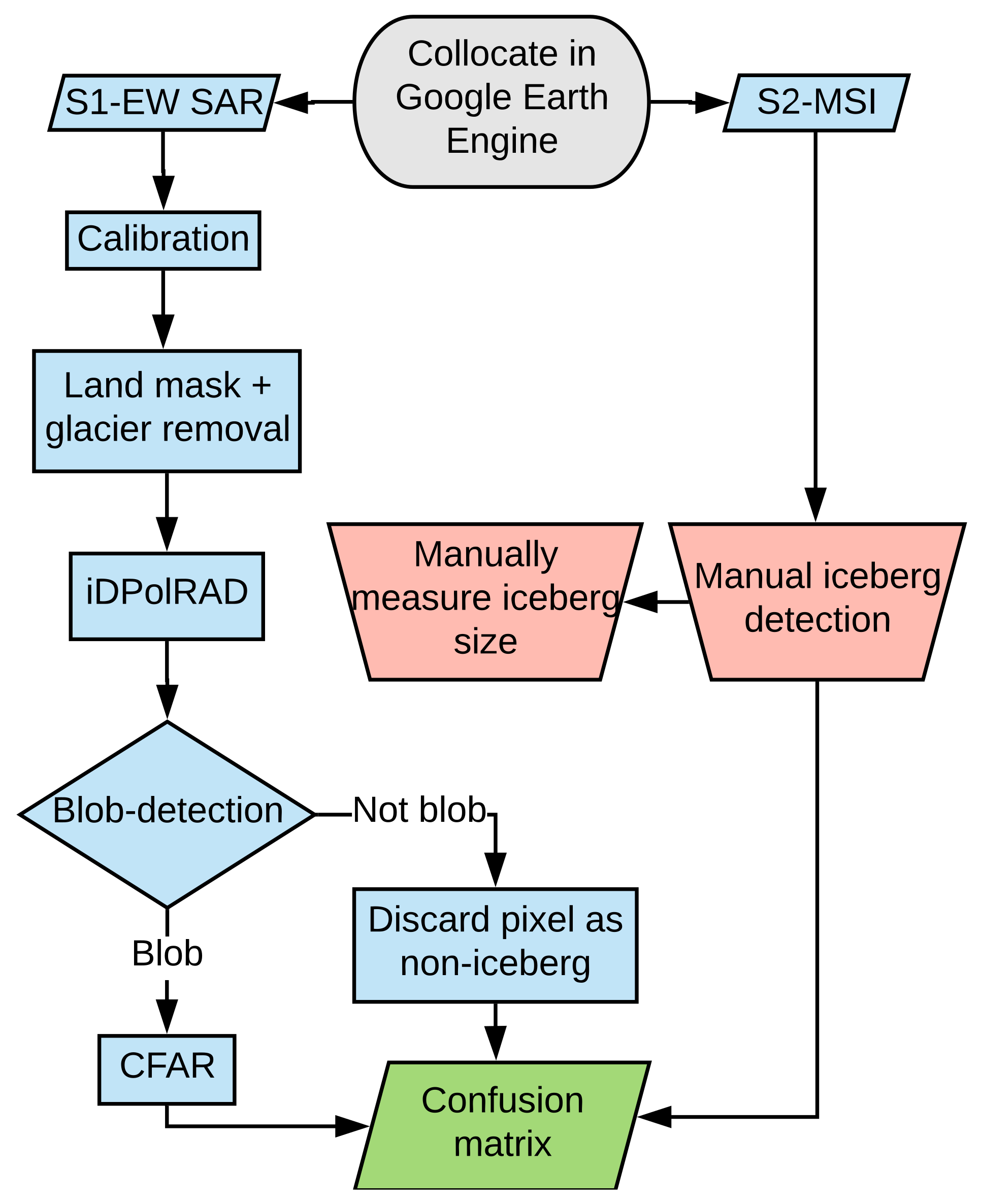
3.1. Overview
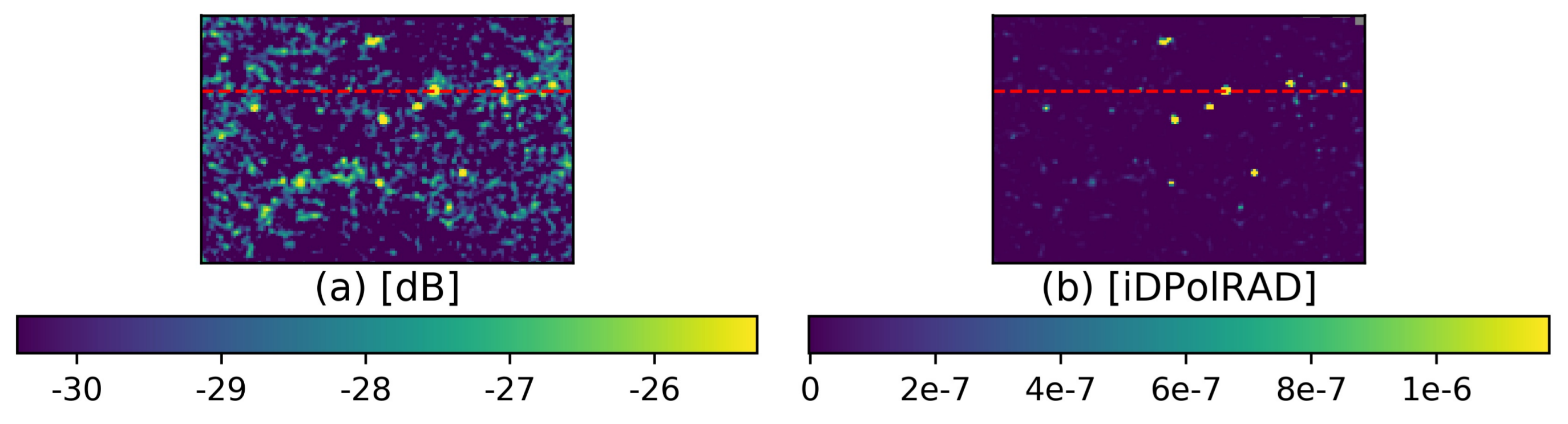
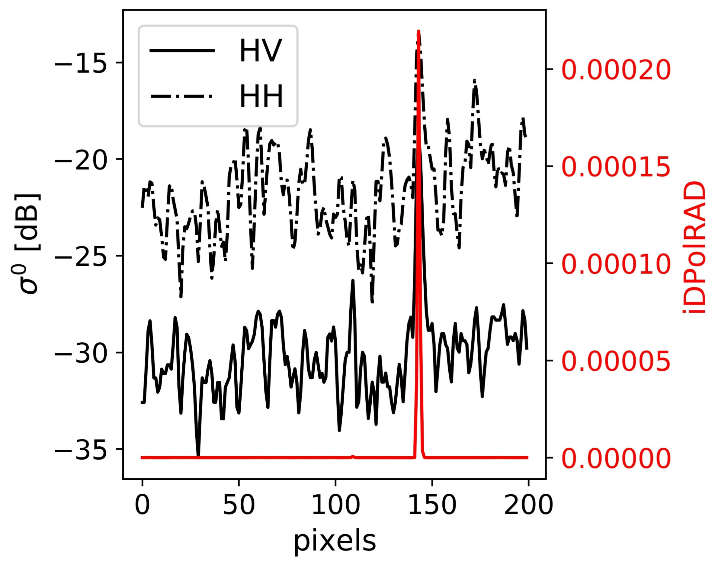
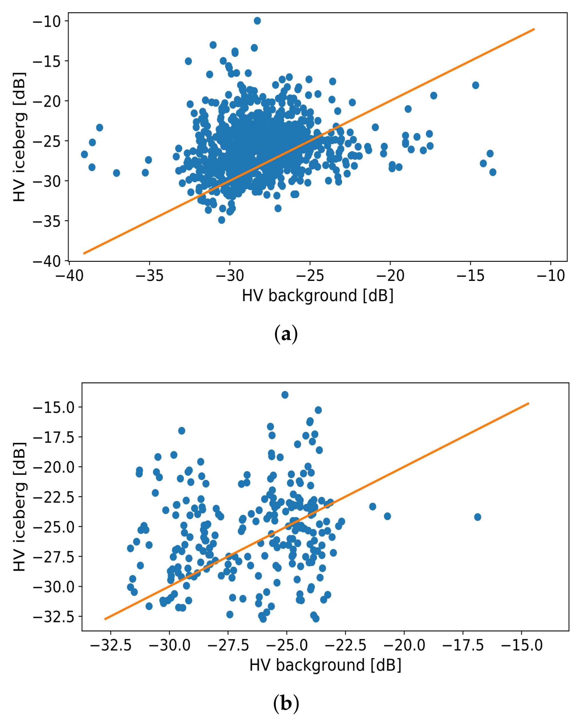
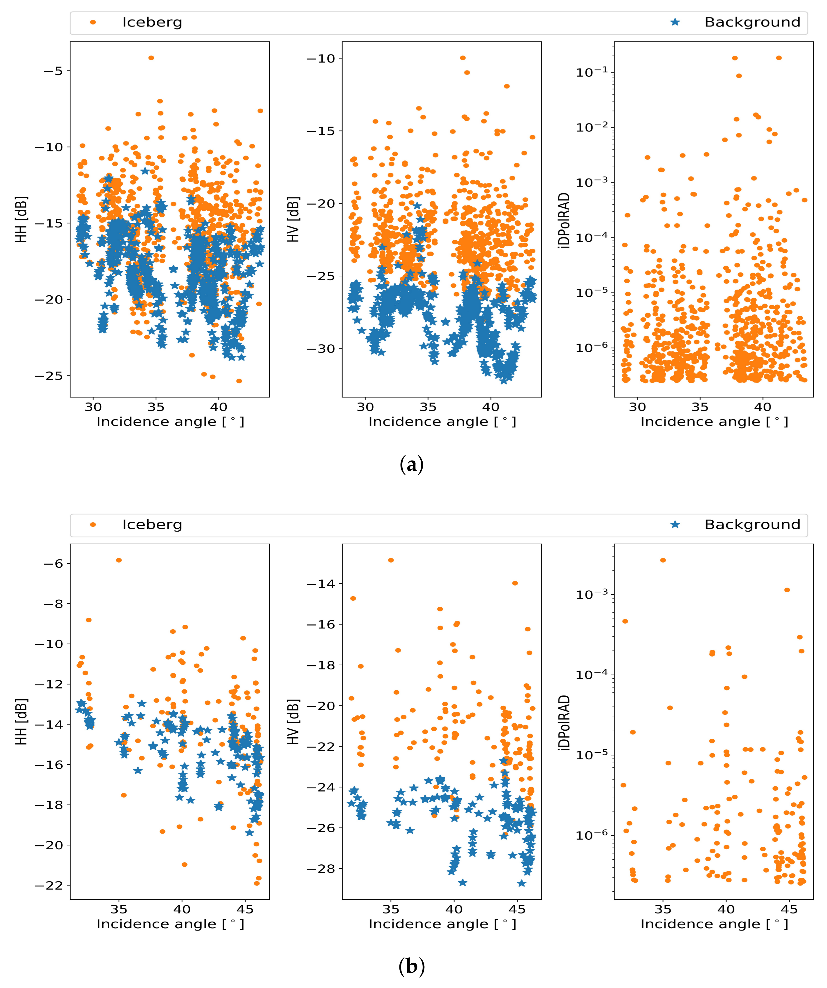
3.2. iDPolRAD
3.3. Blob-Detector
3.4. A Modified Constant False Alarm Rate Algorithm
3.4.1. The Modified CFAR Approach
3.4.2. Fitting of the Probability Density Functions
3.4.3. Quality and Robustness of Probability Density Functions
3.4.4. Determination of Thresholds for the Modified CFAR
4. Results
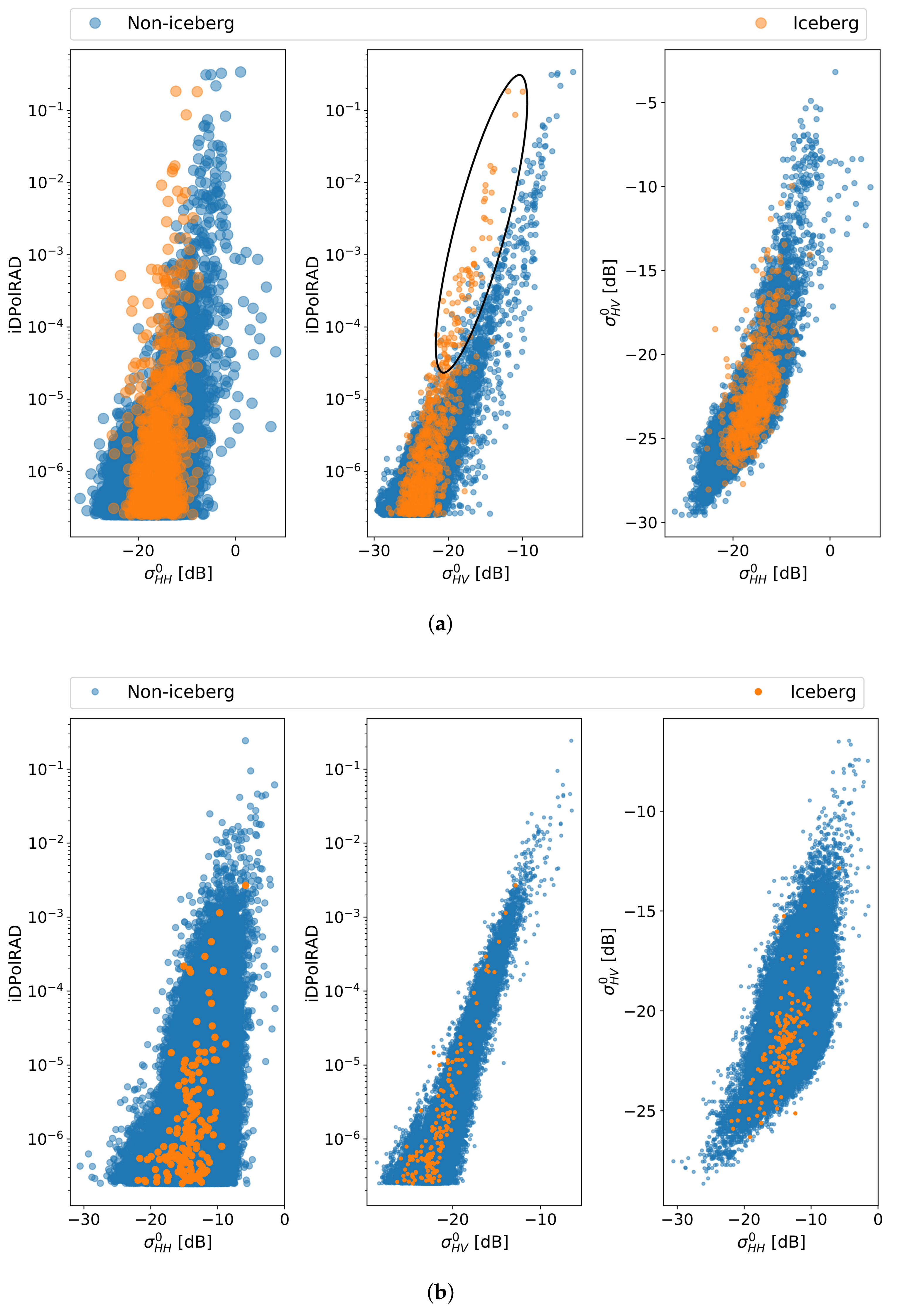
4.1. Detection Performance of the iDPolRAD-Filter
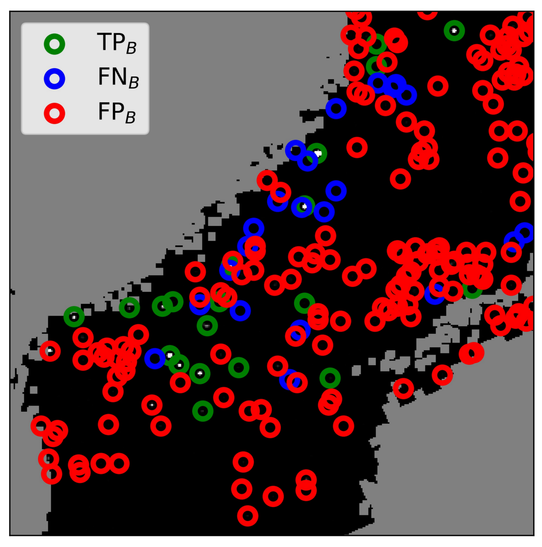
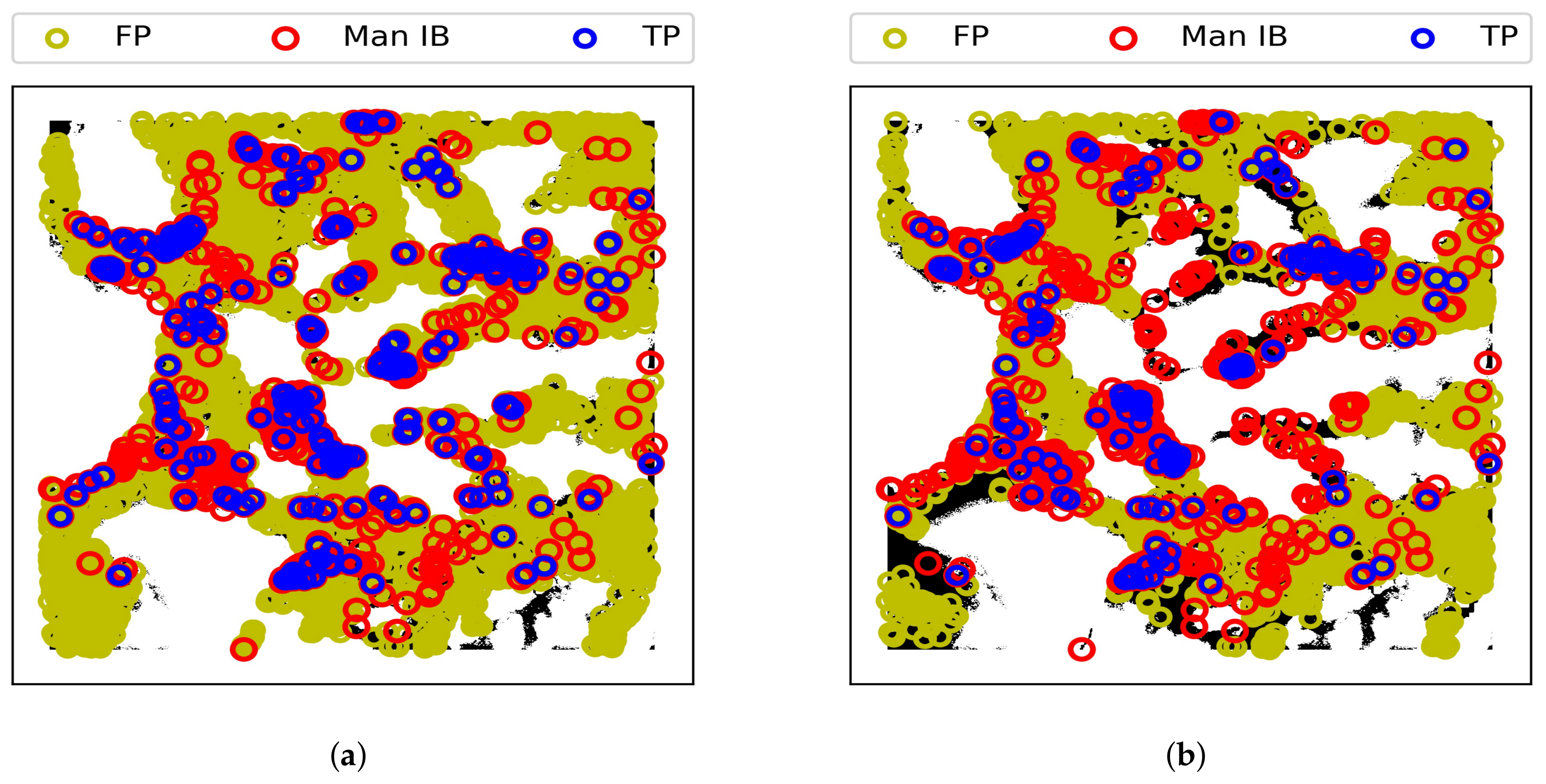
4.2. Blob Detection Results
4.3. PDF Fitting
4.3.1. Choosing
4.3.2. Representability and Quality of PDFs
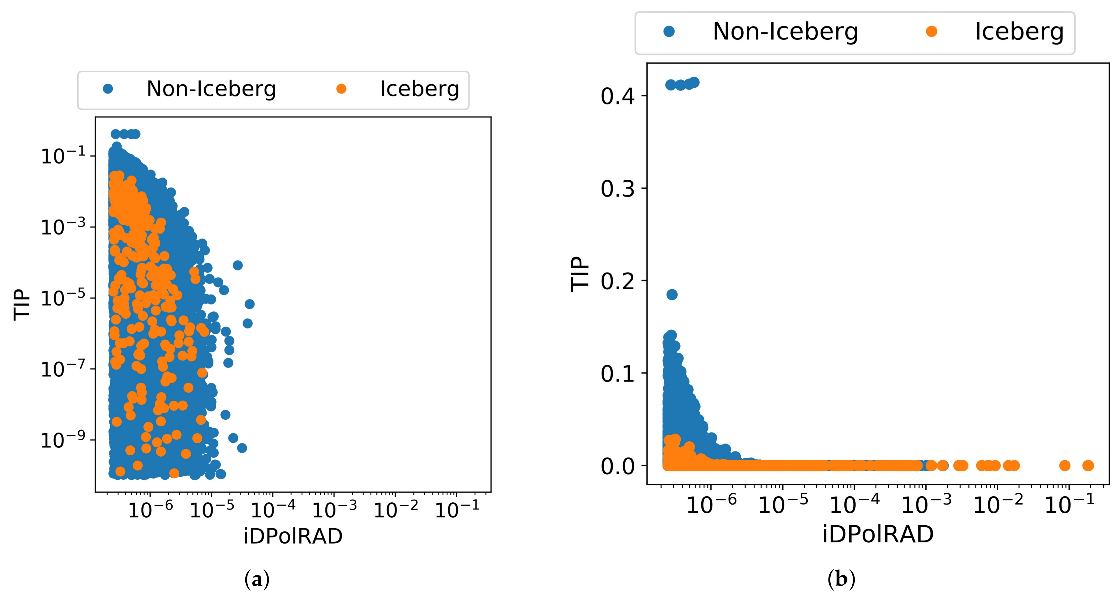
4.3.3. TIP
4.4. Confusion Matrix
4.5. Comparing Detection Results with and without Blob Detection
4.6. Testing Algorithm for Different Resolutions
5. Discussion
6. Conclusions
7. Data Availability
Author Contributions
Funding
Acknowledgments
Conflicts of Interest
Abbreviations
| CFAR | Constant False Alarm Rate |
| FJL | Franz Josef Land |
| ENL | Equivalent Number of Looks |
| EWS | Extra Wide Swath |
| GEE | Google Earth Engine |
| GEV | Generalized Extreme Value |
| iDPolRAD | intensity Dual-Polarization Ratio Anomaly Detector |
| IWS | Interferometric Wide Swath |
| MSI | Multi Spectral Imager |
| NA | Nord-Austlandet |
| NESZ | Noise Equivalent Sigma Zero |
| Probability Density Function | |
| PFA | Probability of False Alarm |
| SAR | Synthetic Aperture Radar |
| TIP | Tail Integrated Probability |
References
- Jackson, C.R.; Apel, J.R. Synthetic Aperture Radar: Marine User’s Manual; US Department of Commerce, National Oceanic and Atmospheric Administration, National Environmental Satellite, Data, and Information Service (NESDIS), Office of Research and Applications: Washington, DC, USA, 2004; p. 411. [Google Scholar]
- Wesche, C.; Dierking, W. Iceberg signatures and detection in SAR images in two test regions of the Weddell Sea, Antarctica. J. Glaciol. 2012, 58, 325–339. [Google Scholar] [CrossRef]
- Silva, T.A.; Bigg, G.R. Computer-based identification and tracking of Antarctic icebergs in SAR images. Remote Sens. Environ. 2005, 94, 287–297. [Google Scholar] [CrossRef]
- Power, D.; Youden, J.; Lane, K.; Randell, C.; Flett, D. Iceberg detection capabilities of RADARSAT synthetic aperture radar. Can. J. Remote Sens. 2001, 27, 476–486. [Google Scholar] [CrossRef]
- Williams, R.; Rees, W.; Young, N. A technique for the identification and analysis of icebergs in synthetic aperture radar images of Antarctica. Int. J. Remote Sens. 1999, 20, 3183–3199. [Google Scholar] [CrossRef]
- Willis, C.; Macklin, J.; Partington, K.; Teleki, K.; Rees, W.; Williams, R. Iceberg detection using ERS-1 synthetic aperture radar. Int. J. Remote Sens. 1996, 17, 1777–1795. [Google Scholar] [CrossRef]
- Norwegian Petroleum Directorate. NPD FactMaps Standard. Available online: http://gis.npd.no/Factmaps/html_21/ (accessed on 6 August 2018).
- Arctic Council. Arctic Marine Shipping Assessment 2009 Report; Arctic Council: Tromsø, Norway, 2009. [Google Scholar]
- Keghouche, I.; Counillon, F.; Bertino, L. Modeling dynamics and thermodynamics of icebergs in the Barents Sea from 1987 to 2005. J. Geophys. Res. Ocean. 2010, 115. [Google Scholar] [CrossRef]
- Sandven, S.; Babiker, M.; Kloster, K. Iceberg observations in the Barents Sea by radar and optical satellite images. In Proceedings of the ENVISAT Symposium, Montreux, Switzerland, 23–27 April 2007. [Google Scholar]
- National Snow and Ice Data Center. Cryosphere Glossary: Fast Ice. Available online: https://nsidc.org/cryosphere/glossary/term/fast-ice (accessed on 24 July 2018).
- Marino, A.; Dierking, W.; Wesche, C. A Depolarization Ratio Anomaly Detector to identify icebergs in sea ice using dual-polarization SAR images. IEEE Trans. Geosci. Remote Sens. 2016, 54, 5602–5615. [Google Scholar] [CrossRef]
- Gill, R.S. Operational Detection of Sea Ice Edges and Icebergs Using SAR. Can. J. Remote Sens. 2001, 27, 411–432. [Google Scholar] [CrossRef]
- Frost, A.; Ressel, R.; Lehner, S. Automated Iceberg Detection Using High-Resolution X-Band SAR Images. Can. J. Remote Sens. 2016, 42, 354–366. [Google Scholar] [CrossRef]
- Collecte Localisation Satellites (CLS). Sentinel-1 Product Definition; Report 2.7; European Space Agency: Frascati, Italy, 2016. [Google Scholar]
- European Space Agency. User Guide—Sentinel SAR—Level-1 Ground Range Detected. Available online: https://sentinel.esa.int/web/sentinel/user-guides/sentinel-1-sar/resolutions/level-1-ground-range-detected (accessed on 11 October 2018).
- Korosov, A.; Hansen, M.; Dagestad, K.F.; Yamakawa, A.; Vines, A.; Riechert, M. Nansat: A scientist-orientated python package for geospatial data processing. J. Open Res. Softw. 2016, 4. [Google Scholar] [CrossRef]
- Miranda, N.; Meadows, P. Radiometric Calibration of S-1 Level-1 Products Generated by the S-1 IPF. 2015. Available online: https://Sentinel.Esa.Int/Doc./247904/685163/S1-Radiom.-Calibration-V1.0.Pdf (accessed on 10 October 2018).
- Carroll, M.L.; Townshend, J.R.; DiMiceli, C.M.; Noojipady, P.; Sohlberg, R.A. A new global raster water mask at 250 m resolution. Int. J. Digit. Earth 2009, 2, 291–308. [Google Scholar] [CrossRef]
- Korosov, A.A.; Rampal, P. A combination of feature tracking and pattern matching with optimal parametrization for sea ice drift retrieval from SAR data. Remote Sens. 2017, 9, 258. [Google Scholar] [CrossRef]
- Gorelick, N.; Hancher, M.; Dixon, M.; Ilyushchenko, S.; Thau, D.; Moore, R. Google Earth Engine: Planetary-scale geospatial analysis for everyone. Remote Sens. Environ. 2017. [Google Scholar] [CrossRef]
- Nunziata, F.; Migliaccio, M.; Brown, C.E. Reflection symmetry for polarimetric observation of man-made metallic targets at sea. IEEE J. Ocean. Eng. 2012, 37, 384–394. [Google Scholar] [CrossRef]
- Marino, A. A notch filter for ship detection with polarimetric SAR data. IEEE J. Sel. Top. Appl. Earth Obs. Remote Sens. 2013, 6, 1219–1232. [Google Scholar] [CrossRef]
- Dierking, W.; Wesche, C. C-Band Radar Polarimetry—Useful for Detection of Icebergs in Sea Ice. IEEE Trans. Geosci. Remote Sens. 2014, 52, 25–37. [Google Scholar] [CrossRef]
- Scikit-Image. Blob Detection. Available online: http://scikit-image.org/docs/dev/auto_examples/features_detection/plot_blob.html (accessed on 24 July 2018).
- Lindeberg, T. Feature detection with automatic scale selection. Int. J. Comput. Vis. 1998, 30, 79–116. [Google Scholar] [CrossRef]
- SciPy. Statistical Functions. Available online: https://docs.scipy.org/doc/scipy/reference/stats.html (accessed on 25 July 2018).
- Engineering Statistics Handbook. Kolmogorov–Smirnoc Goodness-of-Fit Test. Available online: https://www.itl.nist.gov/div898/handbook/eda/section3/eda35g.htm (accessed on 25 July 2018).
- Dierking, W. Mapping of Different Sea Ice Regimes Using Images From Sentinel-1 and ALOS Synthetic Aperture Radar. IEEE Trans. Geosci. Remote Sens. 2010, 48, 1045–1058. [Google Scholar] [CrossRef]
- Dierking, W. Technical Assistance for the Deployment of Airborne SAR and Geophysical Measurements during the ICESAR 2007; Final Report—Part 2: Sea Ice; ESA-ESTEC: Noordwijk, The Netherlands, 2008. [Google Scholar]


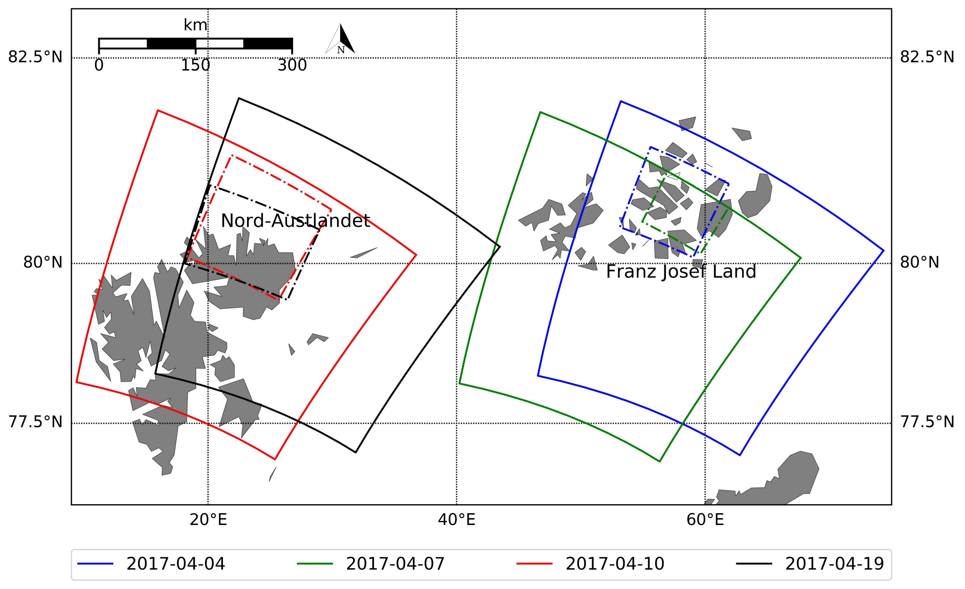
| Date (Year-Month-Day), Time | Region | S1-File | Part of Image [No of Rows, No of Columns] | Incidence Angle Range [] |
|---|---|---|---|---|
| 2017-04-04 03:38:14 | FJL | S1A_EW_GRDM_1SDH_20170404T033814_ 20170404T033918_015989_01A5F5_FB23 | 3000 × 3000 | 36–43 |
| 2017-04-07 04:02:57 | FJL | S1A_EW_GRDM_1SDH_20170407T040257_ 20170407T040402_016033_01A74D_1347 | 2500 × 2000 | 28–35 |
| 2017-04-10 06:06:23 | NA | S1A_EW_GRDM_1SDH_20170410T060623_ 20170410T060727_016078_01A8B3_8486 | 4000 × 4000 | 30–40 |
| 2017-04-19 05:41:40 | NA | S1A_EW_GRDM_1SDH_20170419T054140_ 20170419T054244_016209_01ACB5_82A4 | 3000 × 4300 | 36–46 |
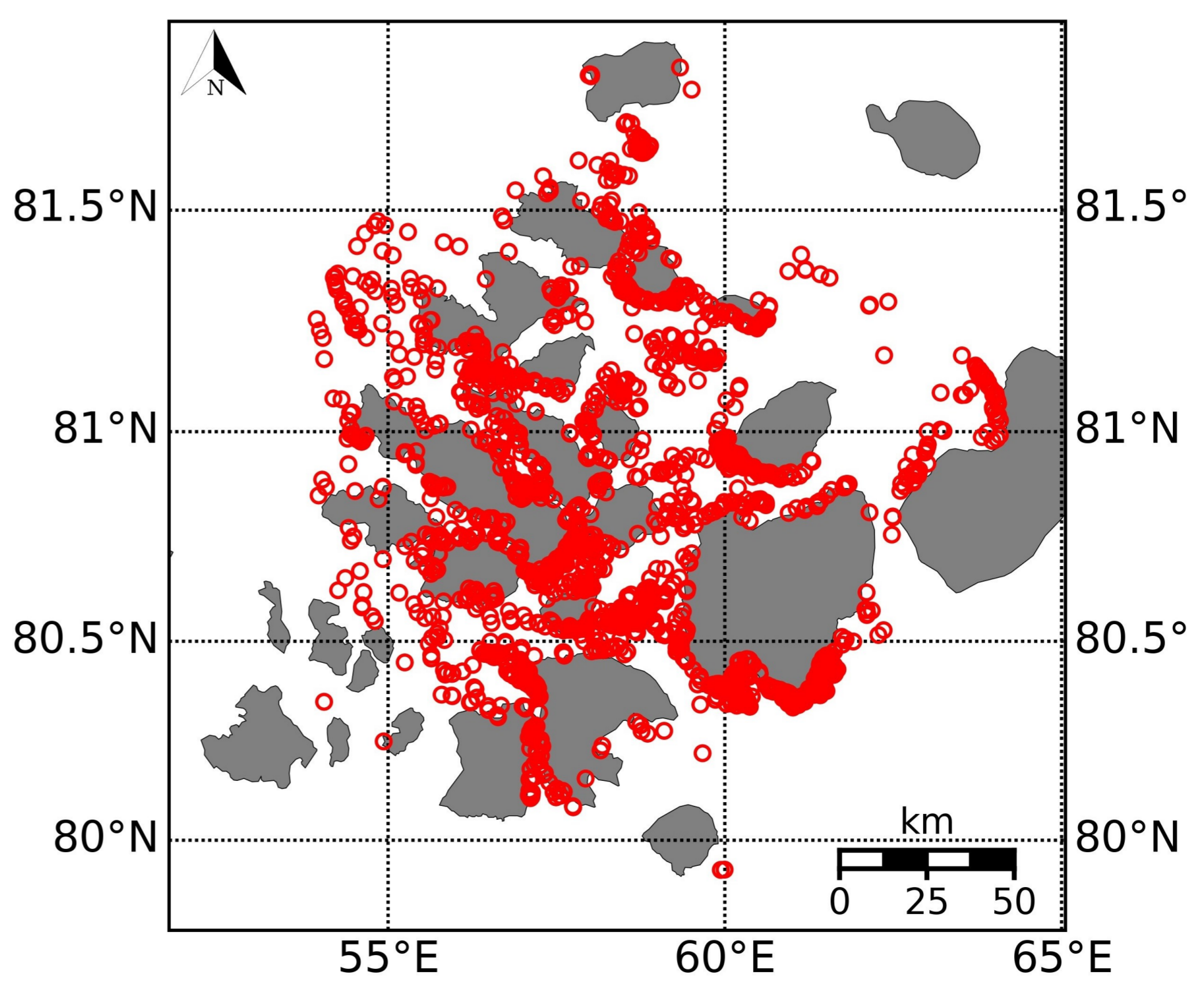
| Date (Year-Month-Day), Time | Region | Ice Type [Fast Ice] | Number of Manually Detected Icebergs | T 12:00 UTC [C] |
|---|---|---|---|---|
| 2017-04-04 11:46:41 | FJL | Smooth | 2292 | −20.7 |
| 2017-04-07 11:56:40 | FJL | Smooth | 2940 | −19.9 |
| 2017-04-10 13:47:25 | NA | Rough | 688 | −9.7 |
| 2017-04-19 14:17:39 | NA | Rough | 827 | −12.5 |
| Name | Description |
|---|---|
| True Positives () | Pixels that are selected by automatic blob detection and are manually defined as icebergs |
| False Positives () | Pixels that are selected by automatic blob detection but are not manually defined as icebergs |
| False Negatives () | Pixels that are not selected by automatic blob detection but are manually defined as icebergs |
| True Negatives () | Pixels that are not selected by automatic blob detection and are not manually defined as icebergs |
| Equation | Parameters | |
|---|---|---|
| Gamma | a = shape parameter = inverse scale parameter | |
| Generalized Gamma | a, c = shape parameter | |
| Generalized Extreme Value | , if c = 0 | c = shape parameter |
| Total = | Actual Iceberg | Actual Non-Iceberg |
|---|---|---|
| Predicted iceberg | ||
| Predicted non-iceberg |
| ( = 0.1) | Time [s] | |||
|---|---|---|---|---|
| 321 | 489 | 14,492 | 533 | |
| 413 | 400 | 28,090 | 2172 | |
| 677 | 187 | 81,390 | 18,498 |
| () | Time [s] | |||
|---|---|---|---|---|
| 0.1 (1 layer) | 413 | 400 | 28,090 | 2172 |
| 0.5 (1 layer) | 305 | 500 | 13,317 | 502 |
| 2–3 (2 layers) | 135 | 670 | 1505 | 12 |
| Image Data Date (Year-Month-Day) Time | Part of Image [No of Rows, No of Columns] | Time [s] | |||
|---|---|---|---|---|---|
| 2017-04-04 11:46:41 | 413 | 400 | 28,090 | 3000 × 3000 | 2172 |
| 2017-04-07 11:56:40 | 370 | 310 | 14,307 | 2500 × 2000 | 563 |
| 2017-04-10 13:47:25 | 65 | 47 | 148,299 | 4000 × 4000 | 54,880 |
| 2017-04-19 14:17:39 | 94 | 86 | 99,282 | 3000 × 4300 | 26,322 |
| Gamma | Generalized Gamma | GEV | |
|---|---|---|---|
| 61 × 61 | 0.21 ± 0.08 | 0.19 ± 0.06 | 0.19 ± 0.08 |
| 101 × 101 | 0.19 ± 0.08 | 0.16 ± 0.06 | 0.18 ± 0.07 |
| 141 × 141 | 0.19 ± 0.12 | 0.15 ± 0.07 | 0.17 ± 0.09 |
| Gamma [%] | Generalized Gamma [%] | GEV [%] | |
|---|---|---|---|
| Full image | 0.28 | 0.17 | 0.19 |
| Sub-images | 0.19 ± 0.12 | 0.15 ± 0.07 | 0.17 ± 0.09 |
| PFA | ||||
|---|---|---|---|---|
| 2017-04-04 | ||||
| 237 | 176 | 10,182 | 17,908 | |
| 178 | 235 | 2890 | 25,200 | |
| 151 | 262 | 1273 | 26,817 | |
| 2017-04-07 | ||||
| 184 | 186 | 4565 | 9742 | |
| 121 | 249 | 1685 | 12,622 | |
| 88 | 282 | 906 | 13401 | |
| 2017-04-10 | ||||
| 21 | 44 | 44,007 | 4292 | |
| 11 | 54 | 15,679 | 132,620 | |
| 10 | 55 | 7941 | 140,358 | |
| 2017-04-19 | ||||
| 34 | 60 | 26,445 | 72,837 | |
| 15 | 79 | 8590 | 90,692 | |
| 8 | 86 | 4240 | 95,042 |
| Date (Year-Month-Day) | [%] | [%] | [%] |
|---|---|---|---|
| 2017-04-04 | 94.2 | 21.9 | 78.1 |
| 2017-04-07 | 93.3 | 17.8 | 82.2 |
| 2017-04-10 | 99.9 | 9.7 | 90.3 |
| 2017-04-19 | 99.8 | 8.3 | 91.7 |
| Acquisition Mode | |||
|---|---|---|---|
| Sentinel-1 EWS | 29 | 39 | 221 |
| Sentinel-1 IWS | 34 | 51 | 426 |
| Acquisition Mode | [%] | [%] | [%] |
|---|---|---|---|
| Sentinel-1 EWS | 41.6 | 20.6 | 79.4 |
| Sentinel-1 IWS | 87.5 | 38.8 | 61.2 |
© 2019 by the authors. Licensee MDPI, Basel, Switzerland. This article is an open access article distributed under the terms and conditions of the Creative Commons Attribution (CC BY) license (http://creativecommons.org/licenses/by/4.0/).
Share and Cite
Soldal, I.H.; Dierking, W.; Korosov, A.; Marino, A. Automatic Detection of Small Icebergs in Fast Ice Using Satellite Wide-Swath SAR Images. Remote Sens. 2019, 11, 806. https://doi.org/10.3390/rs11070806
Soldal IH, Dierking W, Korosov A, Marino A. Automatic Detection of Small Icebergs in Fast Ice Using Satellite Wide-Swath SAR Images. Remote Sensing. 2019; 11(7):806. https://doi.org/10.3390/rs11070806
Chicago/Turabian StyleSoldal, Ingri Halland, Wolfgang Dierking, Anton Korosov, and Armando Marino. 2019. "Automatic Detection of Small Icebergs in Fast Ice Using Satellite Wide-Swath SAR Images" Remote Sensing 11, no. 7: 806. https://doi.org/10.3390/rs11070806
APA StyleSoldal, I. H., Dierking, W., Korosov, A., & Marino, A. (2019). Automatic Detection of Small Icebergs in Fast Ice Using Satellite Wide-Swath SAR Images. Remote Sensing, 11(7), 806. https://doi.org/10.3390/rs11070806